Cosmic-ray driven dynamo
in the interstellar medium of irregular galaxies

Abstract

Context. Irregular galaxies are usually smaller and less massive than their spiral, S0, and elliptical counterparts. Radio observations indicate that a magnetic field is present in irregular galaxies whose value is similar to that in spiral galaxies. However, the conditions in the interstellar medium of an irregular galaxy are unfavorable for amplification of the magnetic field because of the slow rotation and low shearing rate.

Aims. We investigate the cosmic-ray driven dynamo in the interstellar medium of an irregular galaxy. We study its efficiency under the conditions of slow rotation and weak shear. The star formation is also taken into account in our model and is parametrized by the frequency of explosions and modulations of activity.

Methods. The numerical model includes a magnetohydrodynamical dynamo driven by cosmic rays that is injected into the interstellar medium by randomly exploding supernovae. In the model, we also include essential elements such as vertical gravity of the disk, differential rotation approximated by the shearing box, and resistivity leading to magnetic reconnection.

Results. We find that even slow galactic rotation with a low shearing rate amplifies the magnetic field, and that rapid rotation with a low value of the shear enhances the efficiency of the dynamo. Our simulations have shown that a high amount of magnetic energy leaves the simulation box becoming an efficient source of intergalactic magnetic fields.

1 Introduction

Irregular galaxies have lower masses than typical spirals and ellipticals. In addition, they have irregular distributions of the star-forming regions, and rotations that are slower than spiral galaxies by half an order of magnitude (Gallagher & Hunter 1984). The rotation curves of irregular galaxies are non-uniform and have a weak shear.

Radio observations of magnetic fields in spiral galaxies indicate that their magnetic fields have strong ordered (1–5 $\mu$G) and random (9–15 $\mu$G) components (Beck 2005). A plausible process fueling the growth in the magnetic energy and flux of these galaxies is magnetohydrodynamical dynamo (Widrow 2002; Gressel et al. 2008). The vital conditions required for the dynamo to effectively amplify the magnetic field are rapid rotation and shear. In irregular galaxies, both quantities seem to be too low to initiate efficient dynamo action. In contrast, the observations of magnetic field in irregular galaxies indicate that these galaxies could have strong and ordered magnetic fields (e.g., Chyży et al. 2000, 2003; Kepley et al. 2007; Lisenfeld et al. 2004).

The most spectacular radio observations to date of irregulars were those performed for the galaxy NGC 4449 (Chyży et al. 2000). The total strength of its magnetic field is about $14\leavevmode\nobreak\ \mu$G with a ordered component reaching locally values of $8\leavevmode\nobreak\ \mu$G. These are similar to the intensities observed for large spirals. A high number of H ii regions and slow rotation is also observed with quite large velocity shear (Valdez-Gutiérrez et al. 2002). The radio observations of H i around the galaxy indicate that this object is embedded in two large H i systems that counter-rotate with respect to the optical part of this galaxy (Bajaja et al. 1994; Hunter et al. 1998, 1999). In addition to these H i clouds, NGC 4449 contains an unusual ring of H i in the outer part of the optical disk (Hunter et al. 1999). This complicated topology of the H i velocity field could help in achieving efficient magnetic field amplification (see Otmianowska-Mazur et al. 2000).

Chyży et al. (2003) found that two other irregular galaxies, NGC 6822 and IC 10 are also magnetized. The former has a very low total magnetic field weaker than 5 $\mu$G, a small number of H ii regions, and almost rigid rotation (see Sect. 2). These properties are directly related to the efficiency of the dynamo process in galaxies (see Otmianowska-Mazur et al. 2000; Hanasz et al. (2006, 2009) that weakly amplifies the magnetic field in this galaxy. The irregular IC 10 has a total magnetic field strength that varies between 5 and 15 $\mu$G with no ordered component. Observations performed by Chyży et al. (2003) indicate that the total magnetic field is correlated with the number of H ii regions. The number of the regions is higher than in NGC 6822, and the rotation of IC 10 has a partly differential character (see Sect. 2). Both conditions lead to more rapid magnetic field amplification than for NGC 6822. As for NGC 4449, IC 10 is embedded in a large cloud of H i, which counter-rotates with respect to the inner disk (Wilcots & Miller 1998).

Klein et al. (1993) inferred that the Large Magellanic Cloud (LMC) has a large-scale magnetic field that has the shape of a trailing spiral structure, similar to normal spiral galaxies. It is possible that the amplification of the magnetic field is connected to the differential rotation of this galaxy present beyond a certain radius (Klein et al. 1993; Luks & Rohlfs 1992; Gaensler et al. 2005).

We note that polarized radio emission is detected in the irregular galaxy NGC 1569. This galaxy has a very high star formation rate (Martin 1998) and exhibits bursts of activity in its past (Vallenari & Bomans 1996). The radio observation of this galaxy by Lisenfeld et al. (2004) found that the galaxy has large-scale magnetic fields in the disk and halo. Furthermore, they found that their data agree that a convective wind could allow for escape of cosmic-ray electrons in to the halo. These observations are the main reason for undertaking our CR-driven dynamo calculations in irregular galaxies. In addition to Lisenfeld et al. (2004), the radio observations of Kepley et al. (2007) showed that the large-scale magnetic arms visible in NGC 1569 are aligned perpendicularly to the disk and that the northern part of the disk of the galaxy is inclined at a different angle.

Kronberg et al. (1999) realized that dwarf galaxies (apart from their low masses) could serve as an efficient source of gas and magnetic fields in the intergalactic medium (IGM) during their initial bursts of star formation in the early Universe. In the case of star-forming dwarf galaxies, we expect that the dominant driver of a galactic wind are cosmic rays, in contrast to large spirals, such as the Milky Way, where the thermal driving is most significant (Everett et al. 2008). Therefore, we applied the model of the CR-driven dynamo to the interstellar medium and conditions of an irregular galaxy and try to find how much of the magnetic energy can be expelled from the dwarf galaxies to the IGM.

Many questions about magnetic field amplification in irregular galaxies remain unresolved. The physical explanation of this process is difficult to establish because these galaxies rotate slowly, almost like a solid body. In this paper, we check how our model of cosmic-ray driven dynamo, which effectively describes spiral galaxies (Hanasz et al. 2004, 2006, 2009), can be applied to irregular galaxies. In the present numerical experiment we attempt to answer how the model input parameters observed in irregulars (small gravitational potential, gas density, low rotation, and small shear) influence the magnetic fields within them. We have not taken into account the magnetic field possibly injected by stars. We plan to study this in the future. We found that in certain conditions achievable for irregulars it is possible to have efficient magnetic field amplification.

2 Observations of irregular galaxies

Table 1: Main properties of NGC 4449, NGC 6822, and IC 10

	NGC 4449	NGC 6822	IC 10
Type	IBm	IB(s)m	dIrr
Distance [Mpc]	4.21	0.50	0.66
Diameter [kpc]	5.73	1.71	1.27
SFR	high	low	high
$<\!B_{\textrm{tot}}\!>$ [$\mu$G]	5–15	$\leq 5$	5–15
$<\!B_{\textrm{reg}}\!>$ [$\mu$G]	$\simeq 8$	$\leq 3$	$\leq 3$

In the following rows we present: the morphological type of the object (LEDA), the distance (Karachentsev et al. 2004), the size calculated from $D_{25}$ (LEDA) and distance, the star formation rate (SFR), and the results of the radio analysis of Chyży et al. (2000, 2003).

To study properties of the irregulars and determine the input parameters for our simulations, we use observations of NGC 4449, NGC 6822, and IC 10 acquired by Chyży et al. (2000, 2003). The main properties of these objects are presented in Table 1.

From the rotation curves of IC 10 (Fig. 1, top panel, solid line) obtained by Wilcots & Miller 1998, NGC 6822 (Fig. 1, top panel, dashed line) obtained by Weldrake et al. 2003, and NGC 4449 (Fig. 1, top panel, dot-dashed line) by Valdez-Gutiérrez et al. 2002, we computed the angular velocity and shearing rate of each galaxy (see Sect. 5.1). For the two first galaxies, we use H i data. In the case of NGC 4449, we restricted our analysis to the internal region and used H$\alpha$ data, because of its very complex velocity pattern.

In the velocity pattern of the IC10, we can see a central part with a solid-body rotation, which flattens to a constant value $v_{\mathrm{rot}}\simeq 30$ km s^-1 at $r=352$ pc. The NGC 6822 rotation curve is a monotonically increasing function with a square root slope and the highest value $v_{\mathrm{rot}}\simeq 60$ km s^-1 at $r=5.7$ kpc. The rotation curve of NGC 4449 is highly disturbed and reaches a maximum value of $v_{\mathrm{rot}}\simeq 40$ km s^-1 at radius of 2 kpc.

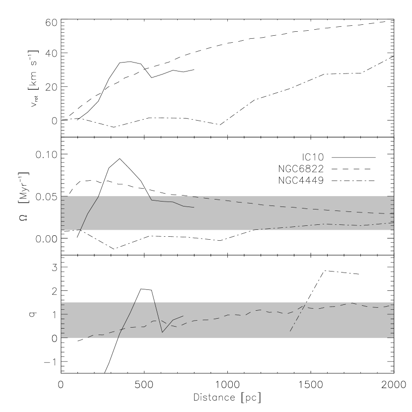
Figure 1: Observational rotation characteristics of IC 10, NGC 6822, and NGC 4449. We present, from top to bottom: the rotation curves (references in Sect. 2), the calculated angular velocity, and the computed shear parameter $q$ (for details see Sect. 5.1) respectively. The shaded region marks the range of parameters presented in this paper.

3 Description of the model

The CR-driven dynamo model consists of the following elements (based on Hanasz et al. 2004, 2006):

• The cosmic ray component is a relativistic gas described by a diffusion-advection transport equation. Typical values of the diffusion coefficient are $(3\div 5)\times 10^{28}\leavevmode\nobreak\ \textrm{cm}^{2}\leavevmode\nobreak\ \textrm{s}^{-1}$ (see Strong et al. 2007) at energies of around $1\leavevmode\nobreak\ \textrm{GeV}$, although in our simulations we use reduced values (see Sect. 4.1).

• Anisotropic diffusion of CR. Following Giacalone & Jokipii (1999) and Jokipii (1999), we assume that the CR gas diffuses anisotropically along magnetic field lines. The ratio of the perpendicular to parallel CR diffusion coefficients suggested by the authors is $5\%$.

• Localized sources of CR. In the model, we apply the random explosions of supernovae in the disk volume. Each explosion is a localized source of cosmic rays. The cosmic ray input of individual SN remnant is $10\%$ of the canonical kinetic energy output ($10^{51}\leavevmode\nobreak\ \textrm{erg}$) and distributed over several subsequent time steps.

• Resistivity of the ISM to enable the dissipation of the small-scale magnetic fields (see Hanasz et al. 2002 and Hanasz & Lesch 2003). In the model, we apply the uniform resistivity and neglect the Ohmic heating of gas by the resistive dissipation of magnetic fields.

• Shearing boundary conditions and tidal forces following the prescription by Hawley, Gammie & Balbus (1995), are implemented to reproduce the differentially rotating disk in the local approximation.

• Realistic vertical disk gravity following the model by Ferrière (1998) modified by reducing the contribution of disk and halo masses by one order of the magnitude, to adjust the irregular galaxy environment.

We apply the following set of resistive MHD equations:

$$\frac{\partial\rho}{\partial t} + \mathbf{\nabla}\cdot(\rho\mathbf{V})=0,$$ (1)

$$\frac{\partial e}{\partial t} + \mathbf{\nabla}\cdot(e\mathbf{V})=-p(\mathbf{\nabla}\cdot\mathbf{V}),$$ (2)

$$\frac{\partial\mathbf{V}}{\partial t} + (\mathbf{V}\cdot\mathbf{\nabla})\mathbf{V}=-\frac{1}{\rho}\mathbf{\nabla}\left(p+p_{\rm cr}+\frac{B^{2}}{8\pi}\right)$$ (3)

$$+ \frac{\mathbf{B}\cdot\mathbf{\nabla B}}{4\pi\rho}-2\mathbf{\Omega}\times\mathbf{V}+2q\Omega^{2}x\hat{\@vec{e}}_{x},$$

$$\frac{\partial\@vec{B}}{\partial t} = \mathbf{\nabla}\times(\@vec{V}\times\@vec{B})+\eta\mathbf{\triangle}\@vec{B},$$ (4)

$$p = (\gamma-1)e,\,\;\gamma=5/3,$$ (5)

where $q=-d\ln\Omega/d\ln R$ is the shearing rate, $R$ is a galactocentric radius, $\eta$ represents the ISM resistivity, $\gamma$ is the adiabatic index of thermal gas, $p_{\rm cr}$ is the cosmic-ray pressure, and the other symbols have their usual meaning. In the equation of motion, the term $\nabla p_{\rm cr}$ is included (see Berezinskii et al. 1990). The thermal gas is approximated by an adiabatic medium.

The cosmic ray component is an additional fluid described by the diffusion-advection equation (see e.g., Schlickeiser & Lerche 1985)

$$\frac{\partial e_{\rm cr}}{\partial t}+\mathbf{\nabla}(e_{\rm cr}\@vec{V})=\mathbf{\nabla}(\hat{K}\mathbf{\nabla}e_{\rm cr})-p_{\rm cr}(\mathbf{\nabla}\cdot\@vec{V})+Q_{\rm SN},$$ (6)

where $Q_{\rm SN}$ is the source term of the cosmic-ray energy density injected locally from randomly exploding SN remnants. The cosmic-ray fluid is described by an adiabatic equation of state with adiabatic index $\gamma_{\rm cr}$:

$$p_{\rm cr}=(\gamma_{\rm cr}-1)e_{\rm cr},\,\;\gamma_{\rm cr}=14/9.$$ (7)

The $\hat{K}$ is an diffusion tensor described by the formula:

$$K_{ij}=K_{\perp}\delta_{ij}+(K_{\parallel}-K_{\perp})n_{i}n_{j},\,\;n_{i}=B_{i}/B,$$ (8)

adopted following the argumentation of Ryu et al. (2003).

The vertical gravitational acceleration is taken from Ferrière (1998). We reduced both contributions of disk and halo by a factor of 10, the scale length of the exponential disk to $L_{D}=2$ kpc, and scale length of halo to $L_{H}=1$ kpc. In our computations, we incorporated the formula :

$$-g_{z}(R,Z)=(1.7\cdot 10^{-10}\;\textrm{cm s}^{-2})\frac{R_{*}^{2}+L_{H}^{2}}{R+L_{H}^{2}}\left(\frac{Z}{1\;\textrm{kpc}}\right)$$ (9)

$$+ (4.4\cdot 10^{-10}\;\textrm{cm s}^{-2})\exp\left(-\frac{R-R_{*}}{L_{D}}\right)\frac{Z}{\sqrt{Z^{2}+(0.2\;\textrm{kpc})^{2}}},$$

where $R_{*}$ is the distance of the origin of the simulation box from the galactic center and $Z$ is the height above the galactic mid plane.

4 Model setup and parameters

4.1 Model setup

The 3D cartesian domain size is $0.5\leavevmode\nobreak\ \textrm{kpc}\times 1\leavevmode\nobreak\ \textrm{kpc}\times 8\leavevmode\nobreak\ \textrm{kpc}$ in $x,y,z$ coordinates corresponding to the radial, azimuthal, and vertical directions, respectively. The grid size is $20\leavevmode\nobreak\ \textrm{pc}$ in each direction. The boundary conditions are sheared-periodic in $x$, periodic in $y$, and an outflow in $z$ direction. The domain is placed at the galactocentric radius $R_{*}=2$ kpc. In Fig. 2, we present example slices through the simulation domain. The left panel shows the CR energy density with the magnetic field vectors and the right panel shows the gas density with velocity vectors.

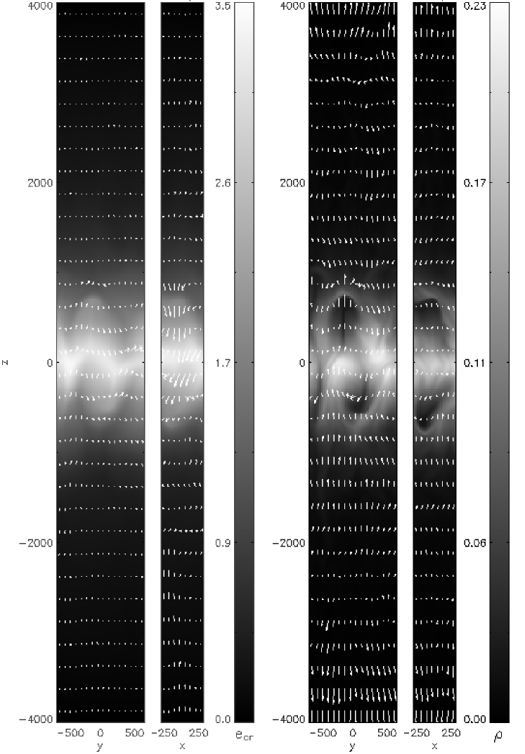
Figure 2: Example slices of a domain taken from simulation R.01Q1 at $t=660\leavevmode\nobreak\ \textrm{Myr}$. On the slices, the Parker loop is produced by cosmic rays from supernovae explosions.

The positions of SNe are chosen randomly with a uniform distribution in the $xy$ plane and a Gaussian distribution in the vertical direction. The scaleheight of SN explosions in the vertical direction is $100\leavevmode\nobreak\ \textrm{pc}$, and the CR energy that originates in an explosion is injected instantaneously into the ISM with a Gaussian radial profile ($r_{\it SN}=50\leavevmode\nobreak\ \textrm{pc}$). In addition, the SNe activity is modulated during the simulation time by a period $T_{p}$ and an activity time $T_{a}$.

The applied value of the perpendicular CR diffusion coefficient is $K_{\perp}=10^{3}\leavevmode\nobreak\ \textrm{pc}^{2}\leavevmode\nobreak\ \textrm{Myr}^{-1}=3\times 10^{26}\leavevmode\nobreak\ \textrm{cm}^{2}\leavevmode\nobreak\ \textrm{s}^{-1}$ and the parallel one is $K_{\parallel}=10^{4}\leavevmode\nobreak\ \textrm{pc}^{2}\leavevmode\nobreak\ \textrm{Myr}^{-1}=3\times 10^{27}\leavevmode\nobreak\ \textrm{cm}^{2}\leavevmode\nobreak\ \textrm{s}^{-1}$. The diffusion coefficients are $10\%$ of realistic values because of the simulation timestep, which becomes prohibitively short when the diffusion is too high.

The initial state of the system represents the magnetohydrostatic equilibrium with the horizontal, purely azimuthal magnetic field with $p_{\it mag}/p_{\it gas}=10^{-4}$, which corresponds to the mean value of magnetic field in the simulation box of 5 nG. Magnetic diffusivity $\eta$ is set to be 100 pc² Myr^-1, which corresponds to $3\times 10^{25}$ cm² s^-1 in cgs units (Lesch 1993). The column density of gas is $\varrho_{\it gas}=6\times 10^{20}\leavevmode\nobreak\ \textrm{cm}^{-2}$ (taken from observations, see Gallagher & Hunter 1984) and the initial value of the isothermal sound speed is set to be $c_{\it iso}=7\leavevmode\nobreak\ \textrm{km}\,\textrm{s}^{-1}$.

4.2 Model parameters

Table 2: List of models

Model	$\Omega$	$q$	$f$	$T_{p}$	$T_{a}$
	[Myr-1]		[kpc-2 Myr-1]	[Myr]	[Myr]
R.01Q1a	0.01	1	10	200	20
R.02Q1	0.02	1	10	200	20
R.03Q1b	0.03	1	10	200	20
R.04Q1	0.04	1	10	200	20
R.05Q1c	0.05	1	10	200	20
R.01Q0	0.01	0	10	200	20
R.01Q.5	0.01	0.5	10	200	20
R.01Q1a	0.01	1	10	200	20
R.01R1.5	0.01	1.5	10	200	20
R.05Q0	0.05	0	10	200	20
R.05Q.5	0.05	0.5	10	200	20
R.05Q1c	0.05	1	10	200	20
R.05R1.5	0.05	1.5	10	200	20
SF3R.03Q.5	0.03	0.5	3	200	20
SF3R.03Q1	0.03	1	3	200	20
SF10R.03Q.5d	0.03	0.5	10	200	20
SF10R.03Q1b	0.03	1	10	200	20
SF30R.03Q.5	0.03	0.5	30	200	20
SF30R.03Q1	0.03	1	30	200	20
M10/100	0.03	0.5	10	100	10
M20/200d	0.03	0.5	10	200	20
M50/100	0.03	0.5	10	100	50
M100/200	0.03	0.5	10	100	200
M100/100	0.03	0.5	10	100	100
FIRST	0.03	0.5	2.5	2000	50

Subsequent columns show: the model name, the angular velocity $\Omega$, the shearing parameter $q$, the frequency of SN explosions $f$, the period of SNe modulation $T_{p}$, and the duration of SNe activity in one the period $T_{a}$. See Sect. 4.2 for details. The horizontal lines distinguish between different simulation series. Models with the same superscript (^a, ^b, ^c, and ^d) point to the same experiments, but are written for clarity.

We present the results of four simulation series corresponding to different sets of the CR-dynamo parameters. Details of all computed models are shown in Table 2. The model name consists of a combination of four letters: R, Q, SF and M followed by a number. The letter R means the angular velocity (rotation), Q is the shearing rate, SF is the supernova explosion frequency and M represents for its modulation during the simulation time, and the numbers determine the value of the corresponding quantity. Only the modulation symbol is followed by two numbers, the first corresponding to the time of the SNe activity and the second to a period of modulation. Values of the parameters are given in the following units: angular velocity in Myr^-1, supernova explosion frequency in kpc^-2 Myr^-1, and the modulation times in Myr. For example, a model named ”R.01Q1” denotes a simulation where $\Omega=0.01$ Myr^-1 and $q=1$, and the name ”M50/100” denotes an experiment with $T_{a}=50$ Myr and $T_{p}=100$ Myr. The last model in Table 2, named FIRST, points to an experiment, in which only during the first 50 Myr supernovae are active and after that time CR injection stops.

5 Results

5.1 Shear parameter q obtained from observations

The shearing rate parameter $q$ (defined in Sect. 3) is calculated numerically from the observational rotation curves using a second order method

$$q_{i}=1-\frac{R_{i}}{v_{i}}\left(\frac{v_{i+1}-v_{i-1}}{R_{i+1}-R_{i-1}}+\frac{1}{2}\frac{v_{i+1}-2v_{i}+v_{i-1}}{R_{i+1}-R_{i-1}}\right),$$ (10)

applied to the radial velocities $v_{i}$ measured at $R_{i}$ of the observed rotation curve. Calculations are performed only where the rotation curve is smooth enough, because of the enormous velocity fluctuations and low spatial resolution, which cause large dispersions in our results. The estimated shearing parameters from observational rotation curves are presented in Fig. 1. Different values of the parameter $q$, correspond to the following interpretations: when $q<0$, the rotation velocity increases faster than a solid body; when $q=0$, we have solid body rotation; when $0<q<1$, the rotation velocity increases slower than a solid body; $q=1$ relates to a flat rotation curve; for $q>1$, the azimuthal rotation decreases with $R$. We found that the shearing rates are high in all three galaxies and due to the large variations in the rotation curves, $q$ changes rapidly. However, in the case of NGC 6822, $q$ gradually increases from 0 to 1.5 with galactocentric distance. For the galaxies IC 10 and NGC 4449, the calculated local shearing rates vary from $-1.5$ to 3. This scatter in the results is caused by the large fluctuations in the measured rotation velocities.

5.2 The magnetic field evolution

Table 3: Summary of the simulations results

Model	$\log\bar{E}_{B}^{\it end}$		$\log E_{B}^{\it out}$		$E_{B}^{\it out}/\bar{E}_{B}^{\it end}$		$\left<B\right>$		$t_{e}$	$T_{\Omega}$	Description
							[$\mu$G]		[Myr]	[Myr]
R.01Q1a	1.	37	0.	07	0.	05	0.	068	1 219	628	slow rotation
R.02Q1	3.	55	2.	02	0.	03	0.	835	440	314	slow rotation
R.03Q1b	4.	03	2.	89	0.	07	1.	206	375	209	medium rotation
R.04Q1	4.	17	3.	29	0.	13	1.	285	346	157	fast rotation
R.05Q1c	3.	95	3.	43	0.	30	1.	120	509	125	fast rotation
R.01Q0	-1.	73	-0.	42	20.	48	0.	001	–	628	low shear
R.01Q.5	0.	06	-0.	35	0.	39	0.	011	–	628	medium shear
R.01Q1a	1.	37	0.	07	0.	05	0.	068	1 219	628	medium shear
R.01Q1.5	1.	26	0.	15	0.	08	0.	056	1 232	628	high shear
R.05Q0	-1.	00	0.	04	10.	78	0.	003	–	125	low shear
R.05Q.5	4.	03	3.	38	0.	22	1.	168	363	125	medium shear
R.05Q1c	3.	95	3.	43	0.	30	1.	120	509	125	medium shear
R.05Q1.5	3.	81	3.	07	0.	18	0.	934	375	125	high shear
SF3R.03Q.5	3.	14	2.	23	0.	12	0.	190	506	209	low SFR
SF3R.03Q1	3.	28	2.	28	0.	10	0.	243	444	209	low SFR
SF10R.03Q.5d	3.	87	2.	28	0.	03	0.	991	403	209	medium SFR
SF10R.03Q1b	4.	03	2.	89	0.	07	1.	206	375	209	medium SFR
SF30R.03Q.5	2.	79	2.	77	0.	96	0.	190	629	209	high SFR
SF30R.03Q1	3.	30	3.	05	0.	57	0.	243	547	209	high SFR
M10/100	3.	78	2.	73	0.	09	0.	833	422	209
M20/200d	3.	87	2.	28	0.	03	0.	243	403	209
M50/100	4.	05	2.	92	0.	07	1.	001	404	209
M100/200	4.	11	2.	67	0.	04	1.	352	393	209
M100/100	3.	86	2.	72	0.	07	0.	751	422	209	constantly exploding SNe
FIRST	2.	37	1.	33	0.	09	0.	113	572	209	SN activity during first 50Myr

The subsequent columns show: the model name, the mean value of total magnetic energy $\bar{E}_{B}^{\it end}$ over past $50\leavevmode\nobreak\ \textrm{Myr}$, the total outflow of magnetic energy during whole simulation (see Eq. 12), the ratio of these two quantities, the final mean value of the magnetic field in a disc midplane $\left<B\right>$ ($|z|<$ $20$ pc), the e-folding time of magnetic flux increase $t_{e}$, galaxy revolution timescale $T_{\Omega}$, and a short description of a model. Superscripts are explained in Table 2. Values of magnetic field energy are normalized to the initial value.

We study dependence of the magnetic field amplification on the parameters describing the rotation curve, namely, the shearing rate $q$ and the angular velocity $\Omega$. The evolution in the total magnetic field energy $E_{B}$ and total azimuthal flux $B_{\phi}$ for different values of $\Omega$ is shown in Fig. 3, left and right panel, respectively. Models with higher angular velocities, starting from 0.03 Myr^-1, initially exhibit exponential $E_{B}$ growth and after about 1 200 Myr, the process saturates (see Sect. 6 for the discussion). The saturation values of magnetic energy for these three models are similar and $E_{B}$ exceeds the value $10^{4}$ in the normalized units. The magnetic energy in the models R.01Q1 and R.02Q1 grows exponentially during the whole simulation and does not reach the saturation level. The final $E_{B}$ for R.02Q1 is around $4\times 10^{3}$ and for the slowest rotation (R.01Q1) in our sample is only $20$. The total azimuthal magnetic flux evolution (Fig. 3, right) shows that a higher angular velocity produces a higher amplification. The azimuthal flux for models with $\Omega\geq 0.02$ Myr^-1 exceeds the value $10^{2}$. Model R.01Q1 does not enhance the azimuthal flux at all.

In Fig. 4, we present results for models with different shearing rate values. The evolution of $E_{B}$ and $B_{\phi}$ in models R.05Q.5 and R.05Q1.5 follows the evolution of model R.05Q1, which is described in the previous paragraph. Similar behavior is noted for R.01Q1.5 and R.01Q1, but the model R.01Q.5 alone sustains its initial magnetic field. In the case of models with no shear (R.01Q0, R.05Q0), the initial magnetic field decays.

We check how the frequency and modulation of SNe influence the amplification of magnetic fields. The evolution in total magnetic field energy and total azimuthal flux for different supernova explosion frequencies are shown in Fig. 5, left and right respectively. The total magnetic energy evolution for all models is similar, but in the case of the azimuthal flux we observe differences between the models. The most efficient amplification of $B_{\phi}$ appears for SF10R.03Q.5 and SF10R.03Q1, and for other models the process is less efficient. In addition, for models SF30R.03Q.5 and SF30R.03Q1, we observe a turnover in magnetic field direction. The results suggest that the dynamo requires higher frequencies of supernova explosions to create more regular fields, although, if the explosions occur too frequently, this process is suppressed because of the overlapping turbulence. The analysis of the M models (Fig. 6) shows that the dynamo process depends on the duration of the phase when supernova activity switches off. The fastest growth of magnetic field amplification occurs for models M100/200 and M50/100 in which periods of SN activity occupy half of the total modulation period. The amplification is apparently weaker in cases of short SN activity periods (M10/100, M20/200) and continuous activity (M100/100). In all M models, the final $E_{B}$ reaches a value of the order of $10^{4}$. For $B_{\phi}$ evolution, we found that the magnetic flux in the model M50/100 increases exponentially and saturates after 1 300 Myr. Similar behavior is exhibited by the models M10/100 and M100/100 but the saturation times occur after 1 700 Myr and the growth is slower than in the previous case. The model M100/200 after exponential growth at $t=1\,650$ Myr probably begins to saturate, but to quantify this exactly the simulation should continue. The model M20/200 grows exponentially and does not appear to saturate.

In the case of the model FIRST (Fig. 6), we found that after about 8 galaxy revolutions the growth in $E_{B}$ and $B_{\phi}$ stops. The total magnetic field energy increase exponentially and after reaching a maximum at $t=1\,400$ Myr, it exceeds the value $2\times 10^{2}$, whereas the azimuthal flux saturates after $1\,600$ Myr and afterwards starts to decay gently.

Figure 3: Evolution of the total magnetic energy $E_{B}$ (left panel) and the total azimuthal flux $B_{\phi}$ (right) for models with different rotation. Both quantities are normalized to the initial value.

Figure 4: Evolution of the total magnetic energy $E_{B}$ (left panel) and the total azimuthal flux $B_{\phi}$ (right) for models with different shearing rate and rotation. Both quantities are normalized to the initial value. For models with $\Omega=0.01$ Myr^-1, the $B_{\phi}$ values has been multiply by factor 20 – proper y-axis for these plots is on the right side of the frame.

Figure 5: Evolution of the total magnetic energy $E_{B}$ (left panel) and the total azimuthal flux $B_{\phi}$ (right) for models with different supernova explosion frequency and shearing rate. Both quantities are normalized to the initial value.

Figure 6: Evolution of the total magnetic energy $E_{B}$ (left panel) and the total azimuthal flux $B_{\phi}$ (right) for models with different times of supernovae modulation. Both quantities are normalized to the initial value.

5.3 Magnetic field outflow

To measure the total production rate of magnetic field energy during the simulation time, we calculate the outflowing $E_{B}^{\it out}$ through the $xy$ top and bottom domain boundaries. To estimate the magnetic energy loss, we compute the vertical component of the Poynting vector

$$S_{z}=(B_{x}v_{x}+B_{y}v_{y})B_{z}-(B_{x}^{2}+B_{y}^{2})v_{z}.$$ (11)

This value is computed in every cell belonging to the top and bottom boundary planes and then integrated over the entire area and time:

$$E_{B}^{\it out}=\frac{1}{\Delta_{z}}\sum_{t}\left(\sum_{ij}(S_{z})^{t}_{ijk_{\it min}}-(S_{z})^{t}_{ijk_{\it max}}\right)\Delta t,$$ (12)

where $k_{\it min}$ and $k_{\it max}$ refer to the bottom and top boundary respectively, $\Delta_{z}$ is the vertical dimension of single cell, $t$ is the simulation time, and $\Delta t$ is the timestep. For models with a low dynamo efficiency most of the initial magnetic field energy is transported out of the simulation box. In some cases (i.e., all models except R.01Q0 and R.05Q0), we find that the energy loss $E_{B}^{\it out}$ is comparable to the energy remaining inside the domain $\bar{E}_{B}^{\it end}$. In these models, the ratio $E_{B}^{\it out}/\bar{E}_{B}^{\it end}$ varies from 0.03 to 0.96 and is highly dependent on the supernova explosion frequency. For models with $q=0$, in which the dynamo does not operate, the outflowing energy originate only from the initial condition for the magnetic field. The results show that the outflowing magnetic energy is substantial (see Table 3) suggesting, that irregular galaxies because of their weaker gravity can be efficient sources of intergalactic magnetic fields.

6 Discussion

The most effective magnetic field amplification that we have found is that in the model R.04Q1, which we associate with the galaxy NGC 4449. This galaxy has the highest star formation rate in our sample of three irregulars. The rotation is rapid, reaching 40 km/s, and, for a wide range of radii, the shear is strong. The numerical model predicts an effective magnetic field amplification and NGC 4449 indeed hosts the strongest magnetic field among the irregulars, both in terms of its total and ordered component of 14 $\mu$G and 8 $\mu$G, respectively (Chyży et al. 2000).

The next galaxy IC 10 forms stars at a lower rate than NGC 4449. The shear is strong and it is a rapid rotator. We can compare this galaxy to our model R.05Q1, where we see the fastest initial growth of the total magnetic energy, but the final value is smaller than that in the case of slower rotation. The total azimuthal flux evolves in a complex way with a reversal in the mean magnetic field direction. This may indicate that because of its relatively rapid rotation and small size, instabilities can evolve faster. Separate instability domains can mix (overlap) with each other resulting in a chaotic though still amplified magnetic field. Consequently IC 10 exhibits a strong total magnetic field of 5–15 $\mu$G (as estimated by Chyży et al. 2003). We notice that by increasing the rotation speed, the amount of magnetic energy expelled from the galaxy grows (see Table 3). IC 10 has a relatively low mass and its shallow gravitational potential makes the escape of its magnetized ISM easier.

NGC 6822 forms stars at the slowest rate in our sample. It is also the slowest rotator. The rotation is almost rigid in its central part (out to $\sim$0.5 kpc) gradual becoming differential at larger galactocentric distances but the calculated shearing rate remains small. We can explain its weak magnetic field of lower than 5 $\mu$G (Chyży et al. 2003) by comparing with our model FIRST: a single burst of star-forming activity in the past followed by a long (lasting until present) period of almost no star-forming activity. In this model, the magnetic field, amplified initially, fades since the star formation stops. This star-forming activity was analyzed for spiral galaxies by Hanasz et al. (2006), who measured a linear growth in the magnetic field. We can explain this by using a shorter simulation time (by about a factor of two) than in our case, but it may indicate that in irregulars the magnetic field is more easily expelled from the galaxy.

Our models, for which we measure amplification in $E_{B}$ and $B_{\phi}$ during the simulation, produce a mean magnetic field of order 1–0.5 $\mu$G (Table 3) within a disc volume. Models with slower growth of magnetic field reach values of $\left<B\right>$ around tens of nG, and models with no dynamo action diffuse the initial magnetic field outside the simulation box.

In Table 3, we present the average e-folding time of the magnetic flux increase $t_{e}$ and the galactic revolution period $T_{\Omega}$. The $t_{e}$ of most models is in between 300 and 600 Myr. For spiral galaxies, Hanasz et al. (2006, 2009) found that the e-folding timescale is about 150–190 Myr. The difference between spirals and irregulars is probably caused by rotation, which is much more rapid in spirals.

In most of our models, large fractions of the magnetic field are expelled out of the computational domain – almost 20%–30% of the magnetic energy maintained in the galaxy. In general more rapid rotation and a high SNe rate make it easier for the magnetized medium to escape. However, for higher shear rate, the share of the expelled magnetic field is lower. The optimal set of parameters, from this point of view, is represented by the model R.05Q1, which we relate to IC 10. In the other two galaxies, the expelled field is also high – about 10%. Models with excessive star formation increase this fraction to 60% (SF30R.03Q.5) or even 96% (SF30R.03Q1). Therefore, the irregular galaxies, in particular compact and intensively forming stars such as IC 10, are an important source of magnetic field in intergalactic and intracluster media, as predicted by Kronberg et al. (1999).

For most of our models we found that the value of the magnetic field strength in the vicinity of a galaxy (at $z=4$ kpc) is about 30-200 nG. Only models with low magnetic-field production rates produce negligible magnetic fields at this height. This area is the highest point in our simulation domain above the galactic midplane and can be considered as a transition region between the ISM and the IGM. Hence, the magnetic field strengths in the models can be an upper limit to the values in the IGM region. Our estimates are in an agreement with previous studies, including Ryu et al. (1998), who demonstrated that in largescale filaments, magnetic fields of about 1 $\mu$G may exists, Kronberg et al. (1999), who calculated that on Mpc scales the average magnetic field strength is about 5 nG, and Gopal-Krishna & Wiita (2001), who showed that radio galaxies can seed the IGM with a magnetic field of the order 10 nG during the quasar era. However, to obtain realistic profile or even the maximum possible range of expelled magnetic field in the case of dwarf galaxies we should take into account the interaction between the IGM and ISM (pressure), which is not included in our model. We plan to extend our research in this respect in future work.

7 Conclusions

We have described the evolution in the magnetic fields of irregular galaxies in terms of a cosmic-ray driven dynamo. Our cosmic-ray driven dynamo model consists of (1) randomly exploding supernovae that supply the CR density energy, (2) shearing motions due to differential rotation, and (3) ISM resistivity. We have studied the amplification of magnetic fields under different conditions characterized by the rotation curve (the angular velocity and the shear) and the supernovae activity (its frequency and modulation) typical of irregular galaxies. We have found that:

• in the presence of slow rotation and weak shear in irregular galaxies, the amplification of the total magnetic field energy is still possible;

• shear is necessary for magnetic field amplification, but the amplification itself depends weakly on the shearing rate;

• higher angular velocity enables a higher efficiency in the CR-driven dynamo process;

• the efficiency of the dynamo process increases with SNe activity, but excessive SNe activity reduces the amplification;

• a shorter period of halted SNe activity leads to faster growth and an earlier saturation time in the evolution of azimuthal magnetic flux;

• for high SNe activity and rapid rotation, the azimuthal flux reverses its direction because of turbulence overlapping;

• because of the shallow gravitation potential of an irregular galaxy, the outflow of magnetic field from the disk is high, suggesting that they may magnetize the intergalactic medium as predicted by Kronberg et al. (1999) and Bertone et al. (2006).

The performed simulations indicate that the CR-driven dynamo can explain the observed magnetic fields in irregular galaxies. In future work we plan to determine the influence of other ISM parameters and perform more global simulations of these galaxies.

- (1) Bajaja, E., Huchtmeier, W.K., Klein, U. 1994, A&A, 285, 285
- (2) Beck, R. 2005, in The Magnetized Plasma in Galaxy Evolution, Eds. K. Chyży, K. Otmianowska-Mazur, M. Soida, and R.-J. Dettmar, Kraków, p. 193
- (3) Berezinskii, V.S., Bulanov, S.V., Dogiel, V.A., Ptuskin, V.S. 1990, Astrophysics of cosmic rays, ed. V.L. Ginzburg (Amsterdam: North-Holland)
- (4) Bertone, S., Vogt, C., Enßlin, T. 2006, MNRAS, 370, 319
- (5) Chyży, K.T., Beck, R., Kohle, S., Klein, U., Urbanik, M. 2000, A&A, 355, 128
- (6) Chyży, K.T., Knapik, J., Bomans, D.J., Klein, U., Beck, R., Soida, M., Urbanik, M. 2003, A&A, 405, 513
- (7) Ferrière, K. 1998, ApJ, 497, 759
- (8) Everett, J.E., Zweibel, E.G., Benjamin, R.A., McCammon, D., Rocks, L., Gallagher, J.S. 2008, ApJ, 674, 258
- (9) Gaensler, B.M., Haverkorn, M., Staveley-Smith, L., Dickey, J.M., McClure-Griffiths, N.M., Dickel, J.R., Wolleben, M. 2005, Science, 307, 1610
- (10) Gallagher, J.S., Hunter, D.A. 1984, ARA&A, 22, 37
- (11) Giacalone, J., Jokipii, R.J. 1999, ApJ, 520, 204
- (12) Gopal-Krishna, Wiita, P.J. 2001, ApJ, 560, L115
- (13) Gressel, O., Elstner, D., Ziegler, U., Rüdiger, G. 2008, A&A, 486, L35
- (14) Hanasz, M., Otmianowska-Mazur, K., Lesch, H. 2002, A&A, 386, 347
- (15) Hanasz, M., Lesch, H. 2003, A&A, 404, 389
- (16) Hanasz, M., Kowal, G., Otmianowska-Mazur, K., Lesch, H. 2004, ApJ, 605, L33
- (17) Hanasz, M., Kowal, G., Otmianowska-Mazur, K., Lesch, H. 2006, AN, 327, 469
- (18) Hanasz, M., Otmianowska-Mazur , K., Kowal, G., Lesch, H. 2009, A&A 498, 335
- (19) Hawley, J.F., Gammie, C.F., Balbus, S.A. 1995, ApJ, 440, 742
- (20) Hunter, D.A., Wilcots, E.M.; van Woerden, H.; Gallagher, J. S.; Kohle, S. 1998, ApJ, 495, 47
- (21) Hunter, D.A., van Woerden, H., Gallagher, J.S. 1999, AJ, 118, 2184
- (22) Jokipii, J.R. 1999, in Interstellar Turbulence, (Cambridge Univ. Press), 70
- (23) Karachentsev, I.D., Karachentseva, V.E., Huchtmeier, W.K., Makarov, D.I. 2004, AJ, 127, 2031
- (24) Kepley, A.A., Muehle, S., Wilcots, E.M., Everett, J., Zweibel, E., Robishaw, T., Heiles, C. 2007, arXiv:0708.3405
- (25) Klein, U., Haynes, R.F., Wielebinski, R., Meinert, D. 1993, A&A, 271, 402
- (26) Kronberg, P. P., Lesch, H., Hopp, U. 1999 ApJ, 551, 56
- (27) Lesch, H. 1993, in The Cosmic Dynamo, ed. F. Krause, K.-H. Rädler & G. Rüdiger (Dordrecht: Kluwer), IAU Symp. 157, 395
- (28) Lisenfeld, U., Wilding, T.W., Pooley, G.G., Alexander, P. 2004, MNRAS, 349, 1335
- (29) Luks, Th., Rohlfs, K. 1992, A&A, 263, 41
- (30) Martin, C.L. 1998, ApJ, 506, 222
- (31) Otmianowska-Mazur, K., Chyży, K.T., Soida, M., von Linden, S. 2000, A&A, 359, 29
- (32) Ryu, D., Kim, J., Hong S.S., Jones, T.W. 2003, ApJ, 668, 338
- (33) Ryu, D., Kang, H., Biermann, P.L. 1998, A&A, 335, 19
- (34) Schlickeiser, R., Lerche, I. 1985, A&A, 151, 151
- (35) Strong, A.W., Moskalenko, I.V., Ptuskin, V.S., 2007, Annu. Rev. Nucl. Part. S.
- (36) Vallenari, A., Bomans, D.J. 1996, A&A, 313, 713
- (37) Valdez-Gutiérrez, M., Rosado, M., Puerari, I., Georgiev, L., Borissova, J., Ambrocio-Cruz, P. 2002, ApJ, 124, 3157
- (38) Weldrake, D.T.F, de Blok, W.J.G., Walter, F. 2003, MNRAS, 340, 12
- (39) Widrow, L.M. 2002, RvMP, 74 775
- (40) Wilcots, E.M., Miller, B.W, 1998, ApJ, 116, 2363