A chiral lagrangian with broken scale:
a Fortran code with the thermal contributions of the dilaton field

Abstract

The Chiral Dilaton Model is a chiral lagrangian in which the breaking of scale invariance is regulated by the expectation value of a scalar field, called dilaton. Here we provide a Fortran code epa ; ind , as a tool to make calculations within the Chiral Dilaton Model at finite density and temperature. The calculations are improved respect to previous works Bonanno et al. (2007); Bonanno and Drago (2009) by including the thermal contributions of the dilaton field.

I Introduction

In the next years several Heavy Ion Collision (HICs) experiments at energies of the order of a few ten A GeV (as e.g. the ones proposed at facility FAIR at GSI Senger (2004), at RHIC (Brookhaven) and at the Nuclatron in Dubna) will probably start their activity. In these experiments the Equation of State (EOS) of matter will be tested at large density and/or temperature. It is therefore very important to provide, through theoretical investigations, a map of the “new” regions which will likely be explored by the new experiments.

The Chiral Dilaton Model (CDM), developed by the group of the University of Minnesota Heide et al. (1994); Carter et al. (1996, 1997); Carter and Ellis (1998) and largely discussed in Refs. Bonanno et al. (2007); Bonanno and Drago (2009), is a chiral hadronic model where chiral fields are present together with a dilaton field which reproduces, at a mean field level, the breaking of scale invariance taking place in QCD. The presence of two not-vanishing condensates, the chiral and the dilaton condensates (the latter is connected to the gluon condensate), allows to study the restoration of both chiral symmetry and scale invariance and the interplay between them.

In this work we provide a Fortran code epa ; ind as a tool to explore the properties of the CDM. In particular the code allows to compute the EOS, the masses and the mean values of the fields in a wide region of the density-temperature plane ($0.01\rho_{0}\leq\rho_{B}\leq 9.01\rho_{0}$ with $\rho_{0}=0.15fm^{-3}$ and $0\leq T\leq 245$ MeV) and in a wide range of isospin asymmetries ($0.3\leq Z/A\leq 0.5$). The code allows also to compute neutron star matter at T=0 (with electrons and muons in $\beta$-equilibrium) and T=0 pure neutron matter. A very small execution time is ensured since the code makes a cubic spline interpolation of data previously computed.

There are two important improvements present in the code respect to the calculations provided in Refs. Bonanno et al. (2007); Bonanno and Drago (2009). The most important one is that the thermal fluctuations of the dilaton field are taken into account. This allows to study more in detail the regions of density and temperature where scale invariance is restored. The second improvement concerns the technique used to compute the thermal averages, which is more reliable than the one used in Refs. Bonanno et al. (2007); Bonanno and Drago (2009) because it does not resort to any approximation.

The paper is structured as follows: in Sec II the lagrangian of the CDM is described, in Sec III the technique used to compute the thermal averages is presented, in Sec. IV the procedure used to make calculations of the model is described. Finally in Sec. V we conclude the paper by showing some applications of the code.

II The Chiral Dilaton Model

The lagrangian of the CDM reads:

$${\cal L} = {\textstyle{\frac{1}{2}}}\partial_{\mu}\sigma\partial^{\mu}\sigma+{\textstyle{\frac{1}{2}}}\partial_{\mu}\mbox{\boldmath$\pi$}\cdot\partial^{\mu}\mbox{\boldmath$\pi$}+{\textstyle{\frac{1}{2}}}\partial_{\mu}\phi\partial^{\mu}\phi-{\textstyle{\frac{1}{4}}}\omega_{\mu\nu}\omega^{\mu\nu}$$

$$- {\textstyle{\frac{1}{4}}}\mbox{\boldmath$B_{\mu\nu}$}\cdot\mbox{\boldmath$B_{\mu\nu}$}+{\textstyle{\frac{1}{2}}}G_{\omega\phi}\phi^{2}\omega_{\mu}\omega^{\mu}+{\textstyle{\frac{1}{2}}}G_{b\phi}\phi^{2}\mbox{\boldmath$b$}_{\mu}\cdot\mbox{\boldmath$b$}^{\mu}$$

$$+ [(G_{4})^{2}\omega_{\mu}\omega^{\mu}]^{2}-{\cal V}$$

$$+ \bar{N}\left[\gamma^{\mu}(i\partial_{\mu}-g_{\omega}\omega_{\mu}-{\textstyle{\frac{1}{2}}}g_{\rho}\mbox{\boldmath$b$}_{\mu}\cdot\mbox{\boldmath$\tau$})-g\sqrt{\sigma^{2}+\mbox{\boldmath$\pi$}^{2}}\right]N$$

where the potential is:

$${\cal V} = B\phi^{4}\left(\ln\frac{\phi}{\phi_{0}}-\frac{1}{4}\right)-{\textstyle{\frac{1}{2}}}B\delta\phi^{4}\ln\frac{\sigma^{2}+\mbox{\boldmath$\pi$}^{2}}{\sigma_{0}^{2}}$$

$$+ {\textstyle{\frac{1}{2}}}B\delta\zeta^{2}\phi^{2}\!\!\left[\sigma^{2}+\mbox{\boldmath$\pi$}^{2}-\frac{\phi^{2}}{2\zeta^{2}}\right]-{\textstyle{\frac{3}{4}}}\epsilon_{1}^{\prime}$$

$$- {\textstyle{\frac{1}{4}}}\epsilon_{1}^{\prime}\left(\frac{\phi}{\phi_{0}}\right)^{\!2}\left[\frac{4\sigma}{\sigma_{0}}-2\left(\frac{\sigma^{2}+\mbox{\boldmath$\pi$}^{2}}{\sigma_{0}^{2}}\right)-\left(\frac{\phi}{\phi_{0}}\right)^{\!2}\,\right]\,.$$

Here $\sigma$ and $\pi$ are the chiral fields, $\phi$ the dilaton field, $\omega_{\mu}$ the vector meson field and ${\bf b}_{\mu}$ the vector-isovector meson field, introduced in order to study asymmetric nuclear matter. The field strength tensors are defined by $F_{\mu\nu}=\partial_{\mu}\omega_{\nu}-\partial_{\nu}\omega_{\mu}$, $\mbox{\bf B}_{\mu\nu}=\partial_{\mu}\mbox{\bf b}_{\nu}-\partial_{\nu}\mbox{\bf b}_{\mu}$. In the vacuum ${\phi}={\phi_{0}}$, ${\sigma}={\sigma_{0}}$ and ${\mbox{\boldmath$\pi$}}=0$. The $\omega$ and $\rho$ vacuum masses are generated by their couplings with the dilaton field so that $m_{\omega}=G_{\omega\phi}^{1/2}\phi_{0}$ and $m_{\rho}=G_{\rho\phi}^{1/2}\phi_{0}$. Moreover $\zeta={\phi_{0}}/{\sigma_{0}}$, B and $\delta$ are constants and $\epsilon_{1}^{\prime}$ is a term that breaks explicitly the chiral invariance of the lagrangian. Finally, the values of the parameters used in calculations (listed in table 1 of Ref. Bonanno and Drago (2009)) were determined in Ref. Carter et al. (1996) by fitting the properties of nuclear matter and finite nuclei.

III Thermal averages

In finite temperature mean field approximation, when the temperature is large enough to become comparable to the masses of the meson fields it is mandatory to take into account the thermal fluctuations of those fields. In Ref. Bonanno and Drago (2009) we considered the thermal fluctuations of the chiral fields and of the vector mesons, but the thermal fluctuation of the dilaton field was not considered due to the large value of the glueball mass (about 1.6 GeV in the vacuum). In the present work we extended the previous calculations by including also the fluctuation of the dilaton field.

As already discussed in Ref. Bonanno and Drago (2009), it is not trivial to compute the thermal averages of a quantity depending on the fluctuating fields, in particular when those fields do not appear in polynomial form. Due to the complicate structure of the potential (II), almost all quantities depending on the scalar fields are difficult to average (notice that the terms containing only the vector fields are not problematic).

In Ref. Bonanno and Drago (2009) we presented two different techniques to compute the thermal averages: the technique developed by the authors of the CDM Carter et al. (1997); Carter and Ellis (1998), which we mainly adopted in Refs. Bonanno et al. (2007); Bonanno and Drago (2009), and a technique developed in a more recent paper by Mocsy and Mishustin Mocsy et al. (2004).

The first technique Carter et al. (1997); Carter and Ellis (1998) was developed to treat in a compact way the chiral invariant term $(\sigma^{2}+\mbox{\boldmath$\pi$}^{2})$, which appears frequently into the lagrangian. To this purpose two approximations were introduced: the fluctuations of the chiral fields are assumed to be equal and the term $\bar{\sigma}\Delta\sigma$, supposed to be small, is expanded up to the fourth order. The second technique Mocsy et al. (2004), instead, does not resort to any approximation and the thermal fluctuations are taken to all orders (notice that this request is not satisfied in the previous technique, because the expansion of the term $\bar{\sigma}\Delta\sigma$ is truncated to the fourth order). Moreover the technique of Ref. Mocsy et al. (2004) is a general procedure extensible to a generic number of fields, where each thermal fluctuation is treated as a independent quantity (this allows to treat separately each isospin component of the pion, enabling, in this way, to compute the isospin splitting of the pion mass).

For these reasons and since we are interested to include in the calculation the thermal fluctuation of the dilaton field we adopt in the present calculation the technique by Mocsy and Mishustin Mocsy et al. (2004). Extending the averaging procedure of Ref. Mocsy et al. (2004) by including the fluctuation of the dilaton field and treating the isospin components of the pion as independent of each other, we obtain that the thermal average of a function $A(\phi,\sigma,\pi_{0},\pi_{+},\pi_{-})$ reads:

$$\langle A(\bar{\phi}+\Delta\phi,\bar{\sigma}+\Delta\sigma,\pi_{0},\pi_{+},\pi_{-})\rangle=$$

$$\int\limits_{-\infty}^{\infty}\,dz_{\phi}P(z_{\phi},\langle\Delta\phi^{2}\rangle)\int\limits_{-\infty}^{\infty}\,dz_{\sigma}P(z_{\sigma},\langle\Delta\sigma^{2}\rangle)$$

$$\times\int\limits_{-\infty}^{\infty}\,dz_{\pi_{0}}P(z_{\pi_{0}},\langle\pi_{0}^{2}\rangle)\int\limits_{-\infty}^{\infty}\,dz_{\pi_{+}}P(z_{\pi_{+}},\langle\pi_{+}^{2}\rangle)$$ (3)

$$\times\int\limits_{-\infty}^{\infty}\,dz_{\pi_{-}}P(z_{\pi_{-}},\langle\pi_{-}^{2}\rangle)A(\bar{\phi}+z_{\phi},\bar{\sigma}+z_{\sigma},z_{\pi_{0}},z_{\pi_{+}},z_{\pi_{-}})$$

where

$$P(z_{i},\langle\Delta_{i}^{2}\rangle)=(2\pi\langle\Delta_{i}^{2}\rangle)^{-1/2}\exp\left(-\frac{z_{i}^{2}}{2\langle\Delta_{i}^{2}\rangle}\right)$$ (4)

is a gaussian weighting function depending on the thermal fluctuation $\langle\Delta_{i}^{2}\rangle$ of the i-th scalar field. Notice that this averaging procedure ensures the equivalence between the resolution of the field equations and the minimization of the thermodynamical potential (this equivalence was only approximate with the procedure developed by the authors of the CDM), as it has been proved in Ref. Mocsy et al. (2004).

IV Finite temperature calculations

In this section we summarize the procedure adopted to make calculations at finite temperature.

The symmetries of the lagrangian lead to the conservation of the baryon number and of the isospin. Depending on the thermodynamical ensemble used, the conservation of these charges can be expressed by fixing their chemical potentials or their densities. Since we use the canonical ensemble we fix the baryon density $\rho_{B}$, the total charge per baryon $Z/A$ (that is equivalent to fix the total isospin density) and the temperature $T$.

Differently from what done in Ref. Bonanno and Drago (2009) (where the mean values of $\sigma$ and $\phi$ were evaluated by minimizing the thermodynamical potential), here the calculation consists entirely on the numerical resolution of a system of equations in the following variables:
- the nucleon chemical potentials $\mu_{p}$ and $\mu_{n}$.
- the thermal fluctuations $\langle\Delta\phi^{2}\rangle$, $\langle\Delta\sigma^{2}\rangle$ , $\langle\pi_{0}^{2}\rangle$, $\langle\pi_{+}^{2}\rangle$, $\langle\pi_{-}^{2}\rangle$, $\langle\Delta\omega_{\mu}\Delta\omega^{\mu}\rangle$, $\langle\Delta b_{0\mu}\Delta b^{\mu}_{0}\rangle$, $\langle\Delta b_{+\mu}\Delta b^{\mu}_{+}\rangle$, $\langle\Delta b_{-\mu}\Delta b^{\mu}_{-}\rangle$
- the mean field values $\bar{\phi}$, $\bar{\sigma}$, $\omega_{0}$, $b_{0}$.
As it will be shown in the following subsections, 2 of the 15 equations come from the conservation of the baryon and isospin charges , 9 are the self-consistency relations for the thermal fluctuations and the remaining 4 are the field equations.

IV.1 Conserved charges

In order to fix the total baryon charge and the total electric charge one has to solve the following 2 equations:

$$\rho_{B} = \rho_{p}(m_{N}^{*}(\bar{\phi}_{i},\langle\Delta\phi_{i}^{2}\rangle),\mu_{p}^{*},T)$$

$$+ \rho_{n}(m_{N}^{*}(\bar{\phi}_{i},\langle\Delta\phi_{i}^{2}\rangle),\mu_{n}^{*},T)$$

$$\rho_{B}\frac{Z}{A} = \rho_{p}(m_{N}^{*}(\bar{\phi}_{i},\langle\Delta\phi_{i}^{2}\rangle),\mu_{p}^{*},T)$$

$$+ \rho_{\pi_{+}}(m_{\pi_{+}}^{*}(\bar{\phi}_{i},\langle\Delta\phi_{i}^{2}\rangle),\mu_{\pi_{+}}^{*},T)$$

$$- \rho_{\pi_{-}}(m_{\pi_{-}}^{*}(\bar{\phi}_{i},\langle\Delta\phi_{i}^{2}\rangle),-\mu_{\pi_{+}}^{*},T)$$

$$+ \rho_{\rho_{+}}(m_{\rho}^{*}(\bar{\phi}_{i},\langle\Delta\phi_{i}^{2}\rangle),\mu_{\rho_{+}}^{*},T)$$

$$- \rho_{\rho_{-}}(m_{\rho}^{*}(\bar{\phi}_{i},\langle\Delta\phi_{i}^{2}\rangle),-\mu_{\rho_{+}}^{*},T)$$

where the index i runs on the scalar and vector fields, $\rho_{i}(m,\mu,T)$ are density integrals, and the effective chemical potentials of the nucleons which enter the thermodynamical integrals are related to the standard ones as follows:

$$\mu_{p}^{*}\, = \,\mu_{p}-g_{\omega}\omega_{0}-{\textstyle{\frac{1}{2}}}g_{\rho}b_{0}$$

$$\mu_{n}^{*} \,= \,\mu_{n}-g_{\omega}\omega_{0}+{\textstyle{\frac{1}{2}}}g_{\rho}b_{0}\;.$$ (6)

The effective masses of the mesons are given by:

$$m_{i}^{*2}=\pm\left\langle\frac{\partial^{2}\cal L}{\partial\Delta_{i}^{2}}\right\rangle$$ (7)

where the minus sign stays for the scalar mesons and the plus sign stays for the vector mesons. Finally the nucleon mass reads:

$$m_{N}^{*}=g\left\langle\sqrt{\sigma^{2}+\mbox{\boldmath$\pi$}^{2}}\right\rangle$$ (8)

Notice that the effective masses depend on the mean values and on the fluctuations of the fields which are needed to compute the thermal averages (7) and (8).

The chemical potentials associated to the charged iso-vector mesons are related to the chemical potentials of the nucleons by the relation Bonanno and Drago (2009):

$$\mu_{\pi^{+}}=\mu_{\rho^{+}}=\mu_{p}-\mu_{n}$$ (9)

and the effective chemical potentials, which enter the thermodynamical integrals are given by:

$$\mu_{\pi^{+}}^{*}=\mu_{\rho^{+}}^{*}=\mu_{p}^{*}-\mu_{n}^{*}\,.$$ (10)

IV.2 Self-consistency relations for the thermal fluctuations

The thermal fluctuation for a generic meson field is given by:

$$\langle\Delta_{i}^{2}\rangle=\frac{n_{i}}{2\pi^{2}}\int\limits_{0}^{\infty}\,dk\frac{k^{2}}{\sqrt{k^{2}+m_{i}^{*2}}}\frac{1}{e^{\beta(\sqrt{k^{2}+m_{i}^{*2}}-\mu_{i}^{*})}-1}$$ (11)

where $m_{i}$ is its effective mass, $\mu_{i}^{*}$ its effective chemical potential and $n_{i}$ the degeneracy factor:

$$n_{i}=\left\{\begin{array}[]{ll}1&\textrm{for the $\phi$, $\sigma$, $\pi_{0}$, $\pi_{+}$ and $\pi_{-}$ mesons}\\ -3&\textrm{for the $\omega_{\mu}$, $b_{0\mu}$, $b_{+\mu}$ and $b_{-\mu}$ mesons}\\ \end{array}\right.$$ (14)

In order to compute the thermal fluctuation of a meson field (11) one needs the value of its effective mass, which in turn depends on the thermal fluctuations and on the mean values of all the fields entering the expression (7). This leads to a system of 9 self-consistent equations which reads:

$$\left\{\begin{array}[]{ll}\ldots\\ \ldots\\ \langle\Delta_{i}^{2}\rangle=\frac{n_{i}}{2\pi^{2}}\int\limits_{0}^{\infty}\,dk\frac{k^{2}}{e_{i}^{*}\left(\bar{\phi}_{j},\langle\Delta_{j}^{2}\rangle\right)}\frac{1}{\exp\left[\beta\left(e_{i}^{*}\left(\bar{\phi}_{j},\langle\Delta_{j}^{2}\rangle\right)-\mu_{i}^{*}\right)\right]-1}\\ \ldots\\ \ldots\end{array}\right.$$ (20)

where the indexes i and j run on the scalar fields $\phi$, $\sigma$, $\pi_{0}$, $\pi_{+}$, $\pi_{-}$ and on the vector fields $\omega_{\mu}$, $b_{0\mu}$, $b_{+\mu}$, $b_{-\mu}$. In the case of isospin symmetric nuclear matter, the thermal fluctuations of the isospin components of the pion and of the $\rho-$ meson are equal, so the system (20) reduces to a system of 5 equations.

IV.3 Field equations

The mean field values $\bar{\phi}$, $\bar{\sigma}$, $\omega_{0}$ and $b_{0}$ are computed by solving their field equations, which are:

$$0 = \bigg{\langle}4B_{0}\chi^{3}\ln\chi-2B_{0}\delta\chi^{3}\ln\left(\frac{\sigma^{2}+\mbox{\boldmath$\pi$}^{2}}{\sigma_{0}^{2}}\right)$$ (21)

$$- B_{0}\delta\chi\frac{\sigma^{2}+\mbox{\boldmath$\pi$}^{2}}{\sigma_{0}^{2}}-b_{0}\delta\chi^{3}+\epsilon_{1}^{\prime}\chi\left(\frac{\sigma^{2}+\mbox{\boldmath$\pi$}^{2}}{\sigma_{0}}\right)+\epsilon_{1}^{\prime}\chi^{3}\bigg{\rangle}$$

$$- 2\epsilon_{1}^{\prime}\bar{\chi}\frac{\bar{\sigma}}{\sigma_{0}}-m_{\omega}^{2}\bar{\chi}(\omega_{0}^{2}+\langle\Delta\omega_{\mu}\Delta\omega^{\mu}\rangle)$$

$$- m_{\omega}^{2}\bar{\chi}(b_{0}^{2}+\langle\Delta\mbox{\boldmath$b$}_{\mu}\cdot\Delta\mbox{\boldmath$b$}^{\mu})\rangle\;,$$

$$0 = \bigg{\langle}\frac{g\sigma_{0}^{2}\sigma}{\sqrt{\sigma^{2}+\mbox{\boldmath$\pi$}^{2}}}\bigg{\rangle}\big{[}\rho_{Sp}(m_{N}^{*}(\bar{\phi}_{i},\langle\Delta\phi_{i}^{2}\rangle),\mu_{p}^{*},T)$$

$$+ \rho_{Sn}(m_{N}^{*}(\bar{\phi}_{i},\langle\Delta\phi_{i}^{2}\rangle),\mu_{p}^{*},T)\big{]}-\bigg{\langle}B_{0}\sigma_{0}^{2}\delta\chi^{4}\left(\frac{\sigma}{\sigma^{2}+\mbox{\boldmath$\pi$}^{2}}\right)$$

$$+ (B_{0}\delta+\epsilon_{1}^{\prime})\chi^{2}\sigma-\epsilon_{1}^{\prime}\chi^{2}\sigma_{0}\bigg{\rangle}$$

$$0 = 4G_{4}^{4}\omega_{0}^{3}+m_{\omega}^{2}(\bar{\chi}^{2}+\langle\Delta\chi^{2}\rangle)\omega_{0}-g_{\omega}\rho_{B}$$

$$0 = m_{\rho}^{2}(\bar{\chi}^{2}+\langle\Delta\chi^{2}\rangle)b_{0}-g_{\rho}\rho_{3}$$

where $\rho_{Sp}$ and $\rho_{Sn}$ are the scalar densities of protons and neutrons, respectively, $\rho_{3}=(\rho_{p}-\rho_{n})/2$ and $\chi=\phi/\phi_{0}$.

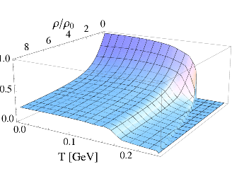
Figure 1: 3D-plot of the ratio $\bar{\sigma}/\sigma_{0}$ as a function of baryon density and temperature. Here Z/A=0.5

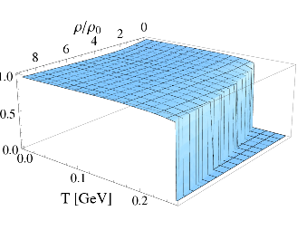
Figure 2: 3D-plot of the ratio $\bar{\phi}/\phi_{0}$ as a function of baryon density and temperature. Here Z/A=0.5

V Applications

The CDM code epa ; ind can be used for many applications since it allows to compute many useful quantities in a wide range of temperatures, baryon densities and isospin asymmetries. One of the most interesting applications is the study of chiral and scale phase transitions. To this purpose we used the code to build a phase diagram, as an extension of Fig. 8 of Ref. Bonanno and Drago (2009), by computing $\bar{\sigma}/\sigma_{0}$ (see Fig. 1) and $\bar{\phi}/\phi_{0}$ (see Fig. 2) as functions of T and $\rho_{B}$ in the case of isospin symmetric matter. Notice that at large temperatures $\bar{\sigma}/\sigma_{0}$ sharply decreases reaching a plateau where it assumes very small values. This plateau is a region where chiral symmetry is strongly restored, while scale invariance is still broken. When temperature becomes even larger scale invariance restores with a first order transition ($\bar{\phi}/\phi_{0}$ vanishes) , dragging together the restoration of chiral symmetry ($\bar{\sigma}/\sigma_{0}$ vanishes). The code allows also to study the role of the isospin in chiral and scale phase transitions.

It is necessary to point out that the results obtained here do not appear very different by those presented in Refs. Bonanno et al. (2007); Bonanno and Drago (2009) (although some differences are observed in the isospin splitting of the pion mass). The thermal fluctuation of the dilaton field, indeed, does not play a fundamental role. This is due to the value of the dilaton mass which remains large (about 1 GeV) also in the density-temperature region where the scale invariance restores.

In the future it would be interesting to include the hyperons in calculations, through an extension of the model in SU(3). This direction is actually explored by the Frankfurt group Dexheimer and Schramm (2008). The most interesting extension is the inclusion of the quark degrees of freedom, what will be done in the next works.

VI Acknowledgments

It is a pleasure to thank Alessandro Drago for his useful advices.

References

References

(1)
See EPAPS Document No. for the code cdm.f..
(2)
See http://df.unife.it/u/bonanno/CDM_code.zip.
Bonanno et al. (2007)
L. Bonanno,
A. Drago, and
A. Lavagno,
Phys. Rev. Lett. 99,
242301 (2007).
Bonanno and Drago (2009)
L. Bonanno and
A. Drago,
Phys. Rev. C79,
045801 (2009), eprint 0805.4188.
Senger (2004)
P. Senger, J.
Phys. G30, S1087
(2004).
Heide et al. (1994)
E. K. Heide,
S. Rudaz, and
P. J. Ellis,
Nucl. Phys. A571,
713 (1994).
Carter et al. (1996)
G. W. Carter,
P. J. Ellis, and
S. Rudaz,
Nucl. Phys. A603,
367 (1996).
Carter et al. (1997)
G. W. Carter,
P. J. Ellis, and
S. Rudaz,
Nucl. Phys. A618,
317 (1997).
Carter and Ellis (1998)
G. W. Carter and
P. J. Ellis,
Nucl. Phys. A628,
325 (1998).
Mocsy et al. (2004)
A. Mocsy,
I. N. Mishustin,
and P. J. Ellis,
Phys. Rev. C70,
015204 (2004).
Dexheimer and Schramm (2008)
V. Dexheimer and
S. Schramm
(2008), eprint arXiv:0802.1999 [astro-ph].