A numerical study of primordial magnetic field amplification by inflation-produced gravitational waves

Abstract

We numerically study the interaction of inflation-produced magnetic fields with gravitational waves, both of which originate from quantum fluctuations during inflation. The resonance between the magnetic field perturbations and the gravitational waves has been suggested as a possible mechanism for magnetic field amplification. However, some analytical studies suggest that the effect of the inflationary gravitational waves is too small to provide significant amplification. Our numerical study shows more clearly how the interaction affects the magnetic fields and confirms the weakness of the influence of the gravitational waves. We present an investigation based on the magnetohydrodynamic approximation and take into account the differences of the Alfven speed.

I Introduction

Recently, various observations have confirmed the presence of magnetic fields both in individual galaxies and on even larger scales such as in clusters of galaxies mag-obs . These magnetic fields have a typical strength of $10^{-6\sim-7}$G. Such large and strong magnetic fields are expected to have been amplified to their present levels by galactic dynamo theory dynamo-1 . However this efficiency is a matter of some debate, because this mechanism requires seed magnetic fields greater than $\sim 10^{-20}$G Giovannini and existing theories for generating seed fields do not achieve the required strength dynamo-2 . To fill the gap between observations and the dynamo theory, a large number of theoretical models have been suggested to generate stronger seed fields or to amplify the weak seed fields generated from existing theory. The minimum amplitude necessary in order for dynamo theory to produce the fields observed at the present epoch is estimated as approximately $10^{-34}$G at a comoving length of $10$kpc Davis .

In this paper, we focus on the amplification of inflation-produced magnetic fields by inflation-produced gravitational waves; a mechanism that was originally suggested by Tsagas (2003) Tsagas1 . Providing no exotic physics is assumed, inflation generally predicts quite small magnetic fields of roughly $10^{-53}$G Turner . Various mechanisms to break the conformal invariance of electrodynamics have been proposed to generate larger magnetic fields, but these are not widely accepted since they require the inclusion of new physics beyond the standard model. Gravitational generation of the massive Z-boson field has been suggested as a mechanism to naturally break conformal invariance within the standard model Davis ; Dimopoulos . However, the strength of the generated magnetic field with a reasonable model of field evolution is estimated to be only $10^{-29}$G on scales of $100$pc, which is not large enough to explain observations of the present day universe. Originally, Ref. Tsagas1 reported that such small seed magnetic fields may be amplified to the order of $10^{15}$ by amplification induced by gravitational waves. The key idea of this amplification mechanism is the resonance between gravitational waves and magnetic field waves as a result of the interaction between them, which occurs only when these have the same wavenumber. Since inflation generates both gravitational waves and magnetic fields at all scales, this mechanism is considered to be able to work on the inflationary magnetic fields. However, this work has since been revisited by several papers Betschart ; Zunckel ; Fenu which conclude that it does not provide such significant amplification.

In contrast to the majority of these studies, which have been performed analytically, we here tackle the problem with a numerical approach. The advantage of such a numerical study is that it enables us to accurately evaluate this effect under more realistic conditions. We numerically track the evolutionary history of the universe as it shifts from the radiation dominated era to the matter dominated era and finally to the cosmological constant dominated era. Since the universe is considered to have high conductivity after it becomes radiation dominated, we make use of the magnetohydrodynamic (MHD) approximation Zunckel . We take into account the Alfven velocity, which determines whether or not resonance amplification occurs in the MHD framework Marklund . In addition, numerical calculations allow us to follow the time evolution of the interaction process. We clearly show the behavior of the magnetic fields not only in both the long and short wavelength limits, but also at the point where each mode crosses the horizon, where the impact of the gravitational waves is the largest. Because of this property that the amplification is most efficient when the mode crosses the horizon, we only investigate the effect on magnetic fields produced by inflation which is the only mechanism that is able to generate such fields outside the horizon.

The outline of this paper is as follows. In Sec. II, we first introduce the basics of the covariant formalism which is convenient in describing the interaction between gravitational waves and magnetic fields. We then describe equations for the Hubble expansion, magnetic fields and gravitational waves, which form the base of our investigation. In Sec. III, we first arrange the equations to be applicable for our numerical calculation, and then perform the numerical calculation to evaluate the magnitude of the induced magnetic fields, and show and discuss the results. We end with our conclusions in Sec. IV.

II Basic equations

II.1 The covariant formalism

The interaction between magnetic fields and gravitational waves has been well studied using the covariant approach. We define the $1+3$ decomposition of space-time by choosing the time direction to be along the velocity vector of the fundamental observer $u_{a}$, which satisfies $u_{a}u^{a}=-1$. Then the observer’s rest frame is described by the projection tensor $h_{ab}=g_{ab}+u_{a}u_{b}$. Projecting the covariant derivative $\nabla_{a}$ onto the direction of $u_{a}$ and $h_{ab}$, we define the time derivative and the spatial derivative as $\dot{X}_{a\cdots b}\equiv u^{c}\nabla_{c}X_{a\cdots b}$ and $D_{c}X_{a\cdots b}\equiv{h_{c}}^{d}{h_{a}}^{e}\cdots{h_{b}}^{f}\nabla_{d}X_{e\cdots f}$, respectively. The 3-dimensional curl is defined as ${\rm curl}X_{a}\equiv\varepsilon_{abc}D^{b}X^{c}$, where $\varepsilon_{abc}$ is the antisymmetric permutation tensor.

In the covariant formalism, the basic kinematic quantities are defined by decomposing the covariant derivative of $u_{a}$,

$$\nabla_{b}u_{a}=\sigma_{ab}+\omega_{ab}+\frac{1}{3}\Theta h_{ab}-\dot{u}_{a}u_{b},$$ (1)

where $\sigma_{ab}=D_{(b}u_{a)}$, $\omega_{ab}=D_{[b}u_{a]}$, $\Theta=\nabla^{a}u_{a}=D^{a}u_{a}$ and $\dot{u}_{a}=u^{b}\nabla_{b}u_{a}$ are respectively the shear tensor, the vorticity tensor, the volume expansion scalar, and the 4-acceleration vector. Since we are interested in cosmological magnetic fields under the influence of gravitational waves in the expanding universe, we only consider the shear $\sigma_{ab}$ and the expansion $\Theta$, which correspond to the tensor perturbation and the Hubble expansion rate, respectively. Therefore, we neglect the vorticity $\omega^{ab}$ and acceleration fields $\dot{u}^{a}$ throughout this paper.

II.2 Background equation

For the evolution equation of the background space-time, we assume a spatially-flat Friedmann Robertson-Walker universe, for which the metric is given by $ds^{2}=-dt^{2}+a^{2}(t)\delta_{ij}dx^{i}dx^{j}$. In this metric space, the volume expansion scalar $\Theta$ is related to the scale factor $a(t)$ as $\Theta=3\dot{a}/a\equiv 3H$, where $H$ is the Hubble expansion rate and its evolution is simply given by the Friedmann equation,

$$H=H_{0}\sqrt{\Omega_{r}a^{-4}+\Omega_{m}a^{-3}+\Omega_{\Lambda}},$$ (2)

where we set $a(t_{0})=1$ and the subscript “0” denotes the present time. The density parameters $\Omega_{r}$, $\Omega_{m}$, $\Omega_{\Lambda}$ denote radiation, matter, and the cosmological constant, respectively. We use $\Omega_{r}h^{2}=4.15\times 10^{-5}$ and the WMAP 5 yr results $h=0.705$, $\Omega_{m}=0.274$, and $\Omega_{\Lambda}=0.726$ WMAP5yr .

II.3 Evolution equation for magnetic fields

The evolution equation for the magnetic field $B_{a}$ is derived by combining Maxwell’s equations Tsagas2 ,

$$\dot{E}_{\langle a\rangle}=\sigma_{ab}E^{b}-\frac{2}{3}\Theta h_{ab}E^{b}+{\rm curl}B_{a}-J_{\langle a\rangle},$$ (3)

$$\dot{B}_{\langle a\rangle}=\sigma_{ab}B^{b}-\frac{2}{3}\Theta h_{ab}B^{b}-{\rm curl}E_{a},$$ (4)

$$D^{a}E_{a}=\rho_{\rm e},$$ (5)

$$D^{a}B_{a}=0,$$ (6)

where $\rho_{\rm e}=-J_{a}u^{a}$ is the charge density and $J_{\langle a\rangle}\equiv h_{ab}J^{b}$ is the 3-dimensional current. If we neglect the effect of the matter components of the universe, $\rho_{\rm e}$ and $J_{\langle a\rangle}$ can be set to be zero. This enables us to obtain the evolution equation for the magnetic fields by only combining the Maxwell equations Tsagas1 ; Tsagas2 , resulting in a description of the propagation of magnetic field waves in vacuum.

However, the real universe is filled with charged particles, and therefore we need to take into account the electric current, which is given by Ohm’s law,

$$J_{\langle a\rangle}=\sigma(E_{a}+\varepsilon_{abc}v^{b}B^{c}),$$ (7)

where $\sigma$ denotes the electrical conductivity and $v_{a}$ is the plasma 3-velocity. After a large number of charged particles are produced at the time of reheating following inflation, the conductivity of the universe is considered to be high enough to assume $\sigma\rightarrow\infty$, which continues until today even after recombination of the universe Turner . In this limit, the MHD approximation is appropriate. In this paper, we also assume instantaneous reheating after inflation, allowing us to make use of the MHD approximation continuously throughout the numerical calculation.

The evolution equation for magnetic fields in the MHD approximation is derived by using Eq.(7) to replace $E_{a}$ by $J_{a}$ in the Maxwell equations Marklund . In the usual MHD limit, charge neutrality is assumed so that $\rho_{e}\approx 0$. Neglecting the second time derivative of $B_{a}$ and taking the limit $\sigma\rightarrow\infty$, we obtain

$$\dot{B}_{\langle a\rangle}+\frac{2}{3}\Theta B_{a}-\varepsilon_{abc}\varepsilon^{cde}B_{e}D^{b}v_{d}=\sigma_{ab}B^{b}.$$ (8)

The plasma 3-velocity in the third term satisfies the Euler equation,

$$\rho\left[\dot{v}_{\langle a\rangle}+v_{b}D^{b}v_{a}+\frac{1}{3}\Theta v_{a}+\sigma_{ab}v^{b}\right]=\varepsilon_{abc}J^{b}B^{c},$$ (9)

where $\rho$ is the total fluid energy density. Since the displacement current $\dot{E}^{a}$ is negligible compared to the electric current $J_{a}$ in the MHD limit, Eq.(3) becomes

$$J_{\langle a\rangle}={\rm curl}B_{a}.$$ (10)

Here, we have neglected the expansion term in Eq.(3), which is considered to be the same order as $\dot{E}^{a}$, and also the shear term, $\sigma_{ab}$, which is much smaller than the expansion $\Theta$. Linearizing and combining Eqs. (8), (9) and (10) yields an evolution equation for the magnetic fields expressed in terms of only the magnetic field variable $B$, Eqs. (26), (27) and (28). The detailed derivation of this expression is given in Sec. III.1.

II.4 Evolution equation for gravitational waves

In most previous work, the evolution of the gravitational waves is investigated using the evolution equation of $\sigma_{ab}$ Tsagas1 ; Betschart ; Zunckel ; Fenu . However, here we choose to use the variable $h_{ab}$ instead of $\sigma_{ab}$, since we have thoroughly investigated the evolution of the gravitational waves using $h_{ij}$ in our previous work Kuroyanagi . This variable is defined as the tensor perturbation in a spatially-flat Friedmann Robertson-Walker universe, $ds^{2}=-dt^{2}+a^{2}(t)(\delta_{ij}+h_{ij})dx^{i}dx^{j}$, and its evolution equation is given by the Einstein equation,

$$\ddot{h}_{ij}+3H\dot{h}_{ij}-\frac{1}{a^{2}}\nabla^{2}h_{ij}=0.$$ (11)

When considering only the transverse traceless components of $\sigma_{ab}$, which satisfy $D^{a}\sigma_{ab}=0$, $h_{ab}$ can be related to $\sigma_{ab}$ as ${\sigma_{a}}^{b}=\dot{h}_{a}{}^{b}/2$ Goode . Since $\sigma_{ab}$ is a first order variable, we therefore also treat $h_{ab}$ as first order.

Note that we have neglected the anisotropic stress term in Eq.(11), which is induced by magnetic fields in general Caprini . This effectively means we assume that the energy of the magnetic fields is negligibly small compared to that of the gravitational waves. This assumption is valid in the initial phase of our calculation, since we consider a situation in which the inflation-produced magnetic fields, which are generally small, are enhanced by the larger gravitational waves. However, after the power of the enhanced magnetic fields becomes comparable to the gravitational waves, the one-sided energy transfer from the gravitational waves to the magnetic fields may stop and the magnetic fields start to affect the evolution of the gravitational waves. Therefore, strictly speaking we need to take into account the effect of the anisotropic stress term if the energy of the magnetic fields grows to exceed that of the gravitational waves. However, since our primary aim in the present study is to ascertain whether the magnetic fields can be amplified to such a significant level at all, (i.e. to the degree suggested by Ref. Tsagas1 ), we are justified in ignoring the anisotropic stress term for the time being.

III Numerical calculation

III.1 Linearization and decomposition of the equations

Here, we rearrange the set of equations, Eqs. (8), (9) and (10), to a form suitable for numerical analysis, referring to the procedure of Ref. Marklund . For the numerical calculation, we use the linearized and decomposed equations. First, we linearize the equation by splitting the magnetic fields into a homogeneous background field $\tilde{B}$, which scales as $\dot{\tilde{B}}=-2\Theta\tilde{B}/3$, and the perturbed variables. In addition, we split the perturbed magnetic fields into parallel ${\cal B}_{a}$ and perpendicular ${\cal B}$ components.

$$B_{a}=\tilde{B}\left[(1+{\cal B})e_{a}+{\cal B}_{a}\right],$$ (12)

where ${\cal B}\equiv(e^{a}{B}_{a}-\tilde{B})/\tilde{B}$ and ${\cal B}_{a}\equiv N_{ab}B^{b}/\tilde{B}$. The spacelike unit vector $e^{a}$, which satisfies $e_{a}e^{a}=1$, is parallel to the background magnetic field $\tilde{B}$, and the projection tensor $N_{ab}=h_{ab}-e_{a}e_{b}$ is the metric of the hyper-surface orthogonal to $e^{a}$. In this paper, $\tilde{B}$ is treated as first order and ${\cal B}$ and ${\cal B}_{a}$ are second order. Note that the perturbed variables of the magnetic fields, ${\cal B}$ and ${\cal B}_{a}$, are normalized by the magnitude of the background magnetic field $\tilde{B}$. This means the linearized equations are valid as long as these values are much smaller than 1. We therefore have to be careful that the amplified fields do not exceed the background field, ${\cal B},{\cal B}_{a}>1$, in which case the linearization method is no longer applicable. Here, however, for similar reasons to those stated in Sec. II.4, we apply linearization as a first step since we are primarily interested in estimating whether the amplification is significant.

Similarly, we decompose the shear perturbation into three parts as

$${\sigma}_{ab}=\Sigma_{ab}+2\Sigma_{(a}e_{b)}+\left(e_{a}e_{b}-\frac{1}{2}N_{ab}\right)\Sigma,$$ (13)

where $\Sigma_{ab}\equiv(N_{(a}\!^{c}N_{b)}\!^{d}-N_{ab}N^{cd}/2){\sigma}_{cd}$, $\Sigma_{a}\equiv N_{ab}{\sigma}^{bc}e_{c}$ and $\Sigma\equiv{\sigma}_{ab}e^{a}e^{b}$. Furthermore we split the spatial derivative operator into $D_{\|}\equiv e^{a}D_{a}=d/dz$ and $D^{a}_{\perp}\equiv N^{ab}{\rm D}_{b}$.

Combining Eqs. (9) and (10) and neglecting second order terms of $v_{a}$ and $\sigma_{ab}$, we obtain

$$\dot{v}_{\langle a\rangle}+\frac{1}{3}\Theta v_{a}=\frac{1}{\rho}(B^{b}D_{b}B_{a}-B^{b}D_{a}B_{b}).$$ (14)

Taking the time derivative of Eq. (8),

$$\ddot{B}_{a}+\frac{2}{3}\dot{\Theta}B_{a}+\frac{2}{3}\Theta\dot{B}_{a}+B_{b}D^{b}\dot{v}_{a}-B_{a}D^{b}\dot{v}_{b}$$

$$-\frac{1}{3}\Theta B_{b}D^{b}v_{a}+\frac{1}{3}\Theta B_{a}D^{b}v_{b}+\dot{B}_{b}D^{b}v_{a}-\dot{B}_{a}D^{b}v_{b}$$

$$=\dot{\sigma}_{ab}B^{b}+\sigma_{ab}\dot{B}^{b},$$ (15)

where we neglect combinations of the spatial curvature ${\cal R}$ and $v_{a}$ since they are second order. We then substitute Eq. (14) into Eq. (15) and conduct the linearization by using Eqs. (12) and (13) and neglecting products of ${\cal B}$, ${\cal B}_{a}$ with first order variables, $\Sigma$, $\Sigma_{a}$ $\Sigma_{ab}$, ${\cal R}$ and $v_{a}$. This yields

$$(\ddot{\cal B}-\frac{2}{3}\Theta\dot{\cal B})e_{a}+(\ddot{\cal B}_{a}-\frac{2}{3}\Theta\dot{\cal B}_{a})+C_{A}^{2}[-D^{2}{\cal B}e_{a}$$

$$-(D_{\|}^{2}{\cal B}_{a}-D_{\perp a}D_{\|}{\cal B})]+\frac{4}{3}\Theta(e_{b}D^{b}v_{a}-e_{a}D^{b}v_{b})$$

$$=(\dot{\Sigma}-\frac{2}{3}\Theta\Sigma)e_{a}+(\dot{\Sigma}_{a}-\frac{2}{3}\Theta\Sigma_{a}),$$ (16)

where we define the Alfven velocity as $C_{A}^{2}\equiv\tilde{B}^{2}/\rho$. Here, we have used $\dot{\tilde{B}}=-2\Theta\tilde{B}/3$ and $\ddot{\tilde{B}}=-2\dot{\Theta}\tilde{B}/3+4\Theta^{2}\tilde{B}/9$. By linearizing Eq. (8), we obtain the equation to rewrite the term which includes $v_{a}$ in terms of the magnetic field variables and the gravitational wave variables,

$$e_{b}D^{b}v_{a}-e_{a}D^{b}v_{b}=\dot{\cal B}e_{a}+\dot{\cal B}_{a}-\Sigma e_{a}-\Sigma_{a}.$$ (17)

Substituting this and the relation $D_{\|}{\cal B}=-D_{\perp a}{\cal B}^{a}$, which comes from the constraint of Eq. (6), we obtain the equations for the parallel component to the direction of the background field $e^{a}$,

$$\ddot{\cal B}+\frac{2}{3}\Theta\dot{\cal B}-C_{A}^{2}D^{2}{\cal B}=\dot{\Sigma}+\frac{2}{3}\Theta\Sigma,$$ (18)

and for the perpendicular component,

$$\ddot{\cal B}_{a}+\frac{2}{3}\Theta\dot{\cal B}_{a}-C_{A}^{2}(D_{\|}^{2}{\cal B}_{a}+D_{\perp a}D_{\perp b}{\cal B}^{b})$$

$$=\dot{\Sigma}_{a}+\frac{2}{3}\Theta\Sigma_{a}.$$ (19)

Next, we decompose the equations by introducing the scalar harmonics $Q_{(k_{\perp})}$ which satisfy

$$D_{\perp}^{2}Q_{(k_{\perp})}=-\frac{k_{\perp}^{2}}{a^{2}}Q_{(k_{\perp})},$$ (20)

where $k_{\perp}$ is the physical wavenumber for the fields perpendicular to $e^{a}$. Taking the divergence and rotation of $Q_{(k_{\perp})}$, we define the vector harmonics of even and odd parity,

$$Q_{(k_{\perp})}^{a}=\left(\frac{k_{\perp}}{a}\right)^{-1}D_{\perp}^{a}Q_{(k_{\perp})},$$ (21)

$$\bar{Q}_{(k_{\perp})}^{a}=\left(\frac{k_{\perp}}{a}\right)^{-1}\epsilon^{a}\!_{b}D_{\perp}^{b}Q_{(k_{\perp})},$$ (22)

where $\epsilon^{ab}=\epsilon_{abc}e^{c}$. These harmonics satisfy $D_{\perp}^{2}Q_{(k_{\perp})}^{a}=-(k_{\perp}/a)^{2}Q_{(k_{\perp})}^{a}$ and $D_{\perp}^{2}\bar{Q}_{(k_{\perp})}^{a}=-(k_{\perp}/a)^{2}\bar{Q}_{(k_{\perp})}^{a}$. We then decompose the magnetic field variables in terms of the scalar and vector harmonics,

$${\cal B} = \sum_{k_{\perp}}{\cal B}_{(k_{\perp})}^{S}Q_{(k_{\perp})},$$

$${\cal B}^{a} = \sum_{k_{\perp}}\left({\cal B}_{(k_{\perp})}^{V}Q_{(k_{\perp})}^{a}+\bar{\cal B}_{(k_{\perp})}^{V}\bar{Q}_{(k_{\perp})}^{a}\right).$$ (23)

Similarly, the gravitational wave variables are expressed as

$$\Sigma = \sum_{k_{\perp}}\Sigma_{(k_{\perp})}^{S}Q_{(k_{\perp})},$$ (24)

$$\quad\Sigma^{a} = \sum_{k_{\perp}}\left(\Sigma_{(k_{\perp})}^{V}Q_{(k_{\perp})}^{a}+\bar{\Sigma}_{(k_{\perp})}^{V}\bar{Q}_{(k_{\perp})}^{a}\right).$$ (25)

We further decompose the variables by introducing the scalar harmonics for the parallel component $Q_{(k_{\|})}$, which satisfy $D_{\|}^{2}Q_{(k_{\|})}=-(k_{\|}/a)^{2}Q_{(k_{\|})}$. Then ${\cal B}^{S}_{(k_{\perp})}$ can be rewritten as ${\cal B}^{S}_{(k_{\perp})}=\sum_{k_{\|}}{\cal B}_{(k_{\perp},k_{\|})}^{S}Q_{(k_{\|})}$, similarly for ${\cal B}_{(k_{\perp})}^{V}$, $\bar{\cal B}_{(k_{\perp})}^{V}$, ${\Sigma}^{S}_{(k_{\perp})}$, ${\Sigma}^{V}_{(k_{\perp})}$, ${\bar{\Sigma}}^{V}_{(k_{\perp})}$. Hereafter, we drop subscripts $(k_{\perp},k_{\|})$. By applying the above decompositions, Eqs. (18) and (19) result in

$${\ddot{\cal B}}^{S}+\frac{2}{3}\Theta{\dot{\cal B}}^{S}+C_{A}^{2}\frac{k^{2}}{a^{2}}{\cal B}^{S}=\dot{\Sigma}^{S}+\frac{2}{3}\Theta\Sigma^{S},$$ (26)

similarly for ${\cal B}^{V}_{(k_{\perp})}$, and

$${\ddot{\bar{\cal B}}}\!\,^{V}+\frac{2}{3}\Theta{\dot{\bar{\cal B}}}\!\,^{V}+C_{A}^{2}\frac{k_{\|}^{2}}{a^{2}}{\bar{\cal B}}^{V}=\dot{\bar{\Sigma}}^{V}+\frac{2}{3}\Theta{\bar{\Sigma}}^{V}.$$ (27)

This is the final expression of the equation for the magnetic fields, which we use in our numerical calculation.

For the calculation of the evolution of the gravitational waves, we follow the procedure of our previous work Kuroyanagi . We use the Fourier transformed equation of Eq. (11),

$$\ddot{h}_{\bf k}^{\lambda}+3H\dot{h}_{\bf k}^{\lambda}+\frac{k^{2}}{a^{2}}h_{\bf k}^{\lambda}=0,$$ (28)

where $h_{ij}(x)=\sum_{\lambda=+,\times}\int d^{3}k(2\pi)^{-3/2}\epsilon_{ij}^{\lambda}(k)h_{\bf k}^{\lambda}(k)e^{i{\bf x}\cdot{\bf k}}$. The polarization tensors $\epsilon_{ij}^{+,\times}$ satisfy symmetric and transverse-traceless condition and are normalized as $\sum_{i,j}\epsilon_{ij}^{\lambda}(\epsilon_{ij}^{\lambda^{\prime}})^{*}=2\delta^{\lambda\lambda^{\prime}}$.

III.2 Method

Using Eqs. (2), (27) and (28), we numerically follow the evolution of both the magnetic fields and the gravitational waves under the influence of cosmic expansion. Although the magnetic field variables are decomposed into several parts, here for simplicity we first follow the evolution of the variable ${\bar{\cal B}}^{V}$. Strictly speaking all field components should be considered. However, since their amplitudes are thought to be approximately equal, one variable is sufficient to demonstrate the main result of this paper – that the final amplification is extremely small. The calculation begins at the early stage of the radiation dominated universe, from which the MHD approximation is valid until the present epoch. The initial condition of the induced magnetic field ${\bar{\cal B}}^{V}$ is set to be zero for all scales. Note that the variable ${\bar{\cal B}}^{V}$ is the value divided by background magnetic field $\tilde{B}$. This allows us to follow the evolution of the magnetic field without assuming the strength of the background field. It may not be reasonable to assume a homogeneous inflation-produced magnetic field as such fields are predicted to be a stochastic. However, as mentioned in Sec. II.4, our primary aim is to ascertain whether the magnetic fields can be amplified or not as suggested in Ref. Tsagas1 . Thus following their assumptions, we evaluate this effect under the simple situation of a homogeneous background field. In addition, although the considered situation is a little different, as the current term is neglected, the case of a stochastic magnetic field is investigated in detail analytically in Ref. Fenu . These authors also conclude that significant amplification does not occur.

The initial condition of the gravitational waves is derived from our numerical calculation presented in Ref. Kuroyanagi , which gives an almost scale-invariant power spectrum. We define the power spectrum of the gravitational waves as

$${\cal P}_{GW}=\frac{k^{3}}{2\pi^{2}}\sum_{\lambda=+,\times}|h_{\bf k}^{\lambda}|^{2}.$$ (29)

One may write the power spectrum of the gravitational waves generated outside the horizon during inflation as

$${{\cal P}}_{GW,{\rm prim}}(k)=\frac{16}{\pi}\left.\left(\frac{H}{m_{Pl}}\right)^{2}\right|_{k=aH}.$$ (30)

In our calculation, we assume chaotic inflation, meaning that CMB normalization gives $H_{\rm inf}/m_{pl}\sim 10^{-5.1}$. Here, the amplitude of the decomposed component ${\bar{\Sigma}}^{V}$ is assumed to contain the entire energy given in Eq. (30), which means we use ${\bar{\Sigma}}^{V}=\dot{h}^{\lambda}_{\bf k}$ assuming the two polarization states are equal. We also assume that it propagates in the direction of the background field, setting $k_{\rm grav}=k_{\|}$ in Eqs. (27) and (28). This assumption is in fact not strictly true for stochastic inflationary gravitational waves, meaning that the true amplitude may be a factor of a few smaller. However, this does not affect the result significantly.

III.3 Numerical results and discussion

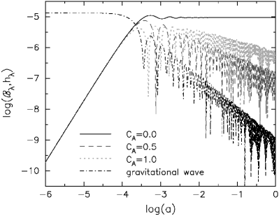
Figure 1: The evolution of ${\cal B}_{\lambda}\approx\sqrt{{\cal P}_{B}}$ shown with the scale factor $a$ as the horizontal axis. Here, we show the mode with wavenumber $k/a_{0}H_{0}=10^{2}$. The solid curve shows the case where $C_{A}=0.0$, the dashed curve shows $C_{A}=0.5$, and the dotted curve shows $C_{A}=1.0$. Additionally, the dot-dashed line shows the evolution of the gravitational wave mode $h_{\lambda}=\sqrt{{\cal P}_{GW}}$.

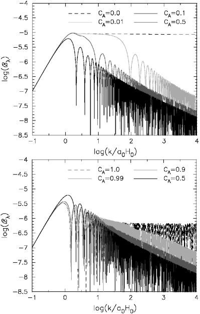
Figure 2: The square root of the power spectrum of the induced magnetic fields ${\cal B}_{\lambda}=\sqrt{{\cal P}_{B}}$ at the present time. The horizontal axis is the wavenumber normalized at the present horizon scale ($\sim 1/a_{0}H_{0}$). The upper panel shows the small Alfven speed case, $C_{A}=0.0,0.01,0.1,0.5$, and the bottom panel shows the large Alfven speed case, $C_{A}=0.5,0.9,0.99,1.0$

We first show the time evolution of the square root of the power spectrum in Fig. 1, which is defined as

$${\cal P}_{B}=\frac{k^{3}}{2\pi^{2}}|{\bar{\cal B}}^{V}|^{2}.$$ (31)

This can be interpreted as the power of the induced magnetic field perturbation with characteristic scale $\lambda=2\pi/k$, ${\cal B}_{\lambda}\approx\sqrt{{\cal P}_{B}}$. In this figure, we show the mode with wavenumber $k=10^{2}/a_{0}H_{0}$ for three cases of different Alfven speeds, $C_{A}=0.0,0.5,1.0$. Since the energy density of the magnetic fields is much smaller than the total energy density of the universe, the real universe is considered to be close to the case $C_{A}=0.0$. We also plot the evolution of the gravitational wave mode $h_{\lambda}\approx\sqrt{P_{GW}}$. As seen in the figure, the largest amplification occurs at around the point at which a mode enters the horizon, when the magnetic fields are amplified to the same power as the gravitational waves. After the mode enters the horizon, its behavior depends on the value of the Alfven speed. For $C_{A}=0.0$, the induced magnetic field maintains a constant amplitude, while for $C_{A}=0.5$ and $1.0$, the induced field undergoes oscillatory decay, with a decay rate that depends on the Alfven speed.

According to Eq. (27), the behavior described above can be interpreted as follows. When the mode is outside the horizon $k\ll aH$, the evolution of the magnetic fields depends on the amplitude of the gravitational waves as $\dot{B}_{\bf k}\propto\Sigma_{\bf k}$. At the same time, the gravitational waves remain at constant amplitude when they are outside the horizon, $\Sigma_{\bf k}\sim\dot{h}_{\bf k}\sim 0$. This means the magnetic fields are barely induced at all by those gravitational waves outside the horizon. However, when the mode becomes comparable to the horizon scale ($k\sim aH$), where the gravitational waves begin to oscillate, $\Sigma_{\bf k}$ becomes larger and induces magnetic field perturbations. This is the reason that the magnetic field perturbation is seen to increase toward the time of horizon crossing in Fig. 1.

The evolution inside the horizon $k\gg aH$ depends on the value of the Alfven speed. Setting the Alfven velocity to zero is equivalent to saying there is no Alfven mode. Thus, the resonant amplification and the decay of oscillating waves due to cosmic expansion do not occur. This is the reason why the evolution of the magnetic field fluctuations in the case $C_{A}=0.0$ is flat after entering the horizon in Fig. 1. In this case, the amplitude of the induced magnetic field is determined only by the amplitude of the gravitational waves at their horizon crossing. In contrast, if the Alfven mode exists, $C_{A}\neq 0.0$, the magnetic field starts to oscillate after entering the horizon. In this case, the equation of the magnetic field takes the form of a forced oscillator sourced by the gravitational wave. In the case where the velocities of the magnetic field mode and the gravitational wave mode are the same, i.e. the case of $C_{A}=1.0$, resonant oscillation occurs and pushes up the amplitude of the magnetic field perturbation. On the other hand, cosmic expansion reduces the energy of the oscillating magnetic waves at a rate proportional to $a^{-1/2}$ and the gravitational waves at a rate proportional to $a^{-1}$. Since the gravitational waves decay faster than the magnetic field perturbations, the amplification effect by resonance oscillation becomes weaker as the universe evolves. Therefore, as seen in Fig. 1, the magnetic field perturbations decay after they enter the horizon even when the resonant condition is satisfied.

Figure 2 shows the square root of the power spectrum at the present time for several different values of the Alfven speed. We see that the induced magnetic fields are the largest in the case of $C_{A}=0.0$. In this case, as mentioned above, there is no resonant amplification and no decay of the amplitude due to the cosmic expansion after the horizon crossing, so the amplitude of the induced magnetic field only depends on the that of the gravitational waves at the horizon crossing. Since the primordial power spectrum of the gravitational waves is scale-invariant, the power spectrum of the induced magnetic fields also ends up scale-invariant. On the other hand, in the other cases where the Alfven speed is not zero, the magnetic fields suffer damping due to the cosmic expansion after they enter the horizon. As seen in the upper panel of Fig. 2, the damping arises on modes smaller than $aH/C_{A}$. In the bottom panel, which shows the cases where the Alfven speed is large enough to bring on the resonance with the gravitational waves, we see the amplification pushes up the amplitude of the smaller modes. The change in the frequency dependence seen around $k/a_{0}H_{0}\sim 10^{1.3}$ is considered to be due to the change of the Hubble expansion rate at matter-radiation equality, which causes the change of the frequency dependence of the amplitude of the source term (gravitational waves). In any case, the magnitude of the induced magnetic field is less than $10^{-5}$ times the magnitude of the original background field at all scales, which leads us to conclude that the impact of the gravitational waves is negligibly small.

IV Conclusion

We have numerically estimated how primordial magnetic fields are affected by inflation-produced gravitational waves in the framework of the MHD approximation. Our calculation has shown that the magnetic fields gain most energy from the gravitational waves when each mode enters the horizon, although the impact is not large enough to call it “amplification”. We have found that the magnitude of the induced magnetic field is less than $10^{-5}$ times the magnitude of the original background field. This conclusion is consistent with the analytical estimation in the previous work of Ref. Betschart ; Zunckel ; Fenu .

Although the induced magnetic fields are quite small in all cases, we have found that the Alfven speed makes a difference to the evolution of the magnetic fields inside the horizon. The Alfven speed is the factor which determines whether resonance amplification occurs or not, and we find that it occurs when the Alfven speed is the same as the speed of light. However, this situation would not be seen in the real universe, because such a large Alfven speed corresponds to a situation in which the magnetic fields dominate the energy density of the universe. Furthermore, even if we assume this unrealistic situation, our investigation has found that the amplitude of the induced magnetic fields does not increase because both the magnetic field waves and the gravitational waves lose their energy via the cosmic expansion after they enter the horizon. On the other hand, if the Alfven speed is negligibly small, the induced magnetic field does not decay, which results in a larger amplification rate compared to the case of finite Alfven speed.

One thing we must note is that our calculation does not take into account the epoch before reheating, where the conductivity of the universe is low, and the epoch during reheating, where the Hubble expansion rate behaves as in a matter dominated universe. When the conductivity is low, we cannot apply the MHD equations we have used in this paper. However, we do not think the magnetic fields are significantly affected by the gravitational waves during the low conductivity epoch, because most of the modes we observe today are outside the horizon during the early epoch, and the gravitational waves maintain a constant amplitude. Although the equation for magnetic fields in a vacuum is different from that of the MHD limit, the source term consists of the same components, namely the time derivatives of the gravitational waves, $\sigma_{a}^{b}=\dot{h}_{a}^{b}/2$ and $\dot{\sigma}_{a}^{b}$ (see Eq. (3) of Ref. Tsagas1 ). Thus, the gravitational waves barely induce the magnetic fields outside the horizon, even if the conductivity is low in the early epoch. Also, the change in the Hubble expansion rate does not affect the behavior of the constant gravitational waves when they are outside the horizon. Therefore, the early epoch before and during reheating is considered to not change our results.

References

- (1) A. M. Wolfe, K. M. Lanzetta, and A. L. Oren, Astrophys. J. 388, 17 (1992); T. E. Clarke, P. P. Kronberg, and H. Boehringer, Astrophys. J. 547, L111 (2001); L. M. Widrow, Rev. Mod. Phys. 74, 775 (2002); Y. Xu, P. P. Kronberg, S. Habib, and Q. W. Dufton, Astrophys. J. 637, 19 (2006); P. P. Kronberg et al. Astrophys. J. 676, 7079 (2008).
- (2) A. Brandenburg and K. Subramanian, Phys. Rep. 417, 1 (2005).
- (3) M. Giovannini, Int. J. Mod. Phys. D 13, 391 (2004).
- (4) R. Kulsrud et al., Phys. Rep. 283, 213 (1997).
- (5) A. C. Davis, K. Dimopoulos, T. Prokopec and O. Trnkvist, Phys. Lett. B 501, 165 (2001).
- (6) C. G. Tsagas, P. K. S. Dunsby and M. Marklund, Phys. Lett. B 561, 17 (2003); C. G. Tsagas, Phys. Rev. D 72, 123509 (2005); Phys. Rev. D 75, 087901 (2007).
- (7) M. S. Turner and L. M. Widrow, Phys. Rev. D 37, 2743 (1988).
- (8) K. Dimopoulos, T. Prokopec, O. Tornkvist and A-C. Davis, Phys. Rev. D 65, 063505 (2002).
- (9) G. Betschart, C. Zunckel, P. K. S. Dunsby and M. Marklund, Phys. Rev. D 72, 123514 (2005); Phys. Rev. D 75, 087902 (2007).
- (10) C. Zunckel, G. Betschart, P. K. S. Dunsby and M. Marklund, Phys. Rev. D 73, 103509 (2006).
- (11) E. Fenu and Ruth Durrer, Phys. Rev. D 79, 024021 (2009).
- (12) M. Marklund and C. Clarkson, Mon. Not. Roy. Astron. Soc. 358, 892 (2005).
- (13) E. Komatsu, et al., Astrophys. J. Suppl. 180, 330 (2009).
- (14) C. G. Tsagas, Classical and Quantum Gravity 22, 393 (2005).
- (15) S. Kuroyanagi, T. Chiba and N. Sugiyama, Phys. Rev. D 79, 103501 (2009).
- (16) S. W. Goode, Phys. Rev. D 39, 2882 (1989).
- (17) C. Caprini and R. Durrer, Phys. Rev. D 65, 023517 (2001); Phys. Rev. D 74, 063521 (2006); C. Caprini, R. Durrer and G. Servant, arXiv:0909.0622 [astro-ph.CO].