Gravitomagnetic corrections on gravitational waves

Abstract

Gravitational waveforms and production could be considerably affected by gravitomagnetic corrections considered in relativistic theory of orbits. Beside the standard periastron effect of General Relativity, new nutation effects come out when ${\displaystyle c^{-3}}$ corrections are taken into account. Such corrections emerge as soon as matter-current densities and vector gravitational potentials cannot be discarded into dynamics. We study the gravitational waves emitted through the capture, in the gravitational field of massive binary systems (e.g. a very massive black hole on which a stellar object is inspiralling) via the quadrupole approximation, considering precession and nutation effects. We present a numerical study to obtain the gravitational wave luminosity, the total energy output and the gravitational radiation amplitude. From a crude estimate of the expected number of events towards peculiar targets (e.g. globular clusters) and in particular, the rate of events per year for dense stellar clusters at the Galactic Center (SgrA^∗), we conclude that this type of capture could give signatures to be revealed by interferometric GW antennas, in particular by the forthcoming laser interferometer space antenna LISA.

I Introduction

Searching for signatures of gravitational waves (GWs) and achieving a suitable classification of emitting sources have become two crucial tasks in GW-science. In fact, the today sensitivity levels and theoretical developments are leading toward a general picture of GW-phenomena which could not be possible in the previous pioneering era. Experimentally, several GW ground-based-laser-interferometer detectors ($10^{-1}kHz$) have been built in the United States (LIGO) Abra , Europe (VIRGO and GEO) Caron ; Luck and Japan (TAMA) Ando , and are now taking data at designed sensitivities. A laser-interferometer space antenna (LISA) LISA ($10^{-4}\sim 10^{-2}Hz$) might fly within the next decade.

From a theoretical point of view, recent years have been characterized by numerous major advances due, essentially, to the development of numerical gravity. Concerning the most promising sources to be detected, the GW generation problem has improved significantly in relation to the dynamics of binary and multiple systems of compact objects as neutron stars and black holes. Besides, the problem of non-geodesic motion of particles in curved spacetime has been developed considering the emission of GWs Poisson ; Mino . Solving these problems is of considerable importance in order to predict the accurate waveforms of GWs emitted by extreme mass-ratio binaries, which are among the most promising sources for LISA Finn .

From a more genuine astrophysical viewpoint, observations towards the central regions of galaxies have detected peculiar compact massive objects which are present in almost all observed galaxies. The occurrence of such systems has been revealed thanks to the advance in high angular resolution instrumentation for a wide range of electromagnetic wavelengths. Space-telescopes as HST or ground-based telescope, which use adaptive optics, have been extremely useful for studying kinematics of galactic internal regions reaching accuracy of mill-pc for the Milky Way and of pc-fractions for external galaxies. The main conclusion of all these studies is that the central region of most of galaxies is dominated by large compact objects with masses of the order $M\simeq 10^{6}\div 10^{9}M_{\odot}$. In the case of Milky Way, the peculiar object in the Sagittarius region (SgrA^∗) is of the order $M\simeq 3\times 10^{6}M_{\odot}$ and it is usually addressed as a massive black hole (MBH), also if its true physical nature is far to be finally identified viollier ; pla .

In any case, a deep link exists between the central MBH and the geometrical, kinematical and dynamical features of the host galaxy. In particular, the MBH is correlated with the global shape of galactic spheroid, with the velocity dispersion of surrounding stars, with the mean density and the total mass of the host galaxy. Dynamics of stars moving around the MBH has a series of interesting characteristics which are of extreme interest for GW detection and production. Due to this occurrence, searching for GWs coming from objects interacting with MBHs is a major task for GW interferometry from space and ground-based experiments.

In this paper, we are going to study the evolution of compact binary systems, formed through the capture of a moving (stellar) mass $m$ by the gravitational field, whose source is a massive MBH of mass $M$ where $m\ll M$. One expects that small compact objects ($1\div 20M_{\odot}$) from the surrounding stellar population will be captured by these black holes following many-body scattering interactions at a relatively high rate Sigurdsson ; Sigurdsson2 . It is well known that the capture of stellar-mass compact objects by massive MBHs could constitute, potentially, a very important target for LISA Danzmann ; freitag . However, dynamics has to be carefully discussed in order to consider and select all effects coming from standard stellar mass objects inspiralling over MBHs.

In a previous paper Capoz , we have shown that, in the relativistic weak field approximation, when considering higher order corrections to the equations of motion, gravitomagnetic effects in the theory of orbits, can be particularly significant, leading also to chaotic behaviors in the transient regime dividing stable from unstable trajectories. Generally, such contributions are discarded since they are considered too small. However, in a more accurate analysis, this is not true and gravitomagnetic corrections could give peculiar characterization of dynamics.

In Capoz , Newtonian and relativistic theories of orbits have been reviewed considering, in particular, how relativistic corrections affect the ”classical” orbits binney ; landau . Equations of motion and phase portraits of solutions indicate that, beside the standard periastron precession at order $c^{-2}$, new nutation effects come out at order $c^{-3}$ and it is misleading to neglect them.

According to these effects, orbits remain rather eccentric until the final plunge, and display both extreme relativistic perihelion precession and Lense-Thirring Thirring1 ; Thirring ; iorio precession of the orbital plane due to the spin of MBH, as well as orbital decay. In Ryan , it is illustrated how the measured GW-waveforms can effectively map out the spacetime geometry close to the MBH. In DeLaurentis ; nucita , the classical orbital motion (without relativistic corrections in the motion of the binary system) has been studied in the extreme mass ratio limit $m\ll M$, assuming the stellar system density and richness as fundamental parameters. The conclusions have been that $i)$ the GW-waveforms have characterized by the orbital motion (in particular, closed or open orbits give rise to very different GW-production and waveform shapes); $ii)$ in rich and dense stellar clusters, a large production of GWs can be expected, so that these systems could be very interesting for the above mentioned ground-based and space detectors; $iii)$ the amplitudes of the strongest GW signals are expected to be roughly an order of magnitude smaller than LISA’s instrumental noise.

In this paper, we investigate the GW emission by binary systems, in the extreme mass ratio limit, by the quadrupole approximation, considering orbits affected by both nutation and precession effects, taking into account also gravitomagnetic terms in the weak field approximation of the metric. We will see that gravitational waves are emitted with a ”peculiar” signature related to the orbital features: such a signature may be a ”burst” wave-form with a maximum in correspondence to the periastron distance or a modulated waveform, according to the orbit stability. Here we face this problem discussing in detail the dynamics of such a phenomenon which could greatly improve the statistics of possible GW sources.

Besides, we give estimates of the distributions of these sources and their parameters. It is worth noticing that the captures occur when objects, in the dense stellar cusp surrounding a galactic MBH, undergo a close encounter, so that the trajectory becomes tight enough that orbital decay through emission of GWs dominates the subsequent evolution. According to Refs. Cutler1 ; Cutler2 ), for a typical capture, the initial orbital eccentricity is extremely large (typically $1-e\sim 10^{-6}{-}10^{-3}$) and the initial pericenter distance very small ($r_{\rm p}\sim 8-100M$, where $M$ is the MBH mass FreitagApJ . The subsequent orbital evolution may (very roughly) be divided into three stages. In the first and longest stage the orbit is extremely eccentric, and GWs are emitted in short “pulses” during pericenter passages. These GW pulses slowly remove energy and angular momentum from the system, and the orbit gradually shrinks and circularizes. After $\sim 10^{3}-10^{8}$ years (depending on the two masses and the initial eccentricity) the evolution enters its second stage, where the orbit is sufficiently circular: the emission can be viewed as continuous. Finally, as the object reaches the last stable orbit, the adiabatic inspiral transits to a direct plunge, and the GW signal cuts off. Radiation reaction quickly circularizes the orbit over the inspiral phase; however, initial eccentricities are large enough that a substantial fraction of captures will maintain high eccentricity until the final plunge. It has been estimated Cutler1 that about half of the captures will plunge with eccentricity $e\gtrsim 0.2$. While individually-resolvable captures will mostly be detectable during the last $\sim 1-100$ yrs of the second stage (depending on the stellar mass $m$ and the MBH mass), radiation emitted during the first stage will contribute significantly to the confusion background. As we shall see, the above scenario is heavily modified since the gravitomagnetic effects play a crucial role in modify the orbital shapes that are far from being simply circular or elliptic and no longer closed.

The layout of the paper is the following. In Sect.II, we give a summary of gravitomagnetic corrections to the metric showing how the geodesic equation results modified by their presence. Besides we study in details orbits with such corrections showing the phase portraits and the velocity fields determined by the motion of mass $m$ around the MBH. The GW-luminosity in the quadrupole approximation is discussed in Sect.III while GW-amplitude with gravitomagnetic corrections is discussed in Sect.IV giving also a resume of numerical results. Rate and event number estimations are given in Sect.V. Conclusions are drawn in Sect.VI.

II Gravitomagnetic corrections

In a previous paper Capoz , we studied how the relativistic theory of orbits for massive point-like objects is affected by gravitomagnetic corrections. In particular, we considered the corrections on the orbits of higher-order terms in $v/c$ and this is the main difference with respect to the standard gravitomagnetic effect discussed so far where corrections are taken into account only in the weak field limit and not on the geodesic motion. The problem of gravitomagnetic vector potential, entering into the off-diagonal components $g_{0l}$ of the metric $g_{\mu\nu}$, can be greatly simplified and the corrections can be seen as further powers in the expansion in $c^{-1}$ (up to $c^{-3}$). Nevertheless, the effects on the orbit behavior are interesting and involve not only the precession at periastron but also nutation corrections. Here we briefly recall such previous result sending to Capoz for a detailed analysis.

The metric, in weak field limit where gravitomagnetic corrections are present, is:

$$ds^{2}=\left(1+\frac{2\Phi}{c^{2}}\right)c^{2}dt^{2}-\frac{8\delta_{lj}V^{l}}{c^{3}}cdtdx^{j}-\left(1-\frac{2\Phi}{c^{2}}\right)\delta_{lj}dx^{i}dx^{j}\;,$$ (1)

where the gravitational Newtonian potential $\Phi(x)$ is

$$\Phi(x)=-G\int\frac{\rho}{\left|\mathbf{x}-\mathbf{x}^{\prime}\right|}d^{3}x^{\prime}\;,$$ (2)

and the vector potential $V^{l}$ is

$$V^{l}=-G\int\frac{\rho v^{l}}{\left|\mathbf{x}-\mathbf{x}^{\prime}\right|}d^{3}x^{\prime}\;,$$ (3)

given by the matter current density $\rho v^{l}$ of the moving bodies. This last potential gives rise to the gravitomagnetic corrections.

It is clear that the approximation is up to $c^{-3}$ in the Taylor expansion. From Eq.(1), it is straightforward to construct a variational principle from which the geodesic equation follows. Then we can derive the orbital equations. As standard, we have

$$\ddot{x}^{\alpha}+\Gamma_{\mu\nu}^{\alpha}\dot{x}^{\mu}\dot{x}^{\nu}=0\;,$$ (4)

where dot indicates the differentiation with respect to the affine parameter. In order to put in evidence the gravitomagnetic contributions, let us explicitly calculate the Christoffel symbols at lower orders. By some straightforward calculations, one gets

$$\begin{array}[]{cl}\Gamma^{0}_{00}&=0\\ \Gamma^{0}_{0j}&=\frac{1}{c^{2}}\frac{\partial\Phi}{\partial x^{j}}\\ \Gamma^{0}_{ij}&=-\frac{2}{c^{3}}\left(\frac{\partial V^{i}}{\partial x^{j}}+\frac{\partial V^{j}}{\partial x^{i}}\right)\\ \Gamma^{k}_{00}&=\frac{1}{c^{2}}\frac{\partial\Phi}{\partial x^{k}}\\ \Gamma^{k}_{0j}&=\frac{2}{c^{3}}\left(\frac{\partial V^{k}}{\partial x^{j}}-\frac{\partial V^{j}}{\partial x^{k}}\right)\\ \Gamma^{k}_{ij}&=-\frac{1}{c^{2}}\left(\frac{\partial\Phi}{\partial x^{j}}\delta^{k}_{i}+\frac{\partial\Phi}{\partial x^{i}}\delta^{k}_{j}-\frac{\partial\Phi}{\partial x^{k}}\delta_{ij}\right)\end{array}$$ (5)

In the approximation which we are going to consider, we are retaining terms up to the orders $\Phi/c^{2}$ and $V^{j}/c^{3}$. It is important to point out that we are discarding terms like $(\Phi/c^{4})\partial\Phi/\partial x^{k}$, $(V^{j}/c^{5})\partial\Phi/\partial x^{k}$, $(\Phi/c^{5})\partial V^{k}/\partial x^{j}$, $(V^{k}/c^{6})\partial V^{j}/\partial x^{i}$ and of higher orders. Our aim is to show that, in several cases like in tight binary stars, it is not correct to discard higher order terms in $v/c$ since physically interesting effects could come out. A vector equation for the spatial components of geodesics accounting for the gravitomagnetic effects is Capoz :

$$\frac{d\mathbf{e}}{dl_{euclid}}=-\frac{2}{c^{2}}\left[\nabla\Phi-\mathbf{e}(\mathbf{e}\cdot\nabla\Phi)\right]+\frac{4}{c^{3}}\left[\mathbf{e}\wedge(\nabla\wedge\mathbf{V})\right]\,.$$ (6)

The gravitomagnetic term is the second in Eq.(6) and it is usually discarded since considered not relevant. This is not true if $v/c$ is quite large as in the cases of tight binary systems or point masses approaching to black holes. Orbits, corrected by such effects can be explicitly achieved.

II.1 Orbits with gravitomagnetic corrections

Orbits with gravitomagnetic effects can be obtained starting from the classical theory and then correcting it by successive relativistic terms. In Capoz , it is shown that, taking into account the gravitomagnetic terms, in the weak field approximation and in the extreme mass-ratio limit $m\ll M$, one obtains a motion with precession and nutation by solving numerically the Euler-Lagrange equations. It is possible to obtain the parametric orbital equations of a massive particle starting from a variational principle where the canonical Lagrangian is derived by the metric (1). Being $\frac{\partial\mathcal{L}}{\partial t}=0$, we have $\frac{d}{dt}\left[\frac{\partial\mathcal{L}}{\partial\dot{t}}\right]=0$ and then $\frac{\partial\mathcal{L}}{\partial\dot{t}}=E$ where $E$ is a constant that can be interpreted as an energy per mass unit. Owing to the dependence of the Lagrangian from $\theta$ and $\phi$, we have, in general, $\frac{\partial\mathcal{L}}{\partial\phi}\neq 0$ and, furthermore, considering the initial conditions $\theta=\frac{\pi}{2}$ and $\dot{\theta}=0$ we have $\ddot{\theta}\neq 0$. This means, by straightforward calculations,

$$\ddot{\theta}=\frac{4c^{3}\text{E}GMr\dot{r}-16\cos G^{2}M^{2}\phi\left(\dot{r}\right)^{2}-16G^{2}M^{2}\sin\phi\left(\dot{r}\right)^{2}-16\cos G^{2}M^{2}r\phi\dot{r}\dot{\phi}+16G^{2}M^{2}r\sin\phi\dot{r}\dot{\phi}}{r^{2}+c^{6}r^{4}-4c^{2}G^{2}M^{2}\,.}$$ (7)

As it is possible to see from Eq.(7), planar motion is possible setting the initial condition $\dot{r}=0$, i.e. for the particular case of circular orbits; otherwise orbital motions present precession and nutation corrections. Giving explicitly the energy first integral

$$\dot{t}=\frac{1}{c^{3}r-2cG\mu}\left.\Big{\{}-4G\mu(\cos\theta+\sin\theta(\cos\phi+\sin\phi))\dot{r}+r\left.\Big{[}c^{3}E-4G\mu\left((-\sin\theta+\cos\theta(\cos\phi+\sin\phi))\dot{\theta}\right.\right.\right.$$ (8)

$$\left.\left.+\sin\theta(\cos\phi-\sin\phi)\dot{\phi}\right.)\Big{]}\right.\Big{\}}\,,$$

and the Euler-Lagrange equations (where the energy first integral can be suitably substituted) we get the differential system

$$\ddot{r}=\frac{1}{cr\left(rc^{2}+2G\mu\right)}\Big{[}c\left(rc^{2}+G\mu\right)\left(\dot{\theta}^{2}+\sin^{2}\theta\dot{\phi}^{2}\right)r^{2}$$ (9)

$$-4G\mu\dot{t}\left((\cos\theta(\cos\phi+\sin\phi)-\sin\theta)\dot{\theta}+\sin\theta(\cos\phi-\sin\phi)\dot{\phi}\right)r+cG\mu\dot{r}^{2}-cG\mu\dot{t}^{2}\Big{]}\,,$$

$$\ddot{\phi}=-\frac{2\left(c\cot\theta\left(rc^{2}+2G\mu\right)\dot{\theta}\dot{\phi}r^{2}+\dot{r}\left(2G\mu\csc\theta(\sin\phi-\cos\phi)\dot{t}+cr\left(rc^{2}+G\mu\right)\dot{\phi}\right)\right)}{r^{2}\left(rc^{3}+2G\mu c\right)}\,,$$ (10)

$$\ddot{\theta}=\frac{c\cos\theta r^{2}\left(rc^{2}+2G\mu\right)\sin\theta\dot{\phi}^{2}+\dot{r}\left(4G\mu(\cos\theta(\cos\phi+\sin\phi)-\sin\theta)\dot{t}-2cr\left(rc^{2}+G\mu\right)\dot{\theta}\right)}{r^{2}\left(rc^{3}+2G\mu c\right)}\,.$$ (11)

Such a system is highly non linear. For its solution, we have to adopt numerical methods. The main characteristics of solutions can be evaluated seeing at Fig.1 where the stiffness of the system is evident.

From Eqs.(9)-(11), it is clear that additional terms appear with respect to the classical Newtonian motion. Such corrections are not independent from $\phi$ and $\theta$. Obviously, these terms become important as soon as velocities approach relativistic regimes and the ratio ${\displaystyle\frac{v}{c}}$ is quite large. In some physical situations, e.g. in extreme dense globular clusters or around the Galactic Center, such a ratio can be in the range $10^{-2}\div 10^{-3}$ being not negligible at all (see freitag and references therein).

In Fig.1, we have shown the trend of $\ddot{r}$, $\ddot{\phi}$, $\ddot{\theta}$, as function of $t$, and $\ddot{\theta}_{NO}$ which is the trend without gravitomagnetic correction. It can be seen that this last plot gives deviation from zero that are essentially null, confirming the planarity of orbital motions in absence of gravitomagnetic corrections (the differences have at least four orders of magnitude between $\ddot{\theta}_{NO}(t)$ and $\ddot{\theta}(t)$).

To have a further insight of the gravitomagnetic correction relevance on the relativistic orbital motion, we have derived a numerical solution with the following parameters and initial conditions: ${\displaystyle\mu=\frac{mM}{m+M}\cong 1.4M_{\odot}}$, $r_{0}=500\mu$, $E=0.95$, $\phi_{0}=0$, $\theta_{0}=\frac{\pi}{2}$, $\dot{\phi_{0}}=-\frac{1}{10}\dot{r}_{0}$ and $\dot{r}_{0}=-\frac{1}{100}c$. In Fig.(2), we have plotted $\theta_{NO}(t)-\frac{\pi}{2}$ without gravitomagnetic corrections and $\theta_{Grav}(t)-\frac{\pi}{2}$, with gravitomagnetic corrections. In the bottom panel, there is, starting from the left to the right, the trend of the difference between the orbital radii $r_{Grav}$ and $r_{NO}$ with and without gravitomagnetic corrections respectively; we plotted also the differences $r_{Grav}-r_{NO}$ and $t_{Grav}-t_{NO}$(red lines) and the ratio between coordinated time ${\displaystyle\frac{t_{Grav}}{\tau}}$ versus proper time $\tau$ (blue line). It is interesting to see the discrepancy from $\frac{\pi}{2}$ of $\theta$ with and without the gravitomagnetic effect. It is evident that we have planar orbital motion in the Newtonian case, whilst, in presence of gravitomagnetic corrections, there is a tendency to precession and nutation of the orbital plane which give rise, orbit by orbit, to cumulative effects (a difference of five orders of magnitude between $z_{NO}(t)$ and $z_{Grav}(t)$ can be evaluated). At the beginning, the effect is very small but, orbit by orbit, it grows and, for a suitable interval of time, the effect cannot be neglected [see Fig.(3), left bottom panel in which the differences in $x$ and $y$ are shown starting from the initial orbits up to the last ones by step of about 1500 orbits). On the bottom right, it is shown the basic orbit. For about 4850 orbits and a time interval of about $1.7$ years, we found that the differences in coordinated time, computed with and without gravitomagnetic effects, are increasing as well as the differences in $x$, $y$ and $z$ coordinates. See also Fig. (4) in which we show the differences between the gravitational wave strain amplitude computed with and without the gravitomagnetic orbital corrections (see the discussion in forthcoming Sect. IV).

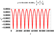
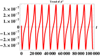
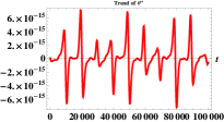
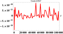
Figure 1: Plots of $\ddot{r}=\ddot{r}(t)$(left upper panel),$\ddot{\phi}=\ddot{\phi}(t)$ (right upper panel), $\ddot{\theta}=\ddot{\theta}(t)$(left bottom panel),$\ddot{\theta}_{NO}=\ddot{\theta}_{NO}(t)$ (right bottom panel). As it is possible to see we have stiff equations owing to the turning points of the orbits. The example we are showing has been obtained solving the system for the following parameters and initial conditions: $\mu=1.4M_{\odot}$, $r_{0}=500\mu$, $E=0.95$, $\phi_{0}=0$, $\theta_{0}=\frac{\pi}{2}$, $\dot{\phi_{0}}=-\frac{1}{10}\dot{r}_{0}$ and $\dot{r}_{0}=-\frac{1}{100}$.

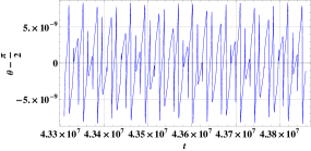
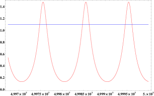
Figure 2: Plots of $\theta_{NO}(t)-\frac{\pi}{2}$ (left upper panel) and of $\theta_{Grav}(t)-\frac{\pi}{2}$ (right upper panel). In the bottom panels, $r_{Grav}-r_{NO}$ (left) and $t_{Grav}-t_{NO}$ (right) are plotted (red lines). The ratio between coordinated time $\frac{t_{Grav}}{\tau}$ versus proper time $\tau$ is also plotted (blue line). The examples we are showing have been obtained solving the system for the following parameters and initial conditions: $\mu=1.4M_{\odot}$, $r_{0}=500\mu$, $E=0.95$, $\phi_{0}=0$, $\theta_{0}=\frac{\pi}{2}$, $\dot{{\theta}_{0}}=0$, $\dot{\phi_{0}}=-\frac{1}{10}\dot{{r}_{0}}$ and $\dot{r}_{0}=-\frac{1}{100}$.

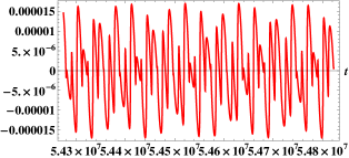
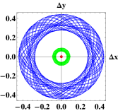
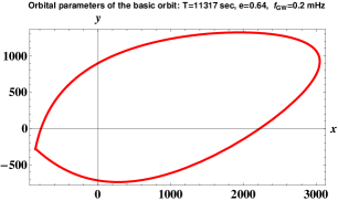
Figure 3: Plots of $z_{NO}(t)$ (left upper panel) and $z_{Grav}(t)$ (right upper panel). It is interesting to see the differences of about five orders of magnitude between the two plots. At the beginning, the effect is very small but, orbit by orbit, it grows and, for a suitable interval of coordinated time, the effect cannot be neglected (see the left bottom panel in which the differences in $x$ and $y$, starting from the initial orbits up to the last ones, by steps of about 1500 orbits, are reported). The internal red circle represents the beginning, the middle one is the intermediate situation (green) and the blue one is the final result of the correlation between $\Delta x$ versus $\Delta y$, being $\Delta x=x_{Grav}-x_{NO}$ and $\Delta y=y_{Grav}-y_{NO}$. On the bottom right, it is shown the basic orbit.

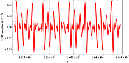
Figure 4: Plot of the differences of total gravitational waveform $h$, with and without the gravitomagnetic orbital correction for a neutron star of $1.4M_{\odot}$ orbiting around a MBH . The waveform has been computed at the Earth-distance from SgrA^∗ (the central Galactic Black Hole). The example we are showing has been obtained solving the systems for the following parameters and initial conditions: $\mu\approx 1.4M_{\odot}$, $r_{0}$, $E=0.95$, $\phi_{0}=0$, $\theta_{0}=\frac{\pi}{2}$, $\dot{\theta}_{0}=0$, $\dot{\phi_{0}}=-\frac{1}{10}\dot{r}_{0}$ and $\dot{r}_{0}=-\frac{1}{100}.$ It is worth noticing that frequency modulation gives cumulative effects after suitable long times.

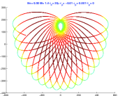
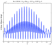
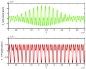
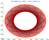
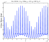
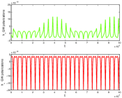
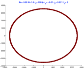
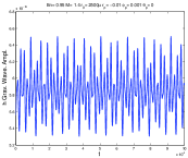
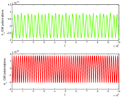
Figure 5: Plots along the panel lines from left to right of field velocities along the axes of maximum covariances, total gravitational emission waveform $h$ and gravitational waveform polarizations $h_{+}$ and $h_{\times}$ for a neutron star of $1.4M_{\odot}$. The waveform has been computed for the Earth-distance from Sagittarius A (the central Galactic Black Hole SgrA^∗). The plots we are showing have been obtained solving the system for the following parameters and initial conditions: $\mu\approx 1.4M_{\odot}$, $E=0.95$, $\phi_{0}=0$, $\theta_{0}=\frac{\pi}{2}$, $\dot{\theta_{0}}=0$, $\dot{\phi_{0}}=-\frac{1}{10}\dot{r}_{0}$ and $\dot{r}_{0}=-\frac{1}{100}$. From top to bottom of the panels, the orbital radius is $r_{0}=20\mu,\,1500\mu,\,2500\mu$. See also Table I.

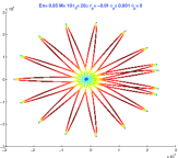
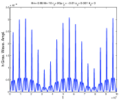
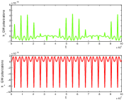
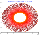
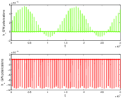
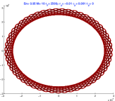
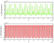
Figure 6: Plots along the panel lines from left to right of field velocities along the axes of maximum covariances, total gravitational emission waveform $h$ and gravitational waveform polarizations $h_{+}$ and $h_{\times}$ for a Black Hole (BH) of $10M_{\odot}$. The waveform has been computed for the Earth-distance to SgrA^∗. The plots we are showing have been obtained solving the system for the following parameters and initial conditions: $\mu\approx 10M_{\odot}$, $E=0.95$,$\phi_{0}=0$, $\theta_{0}=\frac{\pi}{2}$,$\dot{\theta_{0}}=0$,$\dot{\phi_{0}}=-\frac{1}{10}\dot{r}_{0}$ and $\dot{r}_{0}=-\frac{1}{100}$. From top to bottom of the panels, the orbital radius is $r_{0}=20\mu,\,1000\mu,\,2500\mu$. See also Table I

III Gravitational wave luminosity in the quadrupole approximation

After the discussion of gravitomagnetic corrections on the orbital motion, let us take into account the problem of how GW production and waveforms are affected by such effects. To this purpose, let us start with a short review of the quadrupole approximation for the gravitational radiation. This is, in our opinion, the best way to see how gravitomagnetic effects correct GW luminosity and waveforms.

It is well known that the Einstein field equations give a description of how the curvature of space-time is related to the energy-momentum distribution. In the weak field approximation, moving massive objects produce gravitational waves which propagate in the vacuum with the speed of light. In this approximation, we have

$$g_{\mu\nu}=\delta_{\mu\nu}+\kappa h_{\mu\nu},\qquad\left(\left|h_{\mu\nu}\right|<<1\right),$$ (12)

being $\kappa$ the gravitational coupling. The field equations are

$$\square\bar{h}_{\mu\nu}=-\frac{1}{2}\kappa T_{\mu\nu}$$ (13)

where

$$\bar{h}_{\mu\nu}=h_{\mu\nu}-\frac{1}{2}\delta_{\mu\nu}h_{\lambda\lambda}\,,$$ (14)

and $T_{\mu\nu}$ is the total stress-momentum-energy tensor of the source, including the gravitational stresses.

A plane GW, solution of (13), can be written as

$$\bar{h}_{\mu\nu}=h_{\mu\nu}=he_{\mu\nu}\cos(\omega t-\bm{\mathbf{k}\cdot\mathbf{x}})$$ (15)

where $h$ is the amplitude, $\omega$ the frequency, $k$ the wave number and $e_{\mu\nu}$ is a unit polarization tensor, obeying the conditions

$$e_{\mu\nu}=e_{\nu\mu},\qquad e_{\mu\mu}=0,\qquad e_{\mu\nu}e_{\mu\nu}=1.$$ (16)

Assuming a gauge in which $e_{\mu\nu}$ is space-like and transverse, a wave travelling in the z direction has two possible independent polarizations:

$$e_{1}=\frac{1}{\sqrt{2}}(\hat{x}\hat{x}-\hat{y}\hat{y})\qquad e_{2}=\frac{1}{\sqrt{2}}(\hat{x}\hat{y}-\hat{y}\hat{x}).$$ (17)

One can search for wave solutions of (13), generated by a system of masses undergoing arbitrary motions, and then obtain the radiated power. The result, assuming the source dimensions very small with respect to the wavelengths (i.e. the quadrupole approximation landau ), is that the power ${\displaystyle\frac{dE}{d\Omega}}$, radiated in a solid angle $\Omega$ with polarization $e_{ij}$, is

$$\frac{dE}{d\Omega}=\frac{G}{8\pi c^{5}}\left(\frac{d^{3}Q_{ij}}{dt^{3}}e_{ij}\right)^{2}$$ (18)

where $Q_{ij}$ is the quadrupole mass tensor

$$Q_{ij}=\sum_{a}m_{a}(3x_{a}^{i}x_{a}^{j}-\delta_{ij}r_{a}^{2})\leavevmode\nobreak\ ,$$ (19)

$r_{a}$ being the modulus of the vector radius of the $a-th$ particle and the sum running over all masses $m_{a}$ in the system. We must note that the result is independent of the kind of stresses present into dynamics. If one sums Eq.(18) over the two allowed polarizations, one obtains

$$\sum_{pol}\frac{dE}{d\Omega} = \frac{G}{8\pi c^{5}}\left[\frac{d^{3}Q_{ij}}{dt^{3}}\frac{d^{3}Q_{ij}}{dt^{3}}-2n_{i}\frac{d^{3}Q_{ij}}{dt^{3}}n_{k}\frac{d^{3}Q_{kj}}{dt^{3}}-\frac{1}{2}\left(\frac{d^{3}Q_{ii}}{dt^{3}}\right)^{2}\right.$$ (20)

$$\left.+\frac{1}{2}\left(n_{i}n_{j}\frac{d^{3}Q_{ij}}{dt^{3}}\right)^{2}+\frac{d^{3}Q_{ii}}{dt^{3}}n_{j}n_{k}\frac{d^{3}Q_{jk}}{dt^{3}}\right]\,,$$

where $\hat{n}$ is the unit vector in the radiation direction. The total radiation rate is obtained by integrating Eq.(20) over all emission directions; the result is

$$P=\frac{dE}{d\Omega}=\frac{G}{c^{5}}\left(\frac{d^{3}Q_{ij}}{dt^{3}}\frac{d^{3}Q_{ij}}{dt^{3}}-\frac{1}{3}\frac{d^{3}Q_{ii}}{dt^{3}}\frac{d^{3}Q_{jj}}{dt^{3}}\right)\,.$$ (21)

It is then possible to estimate the amount of energy emitted in the form of GWs from a system of massive interacting objects. In this case, the components of the quadrupole mass tensor are

$$\begin{array}[]{lll}Q_{xx}=\mu r^{2}(3\cos{{}^{2}\phi}\sin{{}^{2}\theta}-1)\leavevmode\nobreak\ ,\\ \\ Q_{yy}=\mu r^{2}(3\sin{{}^{2}\phi}\sin{{}^{2}\theta}-1)\leavevmode\nobreak\ ,\\ \\ Q_{zz}=\frac{1}{2}r^{2}\mu(3\cos 2\theta+1)\leavevmode\nobreak\ ,\\ \\ Q_{xz}=Q_{zx}=r^{2}\mu(\frac{3}{2}\cos\phi\sin 2\theta)\leavevmode\nobreak\ ,\\ \\ Q_{yz}=Q_{zy}=r^{2}\mu(\frac{3}{2}\sin 2\theta\sin\phi)\leavevmode\nobreak\ ,\\ \\ Q_{xy}=Q_{yx}=r^{2}\mu\left(\frac{3}{2}\sin^{2}\theta\sin 2\phi\right)\leavevmode\nobreak\ ,\end{array}$$ (22)

where the masses $m_{i}$ have polar coordinates $\{r_{i}\sin\theta\cos\phi,\;r_{i}\sin\theta\sin\phi,\>r_{i}\cos\theta\}$ and $\mu$ is the reduced mass. The origin of the motions is taken at the center of mass. Such components can be differentiated with respect to time as in Eq.(21). The gravitomagnetic corrections affect, essentially, these quantities and, consequently, the GW amplitude $h$ and the radiation rate $P$ as we will see below.

IV Gravitational wave amplitude with gravitomagnetic corrections

Direct signatures of gravitational radiation are given by GW-amplitudes and waveforms. In other words, the identification of a GW signal is strictly related to the accurate selection of the waveform shape by interferometers or any possible detection tool. Such an achievement could give information on the nature of the GW source, on the propagating medium, and, in principle, on the gravitational theory producing such a radiation Dela .

Considering the formulas of previous Section, the GW-amplitude can be evaluated by

$$h^{jk}(t,R)=\frac{2G}{Rc^{4}}\ddot{Q}^{jk}\leavevmode\nobreak\ ,$$ (23)

$R$ being the distance between the source and the observer and, due to the above polarizations, $\{j,k\}=1,2$.

From Eq.(23), it is straightforward to show that, for a binary system where $m\ll M$ and orbits have gravitomagnetic corrections, the Cartesian components of GW-amplitude are

$$h^{xx}=2\mu\left[\left(3\cos^{2}\phi\sin^{2}\theta-1\right)\dot{r}^{2}+6r\left(\dot{\theta}\cos^{2}\phi\sin 2\theta-\dot{\phi}\sin^{2}\theta\sin 2\phi\right)\dot{r}+\right.$$

$$+r\left(\left(3\cos^{2}\phi\sin^{2}\theta-1\right)\ddot{r}+3r\left(\dot{\theta}^{2}\cos 2\theta\cos^{2}\phi-\dot{\phi}\dot{\theta}\sin 2\theta\sin 2\phi\right.\right.$$

$$\left.\left.\left.-\sin\theta\left(\sin\theta\left(\dot{\phi}^{2}\cos 2\phi+\ddot{\phi}\cos\phi\sin\phi\right)-\ddot{\theta}\cos\theta\cos^{2}\phi\right)\right)\right)\right]$$ (24)

$$h^{yy}= 2\mu\left[\left(3\sin^{2}\theta\sin^{2}\phi-1\right)\dot{r}^{2}+6r\left(\dot{\phi}\sin 2\phi\sin^{2}\theta+\dot{\theta}\sin 2\theta\sin^{2}\phi\right)\dot{r}\right.+$$

$$+r\left(\left(3\sin^{2}\theta\sin^{2}\phi-1\right)\ddot{r}+3r\left(\dot{\theta}^{2}\cos 2\theta\sin^{2}\phi+\dot{\phi}\dot{\theta}\sin 2\theta\sin 2\phi+\right.\right.$$

$$+ \left.\left.\left.\sin\theta\left(\ddot{\theta}\cos\theta\sin^{2}\phi+\sin\theta\left(\dot{\phi}^{2}\cos 2\phi+\ddot{\phi}\cos\phi\sin\phi\right)\right)\right)\right)\right]$$ (25)

$$h^{xy}=h^{yx}= 3\mu\left[\cos 2\phi\sin\theta\left(4\dot{\theta}\dot{\phi}\cos\theta+\ddot{\phi}\sin\theta\right)r^{2}+2\dot{r}\left(2\dot{\phi}\cos 2\phi\sin^{2}\theta+\dot{\theta}\sin 2\theta\sin 2\phi\right)r+\right.$$

$$+ \left.\frac{1}{2}\sin 2\phi\left(2\ddot{r}\sin^{2}\theta+r(t)\left(2\dot{\theta}^{2}\cos 2\theta-4\dot{\phi}^{2}\sin^{2}\theta+\ddot{\theta}\sin 2\theta\right)\right)r+\dot{r}^{2}\sin^{(}\theta\sin 2\phi\right]$$ (26)

where we are assuming geometrized units. The above formulas have been obtained from Eqs.(9), (10), (11) The gravitomagnetic corrections give rise to signatures on the GW-amplitudes that, in the standard Newtonian orbital motion, are not present (see for example DeLaurentis ; nucita ). On the other hand, as discussed in the Introduction, such corrections cannot be discarded in peculiar situations as dense stellar clusters or in the vicinity of galaxy central regions.

Finally, the expected strain amplitude turns out to be $h\simeq(h_{xx}^{2}+h_{yy}^{2}+2h_{xy}^{2})^{1/2}$. In particular, considering a monochromatic GW, we have two independent degrees of freedom which, in the TT gauge, are $h_{+}=h_{xx}+h_{yy}$ and $h_{\times}=h_{xy}+h_{yx}$. We are going to evaluate these quantities and results are shown in Figs. 3, 4, 5, 6.

IV.1 Numerical results

Now we have all the ingredients to estimate the effects of gravitomagnetic corrections on the GW-radiation. Calculations have been performed in geometrized units in order to evaluate better the relative corrections in absence of gravitomagnetism. For the numerical simulations, we have assumed the fiducial systems constituted by a $m=1.4M_{\odot}$ neutron star or $m=10M_{\odot}$ massive stellar object orbiting around a MBH $M\simeq 3\times 10^{6}M_{\odot}$ as SgrA^∗. In the extreme mass-ratio limit, this means that we can consider ${\displaystyle\mu=\frac{mM}{m+M}}$ of about $\mu\approx 1.4M_{\odot}$ and $\mu\approx 10M_{\odot}$. The computations have been performed starting with orbital radii measured in the mass unit and scaling the distance according to the values shown in Table I. As it is possible to see in Table I, starting from $r_{0}=20\mu$ up to $2500\mu$, the orbital eccentricity ${\displaystyle\bm{e}=\frac{r_{max}-r_{min}}{r_{max}+r_{min}}}$ evolves towards a circular orbit. In Table I, the GW-frequencies, in $mHz$, as well as the $h$ amplitude strains and the two polarizations $h_{+}$ and $h_{\times}$ are shown. The values are the mean values of the GW $h$ amplitude strains ($h=\frac{h_{max}+h_{min}}{2}$) and the maxima of the polarization waves (see Figs. 5 and 6). In Fig. 7, the fiducial LISA sensitivity curve is shown LISA considering the confusion noise produced by White Dwarf binaries (blue curve). We show also the $h$ amplitudes (red diamond and green circles for $\mu\approx 1.4M_{\odot}$ and $\approx 10M_{\odot}$ respectively). It is worth noticing that, due to very high Signal to Noise Ratio, the binary systems which we are considering result extremely interesting, in terms of probability detection, for the LISA interferometer (see Fig. 7).

Table 1: GW-amplitudes and frequencies as function of eccentricity $e$, reduced mass $\mu$, orbital radius $r_{0}$ for the two cases of fiducial stellar objects $m\simeq 1.4M_{\odot}$ and $m\simeq 10M_{\odot}$ orbiting around a MBH of mass $M\simeq 3\times 10^{6}M_{\odot}$.

$1.4M_{\odot}$

$10M_{\odot}$

$\frac{r_{0}}{\mu}$ $e$ $f(mHz)$ $h$ $h_{+}$ $h_{\times}$ $20$ $0.91$ $7.7\cdot 10^{-2}$ $2.0\cdot 10^{-22}$ $5.1\cdot 10^{-23}$ $5.1\cdot 10^{-22}$ $200$ $0.79$ $1.1\cdot 10^{-1}$ $1.2\cdot 10^{-20}$ $2.2\cdot 10^{-21}$ $3.1\cdot 10^{-20}$ $500$ $0.64$ $1.4\cdot 10^{-1}$ $6.9\cdot 10^{-20}$ $8.7\cdot 10^{-21}$ $1.7\cdot 10^{-19}$ $1000$ $0.44$ $1.9\cdot 10^{-1}$ $2.6\cdot 10^{-19}$ $6.4\cdot 10^{-20}$ $6.4\cdot 10^{-19}$ $1500$ $0.28$ $2.3\cdot 10^{-1}$ $4.8\cdot 10^{-19}$ $3.6\cdot 10^{-20}$ $1.2\cdot 10^{-18}$ $2000$ $0.14$ $2.7\cdot 10^{-1}$ $5.9\cdot 10^{-19}$ $4.9\cdot 10^{-20}$ $1.3\cdot 10^{-18}$ $2500$ $0.01$ $3.1\cdot 10^{-1}$ $5.9\cdot 10^{-19}$ $1.7\cdot 10^{-20}$ $9.2\cdot 10^{-19}$

$e$ $f(mHz)$ $h$ $h_{+}$ $h_{\times}$ $0.98$ $3.2\cdot 10^{-2}$ $1.5\cdot 10^{-18}$ $1.6\cdot 10^{-19}$ $4.3\cdot 10^{-18}$ $0.87$ $9.2\cdot 10^{-2}$ $1.5\cdot 10^{-16}$ $2.5\cdot 10^{-18}$ $4.1\cdot 10^{-16}$ $0.71$ $1.4\cdot 10^{-1}$ $8.5\cdot 10^{-16}$ $7.0\cdot 10^{-18}$ $2.4\cdot 10^{-15}$ $0.49$ $1.9\cdot 10^{-1}$ $2.0\cdot 10^{-15}$ $1.6\cdot 10^{-17}$ $5.6\cdot 10^{-15}$ $0.32$ $2.3\cdot 10^{-1}$ $2.7\cdot 10^{-15}$ $2.5\cdot 10^{-17}$ $7.4\cdot 10^{-15}$ $0.19$ $2.6\cdot 10^{-1}$ $2.8\cdot 10^{-15}$ $3.3\cdot 10^{-17}$ $7.6\cdot 10^{-15}$ $0.08$ $2.9\cdot 10^{-1}$ $2.1\cdot 10^{-15}$ $4.0\cdot 10^{-17}$ $5.6\cdot 10^{-15}$

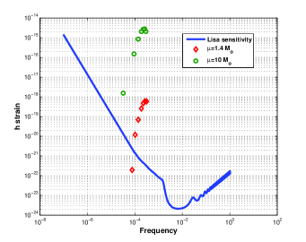
Figure 7: Plot of estimated mean values of GW-emission in terms of strain $h$ for two binary sources at the Galactic Center SgrA^∗ with reduced mass $\mu\approx 1.4M_{\odot}$ (red diamonds) and $\mu\approx 10M_{\odot}$(green circles). The blue line is the foreseen LISA sensitivity curve. The waveforms have been computed for the Earth-distance to SgrA^∗. The examples we are showing have been obtained solving the systems for the parameters and initial conditions reported in Figs. 5, 6 and in Table I.

V Event number estimations towards Sagittarius A^∗

At this point, it is important to give some estimates of the number of events where gravitomagnetic effects could be a signature for orbital motion and gravitational radiation. From the GW emission point of view, close orbital encounters, collisions and tidal interactions have to be dealt on average if we want to investigate the gravitational radiation in a dense stellar system. On the other hand, dense stellar regions are the favored target for LISA interferometer freitag so it is extremely useful to provide suitable numbers before its launching.

To this end, it is worth giving the stellar encounter rate producing GWs in astrophysical systems like dense globular clusters or the Galactic Center. In general, stars are approximated as point masses. However, in dense regions of stellar systems, a star can pass so close to another that they raise tidal forces which dissipate their relative orbital kinetic energy and the Newtonian mechanics or the weak field limit of GR cannot be adopted as good approximations. In some cases, the loss of energy can be so large that stars form binary (the situation which we have considered here) or multiple systems; in other cases, the stars collide and coalesce into a single star; finally stars can exchange gravitational interaction in non-returning encounters.

To investigate and parameterize all these effects, one has to compute the collision time $t_{coll}$, where $1/t_{coll}$ is the collision rate, that is, the average number of physical collisions that a given star suffers per unit time. As a rough approximation, one can restrict to stellar clusters in which all stars have the same mass $m$.

Let us consider an encounter with initial relative velocity $\mathbf{v}_{0}$ and impact parameter $b$. The angular momentum per unit mass of the reduced particle is $L=bv_{0}$. At the distance of closest approach, which we denote by $r_{coll}$, the radial velocity must be zero, and hence the angular momentum is $L=r_{coll}v_{max}$, where $v_{max}$ is the relative speed at $r_{coll}$. It is easy to show that binney

$$b^{2}=r_{coll}^{2}+\frac{4Gmr_{coll}}{v_{0}^{2}}\,.$$ (27)

If we set $r_{coll}$ equal to the sum of the radii of the two stars, a collision will occur if the impact parameter is less than the value of $b$, as determined by Eq.(27).

The function $f(\mathbf{v}_{a})d^{3}\mathbf{v}_{a}$ gives the number of stars per unit volume with velocities in the range $\mathbf{v}_{a}+d^{3}\mathbf{v}_{a}.$ The number of encounters per unit time with impact parameter less than $b$, which are suffered by a given star, is $f(\mathbf{v}_{a})d^{3}\mathbf{v}_{a}$ times the volume of the annulus with radius $b$ and length $v_{0}$, that is,

$$\int f(\mathbf{v}_{a})\pi b^{2}v_{0}d^{3}\mathbf{v}_{a}$$ (28)

where $v_{0}=\left|\mathbf{v-v}_{a}\right|$ and $\mathbf{v}$ is the velocity of the considered star. The quantity in Eq.(28) is equal to $1/t_{coll}$ for a star with velocity $\mathbf{v}$: to obtain the mean value of $1/t_{coll}$, we average over $\mathbf{v}$ by multiplying (28) by $f(\mathbf{v})/\nu$, where $\nu=\int f(\mathbf{v})d^{3}\mathbf{v}$ is the number density of stars and the integration is over $d^{3}\mathbf{v}$. Thus “

$$\frac{1}{t_{coll}}=\frac{\nu}{8\pi^{2}\sigma^{6}}\int e^{-(v^{2}+v_{a}^{2})/2\sigma^{2}}\left(r_{coll}\left|\mathbf{v-v}_{a}\right|+\frac{4Gmr_{coll}}{\left|\mathbf{v-v}_{a}\right|}\right)d^{3}\mathbf{v}d^{3}\mathbf{v}_{a}\,.$$ (29)

Replacing the variable $\mathbf{v}_{a}$ by $\mathbf{V}=\mathbf{v-v}_{a}$, the argument of the exponential is then $-\left[\left(\mathbf{v}-\frac{1}{2}\mathbf{V}\right)^{2}+\frac{1}{4}V^{2}\right]/\sigma^{2}$, and if we replace the variable $\mathbf{v}$ by ${\displaystyle\mathbf{v}_{cm}=\mathbf{v}-\frac{1}{2}\mathbf{V}}$ (the center of mass velocity), then one has

$$\frac{1}{t_{coll}}=\frac{\nu}{8\pi^{2}\sigma^{6}}\int e^{-(v_{cm}^{2}+V^{2})/2\sigma^{2}}\left(r_{coll}V+\frac{4Gmr_{coll}}{V}\right)dV\,.$$ (30)

The integral over $\mathbf{v}_{cm}$ is given by

$$\int e^{-v_{cm}^{2}/\sigma^{2}}d^{3}\mathbf{v}_{cm}=\pi^{3/2}\sigma^{3}\,.$$ (31)

Thus

$$\frac{1}{t_{coll}}=\frac{\pi^{1/2}\nu}{2\sigma^{3}}\int_{\infty}^{0}e^{-V^{2}/4\sigma^{2}}\left(r_{coll}^{2}V^{3}+4GmVr_{coll}\right)dV$$ (32)

The integrals can be easily calculated and then we find

$$\frac{1}{t_{coll}}=4\sqrt{\pi}\nu\sigma r_{coll}^{2}+\frac{4\sqrt{\pi}\nu Gmr_{coll}}{\sigma}\,.$$ (33)

The first term of this result can be derived from the kinetic theory. The rate of interaction is $\nu\Sigma\left\langle V\right\rangle$, where $\Sigma$ is the cross-section and $\left\langle V\right\rangle$ is the mean relative speed. Substituting $\Sigma=\pi r_{coll}^{2}$ and $\left\langle V\right\rangle=4\sigma/\sqrt{\pi}$ (which is appropriate for a Maxwellian distribution whit dispersion $\sigma$) we recover the first term of (33). The second term represents the enhancement in the collision rate by gravitational focusing, that is, the deflection of trajectories by the gravitational attraction of the two stars.

If $r_{*}$ is the stellar radius, we may set $r_{coll}=2r_{*}$. It is convenient to introduce the escape speed from stellar surface, ${\displaystyle v_{*}=\sqrt{\frac{2Gm}{r_{*}}}}$, and to rewrite Eq.(33) as

$$\Gamma=\frac{1}{t_{coll}}=16\sqrt{\pi}\nu\sigma r_{*}^{2}\left(1+\frac{v_{*}^{2}}{4\sigma^{2}}\right)=16\sqrt{\pi}\nu\sigma r_{*}^{2}(1+\Theta),$$ (34)

where

$$\Theta=\frac{v_{*}^{2}}{4\sigma^{2}}=\frac{Gm}{2\sigma^{2}r_{*}}$$ (35)

is the Safronov number binney . In evaluating the rate, we are considering only those encounters producing gravitational waves, for example, in the LISA range, i.e. between $10^{-4}$ and $10^{-1}$ Hz (see e.g. Rub ). Numerically, we have

$$\Gamma\simeq 5.5\times 10^{-10}\left(\frac{v}{10{\rm kms^{-1}}}\right)\left(\frac{\sigma}{UA^{2}}\right)\left(\frac{{\rm 10pc}}{R}\right)^{3}{\rm yrs^{-1}}\qquad\Theta<<1$$ (36)

$$\Gamma\simeq 5.5\times 10^{-10}\left(\frac{M}{10^{5}{\rm M_{\odot}}}\right)^{2}\left(\frac{v}{10{\rm kms^{-1}}}\right)\left(\frac{\sigma}{UA^{2}}\right)\left(\frac{{\rm 10pc}}{R}\right)^{3}{\rm yrs^{-1}}\qquad\Theta>>1$$ (37)

If $\Theta>>1$, the energy dissipated exceeds the relative kinetic energy of the colliding stars, and the stars coalesce into a single star. This new star may, in turn, collide and merge with other stars, thereby becoming very massive. As its mass increases, the collision time is shorten and then there may be runaway coalescence leading to the formation of a few supermassive objects per clusters. If $\Theta<<1$, much of the mass in the colliding stars may be liberated and forming new stars or a single supermassive objects (see Belgeman ; Shapiro ). Both cases are interesting for LISA purposes.

Note that when one has the effects of quasi-collisions (where gravitomagnetic effects, in principle, cannot be discarded) in an encounter of two stars in which the minimal separation is several stellar radii, violent tides will raise on the surface of each star. The energy that excites the tides comes from the relative kinetic energy of the stars. This effect is important for $\Theta>>1$ since the loss of small amount of kinetic energy may leave the two stars with negative total energy, that is, as a bounded binary system. Successive peri-center passages will dissipates more energy by GW radiation, until the binary orbit is nearly circular with a negligible or null GW radiation emission.

Let us apply these considerations to the Galactic Center which can be modelled as a system of several compact stellar clusters, some of them similar to very compact globular clusters with high emission in X-rays townes .

For a typical globular cluster around the Galactic Center, the expected event rate is of the order of $2\times 10^{-9}$ yrs^-1 which may be increased at least by a factor $\simeq 100$ if one considers the number of globular clusters in the whole Galaxy. If the stellar cluster at the Galactic Center is taken into account and assuming the total mass $M\simeq 3\times 10^{6}$ M_⊙, the velocity dispersion $\sigma\simeq$ 150 km s^-1 and the radius of the object $R\simeq$ 10 pc (where $\Theta=4.3$), one expects to have $\simeq 10^{-5}$ open orbit encounters per year. On the other hand, if a cluster with total mass $M\simeq 10^{6}$ M_⊙, $\sigma\simeq$ 150 km s^-1 and $R\simeq$ 0.1 pc is considered, an event rate number of the order of unity per year is obtained. These values could be realistically achieved by data coming from the forthcoming space interferometer LISA. As a secondary effect, the above wave-forms could constitute the ”signature” to classify the different stellar encounters thanks to the differences of the shapes (see Figs. 5 and 6).

VI Conclusions

In this paper we have discussed gravitomagnetic effects on orbital that could give rise to interesting phenomena in tight binding systems such as binaries of evolved objects (neutron stars or black holes). The effects become particularly relevant when such objects orbit around or fall toward very MBHs as those at the center of galaxies. The effects reveal particularly interesting if $v/c$ is in the range $(10^{-1}\div 10^{-4})c$. Gravitomagnetic orbital corrections, after long integration time, induce precession and nutation effects capable of affecting the stability basin of the orbits. The global structure of such a basin is extremely sensitive to the initial radial velocities and angular velocities, the initial energy and masses which can determine possible transitions to chaotic behavior. In principle, GW emission could present signatures of gravitomagnetic corrections after suitable integration times in particular for the on-going LISA space laser interferometric GW antenna.

References

- (1) A. Abramovici et al., Science 256 (1992) 325; http://www.ligo.org
- (2) B. Caron et al., Class. Quant. Grav. 14 (1997) 1461; http://www.virgo.infn.it
- (3) H. Luck et al., Class. Quant. Grav. 14 (1997) 1471; http://www.geo600.uni-hannover.de
- (4) M. Ando et al., Phys. Rev. Lett. 86 (2001) 3950; http://tamago.mtk.nao.ac.jp
- (5) http://www.lisa-science.org
- (6) E. Poisson, Living Rev. Rel. 6 (2004) 3, and references therein. http://relativity.livingreviews.org
- (7) Y.Mino, Prog. Theor. Phys. 113 (2005) 733; ibid. Prog. Theor. Phys. 115 (2006) 43; A. Pound, E. Poisson, and B.G. Nickel, Phys. Rev. D 72 (2005) 124001; L. Barack and C. Lousto, Phys. Rev. D 72 (2005) 104026; L. Barack and N. Sago, Phys. Rev. D 75 (2007) 064021.
- (8) L. S. Finn and K. S. Thorne, Phys. Rev. D 62 (2000) 124021; S. Babak et al. Phys. Rev. D 75 (2007) 024005; G. Sigl, J. Schnittman, and A. Buonanno, Phys. Rev. D 75 (2007) 024034.
- (9) R.D. Viollier Prog. Part. Nucl. Phys. 32 (1994) 51.
- (10) S. Capozziello, G. Iovane, Phys. Lett. A 259 (1999) 185.
- (11) S. Sigurdsson and M. Rees, Mont. Not. R. Astron. Soc., 284 (1997) 318.
- (12) S. Sigurdsson, Class. Quant. Grav. 14 (1997) 1425.
- (13) K. Danzmann et al., LISA- Laser Interferometer Space Antenna, Pre-Phase A Report, Max-Planck-Institut fur Quantenoptic,Report MPQ 233 (1998).
- (14) P. Amaro-Seoane et al., Class. Quant. Grav. 24 (2007) R113.
- (15) S. Capozziello, M. De Laurentis, F. Garufi and L. Milano, Phys. Scr. 79 (2009) 025901.
- (16) J.Binney and S.Tremaine, Galactic Dynamics, Princeton University Press, Princeton, New Jersey (1987).
- (17) L. Landau and E.M. Lifsits, Mechanics, Pergamon Press, New York (1973).
- (18) H. Thirring, Phys. Z. 19 (1918) 204
- (19) H. Thirring, Phys. Z., 19, (1918) 33; 22, (1921) 29; J. Lense and H. Thirring, Phys. Z., 19, (1918) 156. The english translation can be found in B. Mashhoon, F.W. Hehl and D.S. Theiss, Gen. Rel. Grav., 16, (1984) 711.
- (20) L. Iorio and V. Lainey, Int. Jou. Mod. Phys. D 14 (2005) 2039.
- (21) F. D. Ryan, Phys. Rev. D 56 (1997) 1845.
- (22) S. Capozziello and M. De Laurentis, Astrop. Phys. 30 (2008) 105.
- (23) S. Capozziello, M. De Laurentis, F. De Paolis, G. Ingrosso and A. Nucita, Mod. Phys. Lett. A 23(2008) 99.
- (24) L. Barack and C. Cutler, Phys. Rev. D 69 (2004) 082005.
- (25) L. Barack and C. Cutler, Phys. Rev. D 70 (2004) 122002.
- (26) M. Freitag, Astro. J. 583 (2003) L21.
- (27) S. Capozziello, M. De Laurentis, M. Francaviglia, Astrop. Phys. 29 (2008) 125.
- (28) L.J. Rubbo, K. Holley - Bockelmann, and L.S. Finn, Ap.J. 649 (2006) L25.
- (29) M.C. Belgeman and M.J. Rees Mon. Not. Roy. Astron. Soc., 185 (1978) 847.
- (30) A.P. Lightman and S. L. Shapiro Rev. Mod. Phys., 50 (1978) 437.
- (31) R. Genzel and C.H. Townes, Ann. Rev. Astron. Astroph. 25 (1987) 1.