The tunneling conductance between a superconducting STM tip and an out-of-equilibrium carbon nanotube

Abstract

We calculate the current and differential conductance for the junction between a superconducting (SC) STM tip and a Luttinger liquid (LL). For an infinite single-channel LL, the SC coherence peaks are preserved in the tunneling conductance for interactions weaker than a critical value, while for strong interactions ($g<0.38$), they disappear and are replaced by cusp-like features. For a finite-size wire in contact with non-interacting leads, we find however that the peaks are restored even for extremely strong interactions. In the presence of a source-drain voltage the peaks/cusps split, and the split is equal to the voltage. At zero temperature, even very strong interactions do not smear the two peaks into a broader one; this implies that the recent experiments of Y.-F. Chen et. al. (Phys. Rev. Lett. 102, 036804 (2009)) do not rule out the existence of strong interactions in carbon nanotubes.

Scanning tunneling spectroscopy (STM) is becoming an important tool for accessing the electronic properties of low-dimensional systems. Thus, in the past, the local density of states (DOS) for various materials such as the cuprates [1], graphene [2], and carbon nanotubes[3] has been studied, both theoretically and experimentally. In general the STM tip is assumed to be a non-interacting metal with a constant DOS, and the system to be analyzed is in equilibrium (the voltage is constant throughout the sample). This allows one to extract the unknown DOS directly from the STM tunneling conductance.

Recently a few studies have also concentrated on tips that are not normal metals, and that may have an intrinsic variation in the DOS, such as superconducting (SC) STM tips [4, 5]. These experiments have the potential of measuring not only the DOS, but also other quantities such as the Fermi distribution. The first such experiment [4] looked at a non-interacting system, and found that in equilibrium the differential conductance from a SC STM tip shows the characteristic SC gap and coherence peaks, while in the presence of a voltage bias each peak splits into two peaks, with the distance between them being given by the applied voltage. For a non-interacting system this splitting can be traced back to an out-of-equilibrium double-step Fermi distribution.

Similar experiments have been performed recently on carbon nanotubes [5], but the interpretation of these measurements is not so straightforward, due to the presence of strong electronic interactions which make the elementary excitations no longer fermionic but rather fractionally-charged. One might naively expect that the Fermi distribution is ill-defined in these systems, and that the strong electronic interactions contribute to the smearing of the two SC coherence peaks into a single one. On the other hand the experiments of [5] show the presence of two coherence peaks, which, when combined with this naive expectation, appear to imply that the interactions in nanotubes are weak !

To fully assess the implications of this experiment, and to test whether the expectation that the peaks merge is borne out of rigorous calculations, one needs to study theoretically the injection of electrons into a strongly-interacting out-of-equilibrium one-dimensional system. This is rather a challenging problem, that has not begun to be addressed theoretically until quite recently [6, 7, 8, 9].

We study the injection from a SC tip into an out-of-equilibrium LL, and we show that, even in the presence of very strong interactions, the tunneling conductance is very similar to that of a non-interacting wire. Our calculations therefore demonstrate that the apparently non-interacting features observed in [5] do not rule out the existence of strong interactions in carbon nanotubes.

We begin by analyzing an infinite single-channel LL wire in equilibrium, and we find that the tunneling conductance displays SC coherence peaks for interactions weaker than a critical value, corresponding to a fractional charge parameter, $g$, larger than $g_{c}=0.38$. Beyond this value the coherence peaks disappear, and are replaced by cusp-like features. Upon taking into account the finite size of the wire [10, 11, 12] and the presence of non-interacting contacts (as in the experiment of [5]) we find that the peaks reappear for any value of $g$. Furthermore, the tunneling conductance shows also oscillations with a period inverse proportional to the length of the wire and has a background power-law dependence whose exponent depends on the strength of the interactions.

If a voltage is applied between the ends of the wire, the peak/cusp features split. The magnitude of the split is exactly equal to the applied voltage. At zero temperature we never see a smearing of the two peaks into a single one, regardless of the strength of the interaction. Hence, the expectation that interactions cause the two peaks to merge into one is not correct. This in turn implies that the presence of two peaks found in [5] can not be used to rule out the presence of strong interactions in nanotubes !

Our calculations show that the experimental setup of [5] can be used to asses the strength of the interactions if one focuses instead on the power-law dependence of the density of states. If one measured the density of states for a wide-enough range of voltages (up to tens of meV) the data should allow to extract the value of the interaction parameter $g$.

A quantum wire connected to metallic leads is described by the Hamiltonian

$${\mathcal{H}}={\mathcal{H}}_{0}\,+\,{\mathcal{H}}_{V}\;.$$ (1)

Here ${\mathcal{H}}_{0}$ describes the interacting wire and the leads in the framework of the inhomogeneous single-channel LL model [10, 11, 12, 7] (we will discuss at the end how our results are affected by the presence of the extra channels of conduction in nanotubes). Explicitly:

$${\mathcal{H}}_{0} = \frac{\hbar v_{F}}{2}\int_{-\infty}^{\infty}dx\left[\Pi^{2}+\frac{1}{g^{2}(x)}(\partial_{x}\Phi)^{2}\right]$$ (2)

$${\mathcal{H}}_{V} = -\int_{-\infty}^{\infty}\frac{dx}{\sqrt{\pi}}\,\mu(x)\,\partial_{x}\Phi(x,t)\;,$$ (3)

where ${\mathcal{H}}_{V}$ describes the chemical potential applied to the wire. The interaction parameter $g(x)$ is space-dependent and its value is $g$ in the bulk of the wire, and 1 in the leads. For convenience, the end-points of the wire are denoted by $x_{1}=-L/2$ and $x_{2}=L/2$. The chemical potential is chosen such that $\mu(x)=-V_{SD}/2$ for $x<-L/2$ (left lead), $\mu(x)=V_{SD}/2$ for $x>L/2$ (right lead), and $\mu(x)=0$ for $-L/2<x<L/2$

Tunneling is allowed between the wire and a superconducting tip at at $x=0$. A schematic view of the system is shown in Fig. 3. The voltage of the tip is fixed at $V$.

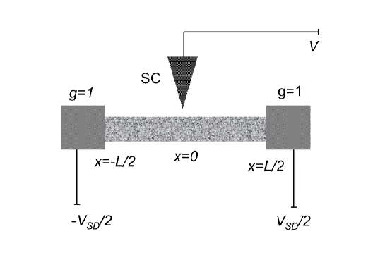
Figure 1: A quantum wire adiabatically coupled to metallic leads. The leads are held at different chemical potentials $\mu_{1}=-eV_{SD}/2$ and $\mu_{2}=eV_{SD}/2$. The electrons can tunnel from and into a superconducting STM tip at $x=0$. The voltage of the tip is fixed at $V$.

The Hamiltonian for the SC tip is assumed to be of the BCS type with a linear dispersion ($\epsilon_{k}\propto k$) and with a SC BCS coupling,

$$H_{tip}=\sum_{k}\sum_{\alpha=\uparrow,\downarrow}\epsilon_{k}c^{\dagger}_{k\alpha}c_{k\alpha}+(\Delta c_{k\uparrow}c_{-k\downarrow}+h.c.).$$ (4)

Our results do not depend on the details of the dispersion and of the dimensionality of the tip, as long as the tip DOS has the standard BCS form $\nu_{t}(\epsilon)=\theta(\epsilon-\Delta)\epsilon/\sqrt{\epsilon^{2}-\Delta^{2}}$.

The tunneling between the tip and the wire is described by the local Hamiltonian

$$H_{T}=tc^{\dagger}_{\alpha}(x=0)[\Psi^{R}_{\alpha}(x=0)+\Psi^{L}_{\alpha}(x=0)]+h.c$$ (5)

where $\Psi^{R/L}_{\alpha}(x)$ are the chiral fermionic interacting operators that can be related to the free bosonic modes of the LL via bosonization [13].

We use the non-equilibrium Keldysh formalism and we perform a perturbative expansion up to second order in the tunneling coefficient $t$, using the formalism developed in Ref. [7] to calculate the tunneling current between a normal tip and an out-of-equilibrium LL. We find that the tunneling current between the SC tip and the wire at zero temperature is

$$I\propto|t|^{2}\int_{0}^{\infty}dtQ_{T}(t){\rm Im}\{\exp[{\cal R}(t)+i{\cal I}(t)]{\cal F}_{s}(t)\}\,,$$ (6)

where for a finite-size wire [7]

$$Q_{T}(t)=2\cos\left(\frac{V_{SD}t}{2}\right)\sin(Vt)\,,$$ (7)

and

$$\mathcal{R}(t) = -\frac{1}{32\pi}\left\{\left(g+g^{-1}-2\right)\sum_{m\in Z_{\rm even}}\rho^{|m|}\ln{\frac{\alpha_{W}^{2}+(\tau+m)^{2}}{\alpha_{W}^{2}+m^{2}}}\right.$$ (10)

$$+\left(g+g^{-1}+2\right)\sum_{m\in Z_{\rm even}}\rho^{|m|}\ln{\frac{\alpha_{W}^{2}+(\tau-m)^{2}}{\alpha_{W}^{2}+m^{2}}}$$

$$+\left(g-g^{-1}\right)\sum_{m\in Z_{\rm odd}}\rho^{|m|}\left(\ln{\frac{\alpha_{W}^{2}+(\tau+m)^{2}}{\alpha_{W}^{2}+m^{2}}}+\ln{\frac{\alpha_{W}^{2}+(\tau-m)^{2}}{\alpha_{W}^{2}+m^{2}}}\right)\}$$

$$\mathcal{I}(t) = -\frac{1}{16\pi}\left\{\left(g+g^{-1}-2\right)\sum_{m\in Z_{\rm even}}\rho^{|m|}\arctan{\left(\frac{\tau+m}{\alpha_{W}}\right)}\right.$$ (13)

$$+\left(g+g^{-1}+2\right)\sum_{m\in Z_{\rm even}}\rho^{|m|}\arctan{\left(\frac{\tau-m}{\alpha_{W}}\right)}$$

$$\left.+\left(g-g^{-1}\right)\sum_{m\in Z_{\rm odd}}\rho^{|m|}\left[\arctan{\left(\frac{\tau+m}{\alpha_{W}}\right)}+\arctan{\left(\frac{\tau-m}{\alpha_{W}}\right)}\right]\right\}\,,$$

with $\tau\equiv tv_{F}/gL$, $\rho\equiv(1-g)/(1+g)$, and $\alpha_{W}$ is a dimensionless short-length cutoff. The quantity $Q_{T}(t)$ incorporates the effects of the applied tip voltage and source-drain voltage, while $\mathcal{R}(t)$ and $\mathcal{I}(t)$ are related to the Green’s functions of the system and incorporate information about the finite size via $\tau$. For an infinite wire one should substitute these quantities by:

$$\mathcal{R}(t)=-\frac{1}{16\pi}\left(g+g^{-1}\right)\ln{\frac{a_{W}^{2}+t^{2}}{a_{W}^{2}}}$$ (14)

$$\mathcal{I}(t)=-\frac{1}{8\pi}\left(g+g^{-1}-2\right)\arctan{\left(\frac{t}{a_{W}}\right)}\,.$$ (15)

Here $a_{W}$ is a short-time (high-energy) cutoff for the infinite wire.

For the superconducting tip, by taking a Fourier transform of the usual SC Green’s function we obtain

$${\cal F}_{s}(t)=\Delta K_{1}[(it+a_{T})\Delta]\,,$$ (16)

where $a_{T}$ is a short-time (high-energy) cutoff for the tip, and $K_{1}$ is the first Bessel $K$ function.

For a finite wire we can use the formulae above to compute the differential conductance $dI/dV$ numerically. For an infinite wire this calculation can be performed analytically, by rewriting (along the lines of [8]) the derivative of the tunneling current as:

$$\frac{dI}{dV}\propto\sum_{\eta=\pm 1}|t|^{2}\int_{0}^{\infty}d\epsilon\frac{d\nu_{t}(\epsilon)}{d\epsilon}(|\epsilon+V+\eta V_{SD}/2|^{\gamma}-|\epsilon-V-\eta V_{SD}/2|^{\gamma})$$ (17)

where $\gamma\equiv(g+1/g-2)/2$ and $\nu_{t}(\epsilon)$ is the density of states of the superconducting tip. This integral now gives:

$$\frac{dI}{dV}\propto i\sum_{\eta=\pm 1}|t|^{2}[|\Delta-V-\eta V_{SD}/2|^{\gamma-1/2}{{}_{2}F_{1}}(3/2,-1/2;3/2-\gamma;\Delta/2+V/2+\eta V_{SD}/4)+$$ (18)

$$|\Delta+V+\eta V_{SD}/2|^{\gamma-1/2}{{}_{2}F_{1}}(3/2,-1/2;3/2-\gamma;\Delta/2-V/2-\eta V_{SD}/2)]$$

where ${}_{2}F_{1}$ is the corresponding hypergeometric function.

We expand this function (in equilibrium – $V_{SD}=0$) close to the singularity at $V=\Delta$ and at $V\gg\Delta$. When $V\approx\Delta$:

$$\frac{dI}{dV}\propto(V-\Delta)^{\gamma-1/2}\,.$$ (19)

For non-interacting systems $\gamma=0$, and the tunneling conductance diverges as expected: $\frac{dI}{dV}\propto(V-\Delta)^{-1/2}$. In the presence of interactions this exponent is modified. For very strong interactions $\gamma$ increases, the exponent changes sign, and the divergence is replaced by a power-law-type cusp. This regime is achieved when $\gamma>1/2$, which corresponds to $g<0.38$.

When $V\gg\Delta$ we obtain

$$\frac{dI}{dV}\propto V^{\gamma}\,.$$ (20)

For non-interacting systems the tunneling conductance is constant at large V. In the presence of interactions the conductance acquires a power-law background with a positive exponent $\gamma$ as expected for tunneling into a LL.

In Figs. 2 a) and b) we plot the tunneling conductance for $V_{SD}=0$, for $g=1$ and $g=0.5$. We take $\Delta=1$ in arbitrary units. In Figs. 2 c) and d) we plot the corresponding tunneling conductance when $V_{SD}=\Delta$. As described above, for $g=0.5>g_{c}$ the SC coherence peaks are preserved in the spectrum. When the wire is out of equilibrium, Eq. (18) implies that the tunneling conductance is given by the sum of two tunneling conductances, which are shifted respectively by $\pm V_{SD}/2$.

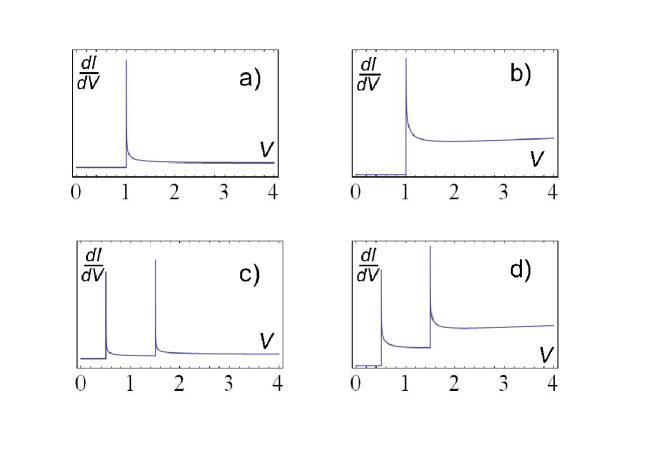
Figure 2: The tunneling conductance from an STM tip into an infinite Luttinger liquid (in arbitrary units) for LL interaction parameters $g=1$ (in a) and c)) and $g=0.5$ (in b) and d)). The source-drain voltage $V_{SD}$ is zero for a) and b), and is $V_{SD}=\Delta=1$ for c) and d).

In Figs. 3 a) and c) we repeat the same calculation for $g=0.3<g_{c}$. We see that indeed the peaks disappear and are replaced by cusp-like features, corresponding to a power-law decay of the tunneling conductance (19).

Our results change significantly if we take into account the finite size of the wire and the presence of metallic contacts. The integrals can now only be done numerically. In Fig. 3 b) and d) we plot the tunneling conductance for $g=0.3$ for a finite-size wire with characteristic finite-size energy scale $\omega_{L}=\hbar v_{F}/gL=\Delta/3$. We see that the peaks that disappear at infinite lengths are restored for a finite-size system. This is consistent with previous observations for nanotubes [10, 11, 12]: when $V-\Delta\ll\omega_{L}$ the physics is dominated by long wavelengths and is hence non-interacting.

Most importantly, for both infinite and finite systems, the two features at $\Delta\pm V_{SD}/2$ are not smeared into a single one, regardless of the strength of the interactions. Thus, as far as the peaks are concerned, even a very strongly interacting wire behaves as non-interacting. This is consistent with previous observations of a double-step out-of-equilibrium Fermi distribution [8], and explains why the features observed in Ref.[5] appear for both interacting and non-interacting systems. The only signatures of interactions are the disappearance of the peaks at very small $g$ for the infinite wire, and the power-law dependance of the tunneling conductance.

We should note that for a nanotube the parameter $\gamma$ is reduced from $(g+1/g-2)/2$ to $(g+1/g-2)/8$ because of the extra three channels of conduction [14]. Hence, the critical value of $g$ below which the peaks disappear is $g_{\rm cn}\approx 0.17$. Nevertheless, the finite-size effects are always relevant for non-chiral LLs, and hence we expect that the spectra presented in Figs. 3 b) and d), characterized by oscillations and SC coherence peaks, should describe the tunneling conductance between a SC tip and a nanotube in all situations.

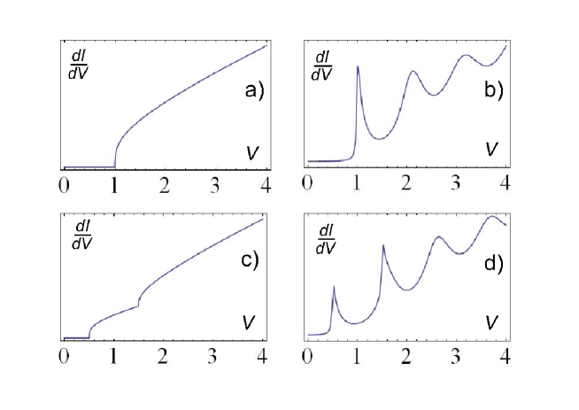
Figure 3: The tunneling conductance from a SC STM tip into an infinite (a) and c)) and finite-sized (b) and d)) $g=0.3$ Luttinger liquid. The source-drain potential $V_{SD}$ is zero for a) and b) and is $V_{SD}=\Delta=1$ for c) and d). The energy corresponding to the finite size of the wire, $\hbar v_{F}/gL$, is taken to be $\Delta/3$.

For a physical set of parameters, $\Delta=V=1.5meV$ and $\hbar v_{F}/gL\approx 0.5meV$ (corresponding to a tube length of $\approx 4\mu m$ at $g=0.25$), our results for the tunneling conductance reproduce very well those measured in [5] (compare for example Figs. 3 b) and 3 d) here with Figs. 2 c) and 3 in [5]).

To summarize, we have calculated the dependence on voltage of the STM tunneling conductance between a superconducting STM tip and an out-of-equilibrium Luttinger liquid. We have found that for an infinite single-channel LL in equilibrium, one can observe SC coherence peaks for interactions weaker than a critical value ($g<0.38$). Beyond this value, the coherence peaks disappear and are replaced by cusp-like features. We have also found that the peaks are restored if one takes into account the finite size of the LL and the presence of non-interacting contacts. For both infinite and finite-sized wires, the tunneling conductance shows a background power-law dependence, with an exponent that can be used to determine the strength of the interactions.

In the presence of an applied voltage between the ends of the wire, the tunneling-conductance features (peaks or cusps) split in two, and the magnitude of the split is equal to the voltage. Thus, there is no smearing of two peaks into a single one, regardless of the strength of interactions. This implies that the measurements of Ref.[5], that reveal features which appear naively to be non-interacting, do not in fact rule out the presence of strong interactions in carbon nanotubes.

Acknowledgments We would like to thank N. Mason, C. H. L. Quay, J. -D. Pillet, I. Safi and S. Vishveshwara for helpful discussions.

References

- [1] See e.g. K. McElroy, et. al., Science 309, 1048 (2005); M. Vershinin, et. al., Science 303, 1995 (2004); A. Fang et. al., Phys. Rev. B 70, 214514 (2004).
- [2] See e.g. P. Mallet et. al., Phys. Rev. Lett. 101, 206802 (2008); G. M. Rutter et. al.,Science 317 219 (2007); Y. Zhang, V. Brar, C. Girit, A. Zettl, M. F. Crommie, arXiv:0902.4793; G. Li, A. Luican, E. Y. Andrei, Phys. Rev. Lett 102, 176804 (2009).
- [3] B.J. LeRoy, S.G. Lemay, J. Kong, C. Dekker, Appl. Phys. Lett. 84, 4280 (2004); J. Lee, S. Eggert, H. Kim, S. J. Kahng, H. Shinohara, and Y. Kuk, Phys. Rev. Lett. 93, 166403 (2004); A. V. Lebedev, A. Crepieux, T. Martin, Phys. Rev. B 71, 075416 (2005); M. Guigou, T. Martin, and A. Crépieux, Phys. Rev. B 80, 045421 (2009) and Phys. Rev. B 80, 045420 (2009).
- [4] H. Pothier, S. Guéron, N. O. Birge, D. Esteve, and M. H. Devoret, Phys. Rev. Lett. 79, 3490 (1997).
- [5] Y.-F. Chen, T. Dirks, G. Al-Zoubi, N. O. Birge, and N. Mason, Phys. Rev. Lett. 102, 036804 (2009).
- [6] M. Trushin and A. L. Chudnovskiy, Europhys. Lett. 82 17008, 2008.
- [7] S. Pugnetti, F. Dolcini, D. Bercioux, and H. Grabert, Phys. Rev. B 79, 035121 (2009).
- [8] D. B. Gutman, Y. Gefen, and A. D. Mirlin, Phys. Rev. B 80, 045106 (2009).
- [9] I. Safi, arXiv:0906.2363.
- [10] I. Safi and H.J. Schulz, in Quantum Transport in Semiconductor Submicron Structures, NATO ASI, edited by B. Kramer (Kluwer, Dordrecht, 1995), Vol. 324, p. 159; I. Safi, Ann. Phys. (France) 22, 463 (1997); I. Safi, Eur. Phys. J. B 12, 451 (1999); I. Safi and H.J. Schulz, Phys. Rev. B 52, R17040 (1995).
- [11] D.L. Maslov and M. Stone, Phys. Rev. B 52, 5539 (1995); V.V. Ponomarenko, Phys. Rev. B 52, R8666 (1995); V.V. Ponomarenko and N. Nagaosa, Phys. Rev. B 60,16865 (1999); K.-I. Imura, K.-V. Pham, P. Lederer, F. Piechon, Phys. Rev. B 66, 035313 (2002).
- [12] F. Dolcini, H. Grabert, I. Safi, and B. Trauzettel, Phys. Rev. Lett. 91, 266402 (2003); B. Trauzettel, I. Safi, F. Dolcini, and H. Grabert, Phys. Rev. Lett. 92, 226405 (2004); F. Dolcini, B. Trauzettel, I. Safi, and H. Grabert, Phys. Rev. B 71, 165309 (2005).
- [13] M. P. A. Fisher and L. I. Glazman, Mes. Elec. Transp., ed. by L.L. Sohn, L.P. Kouwenhoven, and G. Schon, NATO Series E, Vol. 345, 331 (Kluwer Academic Publishing, Dordrecht, 1997).
- [14] C. L. Kane, L. Balents, and M. P. A. Fisher, Phys. Rev. Lett. 79, 5086 (1997); R. Egger and A.O. Gogolin, Phys. Rev. Lett. 79, 5082 (1997).