A constraint on brown dwarf formation via ejection: radial variation of the stellar and substellar mass function of the young open cluster IC 2391

Abstract

We present the stellar and substellar mass function of the open cluster IC 2391, plus its radial dependence, and use this to put constraints on the formation mechanism of brown dwarfs. Our multiband optical and infrared photometric survey with spectroscopic follow-up covers 11 square degrees, making it the largest survey of this cluster to date. We observe a radial variation in the mass function over the range 0.072 to 0.3 M_⊙, but no significant variation in the mass function below the substellar boundary at the three cluster radius intervals analyzed. This lack of radial variation for low masses is what we would expect with the ejection scenario for brown dwarf formation, although considering that IC 2391 has an age about three times older than its crossing time, we expect that brown dwarfs with a velocity greater than the escape velocity have already escaped the cluster. Alternatively, the variation in the mass function of the stellar objects could be an indication that they have undergone mass segregation via dynamical evolution. We also observe a significant variation across the cluster in the colour of the (background) field star locus in colour-magnitude diagrams and conclude that this is due to variable background extinction in the Galactic plane. From our preliminary spectroscopic follow-up to confirm brown dwarf status and cluster membership, we find that all candidates are M dwarfs (in either the field or the cluster), demonstrating the efficiency of our photometric selection method in avoiding contaminants (e.g. red giants). About half of our photometric candidates for which we have spectra are spectroscopically-confirmed as cluster members; two are new spectroscopically-confirmed brown dwarf members of IC 2391.

1 INTRODUCTION

The origin and evolution of brown dwarfs (BD) remains a fundamental open question. BDs have masses bridging the lowest mass hydrogen-burning stars and giant planets, so any picture of star and planet formation is incomplete if it cannot account for BDs. Several formation mechanisms have been proposed, including star-like formation from the compression and fragmentation of a dense molecular cloud, planet-like formation in a circumstellar disk, and the dynamical interruption of a star-like accretion process.

There are observational signatures which may be used to distinguish between these scenarios, such as the distribution of binaries, the presence and properties of circumstellar disks, the (initial) mass function (MF) and kinematics (see Luhman et al. 2007 for a review of observational signatures on the formation of BDs). Work over the past ten years has seen considerable success in measuring the MF into the BD regime in several clusters, including $\sigma$ Orionis (Gonsález-García et al. 2006; Caballero et al. 2007; Lodieu et al. 2009), the Orion Nebula Cluster (ONC) (Hillenbrand et al. 2000; Slesnick et al. 2004), IC 2391 (Barrado y Navascués et al. 2004; Platais et al. 2007) and the Pleiades (Moraux et al. 2003; Lodieu et al. 2007). These are only examples among many other analysis of stellar and substellar populations.

The comparison of the MF in clusters with different properties (e.g. the different density clusters Taurus and ONC; clusters with different ages, e.g. Chabrier 2003) has led some workers to draw conclusions about the relative efficiency of possible BD formation mechanisms (e.g. Kroupa & Bouvier 2003). While some observations (Luhman et al. 2007) and theoretical works (Padoan & Nordlund 2004; Hennebelle & Chabrier 2008) conclude in a common formation mechanism for BDs and stars, some studies has suggested that BDs could form by massive disc fragmentation (Stamatellos & Whitworth 2008), photoevaporation of the accretion envelope (Hester et al. 1996), or interruption of the accretion process (Reipurth 2000; Reipurth & Clarke 2001). For instance, Bate & Bonnell (2005) have performed hydrodynamical simulations of star formation from fragmentation of molecular clouds. They concluded that objects which end up as BDs stop accreting before they reach the hydrogen burning limit because they are ejected from the dense gas soon after their formation by dynamical interaction in unstable multiple systems.

This ejection scenario in some cases predicts a higher velocity dispersion and spatial spread of BDs in comparison to stellar objects, which in turn may be observed as a variation in the MF with radius (Kroupa & Bouvier 2003). On the other hand, other work have shown that if BDs are formed by ejection, the velocity distribution could be the same for BDs and stars (Bate 2009). Muench et al. (2003) observed a radial variation in the MF of IC 348 measured over 0.5 to 0.08 M_⊙, but no variation was detected in the BD regime. In a study of the spatial distribution of substellar objects in IC 348 as well as Trapezium in the Orion Nebula Cluster, Kumar & Schmeja (2007) observed the stellar objects to be more clustered than the substellar ones, which they took as evidence in favour of the ejection scenario. By looking at the spatial distribution of the Taurus stellar and substellar population, Guieu et al. (2006) observed a gradient in the BD abundance relative to stars, which they conclude as in favour of the ejection scenario.

In this paper, we present the results of a program to study, in detail, the MF of one of the nearest and richest open clusters, IC 2391. This has an age of 50 Myr measured from lithium depletion (Barrado y Navascués et al. 2004) or 40 Myr from main-sequence fitting (Platais et al. 2007). The Hipparcos distance is 146.0${}^{+4.8}_{-4.5}$ pc (Robichon et al. 1999) and the metalicity and extinction are [Fe/H]$=-0.03\pm 0.07$ and $E(B-V)=0.01$, (Randich et al. 2001). Because of its proximity and youth, this cluster has been subject to several studies (e.g. Barrado y Navascués et al. 2004, 2001, 1999; Koen & Ishihara 2006; Siegler et al. 2007; Platais et al. 2007). Barrado y Navascués et al. (2004) and Dodd (2004) measured the MF down to the substellar limit, but the MF for confirmed member with a completeness limit at lower masses has not yet been determined.

Since IC 2391 is not as young as IC 348 (age $\sim$ 2 Myr from Muench et al. 2003) and Trapezium (age $\sim$ 0.8 Myr from Muench et al. 2002), one may expect it has already lost a significant fraction of its substellar population to evaporation by dynamical evolution. Using the tidal radius and mass of IC 2391 estimated by Piskunov et al. (2007) (7.4 pc and 175 M_⊙), we compute the escape velocity as $v_{e}=$0.4 km/s and the crossing as time $t_{cross}=$17 Myr. (We stress that the crossing time is just an order-of-magnitude quantity, 2R/v, where we have adopted for R the tidal radius of 7.4 pc from Piskunov et al. 2007 and the velocity dispersion of $\sim$0.85 km/s from Platais et al. 2007). Assuming a minimum value for the number of cluster members as the objects reported by Dodd (2004) and Barrado y Navascués et al. (2004) (125 and 33 respectively, together a total lower limit of 158 objects), we estimate that the lower limit of the relaxation time for this cluster is $t_{relax}\sim$105 Myr. Furthermore, in a numerical simulation of open clusters and the population of BDs members, Adams et al. (2002) shows that there would still be more than 80% of the original BD population in the cluster even after about 10 crossing times, assuming that BDs and stars have a similar velocity dispersion. Therefore, IC 2391 is still young enough for a radial study of its very low mass star (VLMS) and BD populations, considering the fact that mass segregation occurs on a timescale of order one relaxation time (Bonnell & Davies 1998; although recent work by Allison et al. 2009 suggest that mass segregation can occur on a smaller time than a relaxation time, at least for more massive stars).

The paper is structured as follows. We will first present the data set, reduction procedure and calibration in §2. We then discuss our candidate selection procedure in §3, present the survey results in §4 and then discuss the radial variation of the MF in §5. The preliminary spectroscopic follow-up is presented in §6 followed by our conclusions in §7.

2 OBSERVATIONS, DATA REDUCTIONS AND CALIBRATIONS

2.1 Observations

The survey consists of 35 34$\times$33 arcmin fields extending to 3 degrees from the center of the cluster and centered on RA=08:40:36 DEC=-53:02:00 (Figure 1). The central 4 fields will be referred to as the deep fields while the other 31 other fields will be referred as the radial fields and outward fields. (We make a distinction since they were observed with different exposure times and different filters, as will be specified below). The fields were chosen to extend preferentially along lines of constant Galactic latitude in an attempt to reduce systematic errors in any established cluster MF gradient which could arise from contamination by a Galactic disk population gradient. The total coverage of our survey is 10.9 sq. deg. This compares to 2.5 deg² in the survey of Barrado y Navascués et al. (2001).

The optical observations were carried out in four runs with the Wide Field Image (WFI) on the 2.2m telescope at La Silla (Baade et al. 1999) in : 24 January - 9 February 1999, 20 - 24 January 2000, 10 - 23 March 2007 and 15 - 18 May 2007. The WFI is a mosaic camera comprising 4$\times$2 CCDs each with 2k$\times$4k pixels delivering a total field of view of 34$\times$33 arcmin at 0.238 arcsec per pixel. The deep fields in our survey were observed in four medium bands filters, namely 770/19, 815/20, 856/14 and 914/27 (where the filter name notation is central wavelength on the full width at half maximum, FWHM, in nm) and one broad band filter, $R_{\rm c}$. The radial fields were observed in $R_{\rm c}$, 815/20 and 914/27 while the five outward fields were not observed in $R_{\rm c}$.

These filters were chosen to sample the spectra of late M and early L dwarfs to improve selection over, say, $R_{\rm c}-I_{\rm c}$, and to minimize the Earth-sky background plus any nebular emission (as the filters are in regions of low emission). The pass band function for all filters are shown in Figure 2. For all radial fields, we have used an exposure time of 15, 10 and 25 minutes for the 815/20, 914/27 and $R_{\rm c}$ filters respectively. For each deep field we obtained an integration time of 65 minutes for each of 770/19 and $R_{\rm c}$ and from 50 to 155 minutes for 815/20, from 25 to 261 minutes for 856/14, and 50 to 80 minutes for 914/27. We additionally obtained short exposures for all fields to extend the dynamic range to brighter objects. The photometry from the short exposures were combined with the photometry of our long exposures for our analysis. In order to improve the determination of their low mass status (via a better determination of spectral type and luminosity), we also observed all radial fields, including the outward fields, in the $J$–band using the Caméra PAnoramique Proche-InfraRouge (CPAPIR) on the 1.5m telescope at Cerro Tololo, Chile (runs on 28 February - 3 March 2007 and 10 March 2007). However, we did not get $J$–band photometry for the deep fields. CPAPIR consists of one Hawaii II detector of 2k$\times$2k pixels for a field of view of 35$\times$35 arcmin with a pixel scale of 1.03 arcsec per pixel. All fields were observed with a total exposure time of 30 minutes. The $J$ filter of CPAPIR is centered at 1 250 nm with a FWHM of 160 nm. A detailed list of the fields observed with pointing, filter used, exposure time and 10$\sigma$ detection limit, is given in Table 1.

Our 10$\sigma$ detection limit is $J$=17.7 and $914/27$=20.5 for the radial and deep fields respectively (which corresponds to $\sim$0.03 M_⊙ for both cases). However, we can’t expect to detect all objects down to these magnitudes. The completeness spanning from the brightest objects without saturation down to the 10$\sigma$ detection limit is estimated by taking the ratio of the number of objects detected to the predicted number of detections and assuming a uniform distribution of stars along the line of sight in the fields of our survey. The predicted number of detections is derived very simply by extrapolating to the detection limit a linear fit to the histogram of the number of detections as a function of magnitude (Figure 3). The completeness of the radial part of the survey is 91.8% while for the deep part it is 82.7%.

The spectroscopic observations were carried out with HYDRA, a multi-object, fiber-fed spectrograph on the 4m telescope at Cerro Tololo on the nights of 6 and 7 January 2007. Only two fields could be observed: the deep fields 15 and 20 (3 and 2 exposures of 45 minutes respectively). We used the red fiber cable with the KPGLF grating (632 lines mm^-1) and a blaze angle of 14.7^∘ (no blocking filter was used) and . This gives us a coverage of 6429–8760 Å  centered at 7593 Å  and a spectral resolution of 4.0 Å.

2.2 Reduction and Astrometry

The standard CCD reduction steps (overscan subtraction, trimming and flat-fielding for the WFI data and dark subtraction, flat-fielding for CPAPIR data) were performed on a nightly basis using the $ccdred$ package under IRAF. For WFI data we used the dome flat both for pixel-to-pixel variation correction and to correct the global illumination, while for CPAPIR data we used superflat (obtained by combining science image frames for each nights). For WFI data, we reduced each of the 8 CCDs in the mosaic independently and in the final step scaled them to a common flux response level. We made an initial sky subtraction via a low-order fit to the optical data, and for the infrared data by subtracting a median combination of all (unregistered) images of the science frames. Images were fringe subtracted when fringes were visible, which was the case for all medium bands filters used, in a similar way as described by Bailer-Jones et al. (2001) Finally, the individual images of a given field were registered and median combined. We calculated magnitudes via aperture photometry together with an aperture correction following the technique used in Howell (1989). An astrometric solution was achieved using the IRAF package imcoords and the tasks ccxymatch, ccmap and cctran. For each field, this solution was computed for the 815/20 band image using the Two Micron All Sky Survey (2MASS) catalogue as a reference. The RMS accuracy of our astrometric solution is within 0.15–0.20 arcsec for WFI data and within 0.3–0.4 arcsec for CPAPIR data. For WFI data, the astrometry was also performed on a CCD-by-CCD basis.

We only retained images for this study which were taken under photometric conditions, as determined by our monitoring of conditions during the observations and, moreover, by our data reduction procedure.

2.3 Photometric Calibration

To correct for Earth-atmospheric absorption on the photometry, we solved by least squares fitting the equation,

$${m_{A}=m_{A,raw}+Z_{A}+C_{A}(m_{A}-m_{B})+\kappa_{A}X_{A}},$$ (1)

for observations of the standard stars at a range of airmasses, where the spectrophotometric standard stars observed were Hiltner 600, HR 3454 and LTT 3864. (In order to obtain the observed magnitude from equations 1, the fluxes of each standard star, $f_{\lambda}$, were taken from Hamuy et al. 1992, 1994.) The parameters $m_{A}$ and $m_{B}$ are the apparent magnitudes of our spectrophotometric standard in two particular bands ($A$ and $B$), where $m_{A,raw}$ is the instrumental magnitude of our spectrophotometric standard stars, $Z_{A}$ is the zero point offset, $C_{A}$ is the colour correction and $\kappa_{A}$ the extinction coefficient for band $A$ and $X$ is the airmass at which $m_{A,raw}$ was obtained.

We calibrated the infrared data using the $J$ band values of 2MASS objects which were observed in the science fields. By determining a constant offset between the magnitude of 2MASS and our instrumental magnitude, we obtained the zero point offset. Since this zero point offset was obtained with objects in the same field of view in each science frame, we did not perform a colour or airmass correction when reducing our NIR photometry.

2.4 Mass and Effective Temperature Based on Photometry

We used the spectral energy distribution to derive the mass and effective temperature, $T_{\rm eff}$, assuming that all our photometric candidates belong to IC 2391. We used evolutionary tracks from Baraffe et al. (1998) and atmosphere models from Hauschildt et al. (1999a) (assuming a dust-free atmosphere; the NextGen model) to compute an isochrone for IC 2391 using an age of 50 Myr, distance of 146 pc, a solar metalicity and neglecting the reddening ($E(B-V)$ = 0). These models and assumptions provide us with a prediction of $f_{\lambda}$, the spectral energy distribution received at the Earth (in erg cm^-2 s^-1 Å^-1) from the source. We need to convert these spectra to magnitudes in the filters we used. Denoting as $S_{A}$($\lambda$) the (known) total transmission function of filter $A$ (including the CCD quantum efficiency and assuming telescope and instrumental throughput is flat), then the flux measured in the filter is

$$f_{A}=\frac{\int_{0}^{\infty}f_{\lambda}S_{A}(\lambda)d\lambda}{\int_{0}^{\infty}S_{A}(\lambda)d\lambda},$$ (2)

The corresponding magnitude $m_{A}$ in the Johnson photometric system is given by

$${m_{A}=-2.5\;\mathrm{log}\;f_{A}\;+\;c_{A}},$$ (3)

where $c_{A}$ is a constant (zero point) that remains to be determined in order to put the model-predicted magnitude onto the Johnson system. We determine this constant for each of the bands $R_{\rm c}$, 770/19, 815/20, 856/14, 914/27 and $J$ in the standard way, namely by requiring that the spectrum of Vega produce a magnitude, $m_{A}$, of zero in all bands. Using the Vega spectrum from Colina et al. (1992) we derive values of $c_{Rc}=-21.6607$ $c_{770/19}=-22.2517$, $c_{815/20}=-22.4391$, $c_{856/14}=-22.6341$, $c_{914/27}=-22.8353$ and $c_{J}=-23.6865$ mag. Applying the two equations above to a whole set of model spectra produces a theoretical isochrone in colour–magnitude space. Note that this procedure only provides us with the “true” magnitudes of the model spectra, not their instrumental ones. The photometric calibration procedure applied to the data converts the measured, instrumental magnitudes to the “true” magnitude plane where we can compare them.

Assuming that all our photometric candidates belong to IC 2391, we derive masses and effective temperatures in the following way. We first normalize the measured spectral energy distribution (multiband photometry) of each object to the energy distribution of the model using the 815/20 filter. We then estimate the mass and effective temperature (which are not independent of course) via a least squares fit between the measured spectral energy distribution and the model spectral energy distribution from the isochrone.

There are several sources of error in the mass and $T_{\rm eff}$ estimates. These come from the photometry, the photometric calibration, the least squares fitting (imperfect model) and the uncertainties on the age of IC 2391 (we use 5 Myr). This last and most significant error gives 0.075$\pm$0.006 M_⊙ and 2914$\pm$43 K for an object at the hydrogen burning limit and 1.000$\pm$0.027 $M_{\odot}$ and 5270$\pm$70 K for a solar type object.

2.5 Spectroscopic Data Reduction and Calibration

The standard CCD reductions (overscan subtraction and trimming) were performed on each image using the $ccdred$ package under IRAF. We then used the IRAF package $dohydra$ to perform flat-fielding (using dome flats), throughput correction (with the skyflats) and scattered light corrections. The spectra were wavelength calibrated using the PENRAY comparison lamp with 2 sec exposure time. Sky subtraction was performed in a similar manner as fringe subtraction in photometry: a standard sky spectrum (shown at Figure 4) was obtained from the median of our sky spectra (more than 20 fibers were assigned for sky subtraction in each Hydra pointing) and scaled to optimize the sky subtraction for each science spectrum individually. However, this sometimes resulted in H$\alpha$ apparently being in absorption for some objects. We attribute this to H$\alpha$ emission from the background itself. This is spatially variable and so subtracting the sky spectrum (which includes H$\alpha$) sometimes results in a over-subtraction of this feature. We discuss this contamination problem and the danger of determining membership status based on H$\alpha$ in §6.1.

Finally, flux calibration was performed with the spectrophotometric standard Hiltner 600, which was observed three times a night, at three different airmass.

2.6 Spectral type, effective temperature and mass determination

For the objects for which spectra is available, we estimated in addition the spectral type using the PC3 index from Martín et al. (1999). The distinction between M–dwarf and background M-giants and M-supergiants was achieved using a CaH index (Jones 1973). We visually inspected all spectra in order to confirm the spectral type and luminosity class estimation. We estimated a spectroscopic $T_{\rm eff}$ from the spectral type using the temperature scale of Luhman (1999) for objects between M1V to M9V and of Martín et al. (1999) for objects from L0V and later. We then use our isochrone of IC 2391 to obtain the mass based on $T_{\rm eff}$.

3 CANDIDATE SELECTION PROCEDURE

The selection procedure discuss here concerns only our photometric data while the discussion of the selection of our spectroscopic candidates is done in §6. The candidate selection procedure is as follows (and explained in more detail in the remainder of this section). Candidates were first selected based on colour-magnitude diagrams (CMDs). A second selection was performed using colour-colour diagrams. Third, astrometry was used to remove objects with high proper motion. Finally, non-candidates were rejected based on a discrepancy between the observed magnitude in 815/20 and the magnitude in this band computed with the isochrone of IC 2391 and our estimation of $T_{\rm eff}$. To be a cluster member in this work an object has to satisfy all four of these steps.

3.1 First Candidate Selection: CMDs

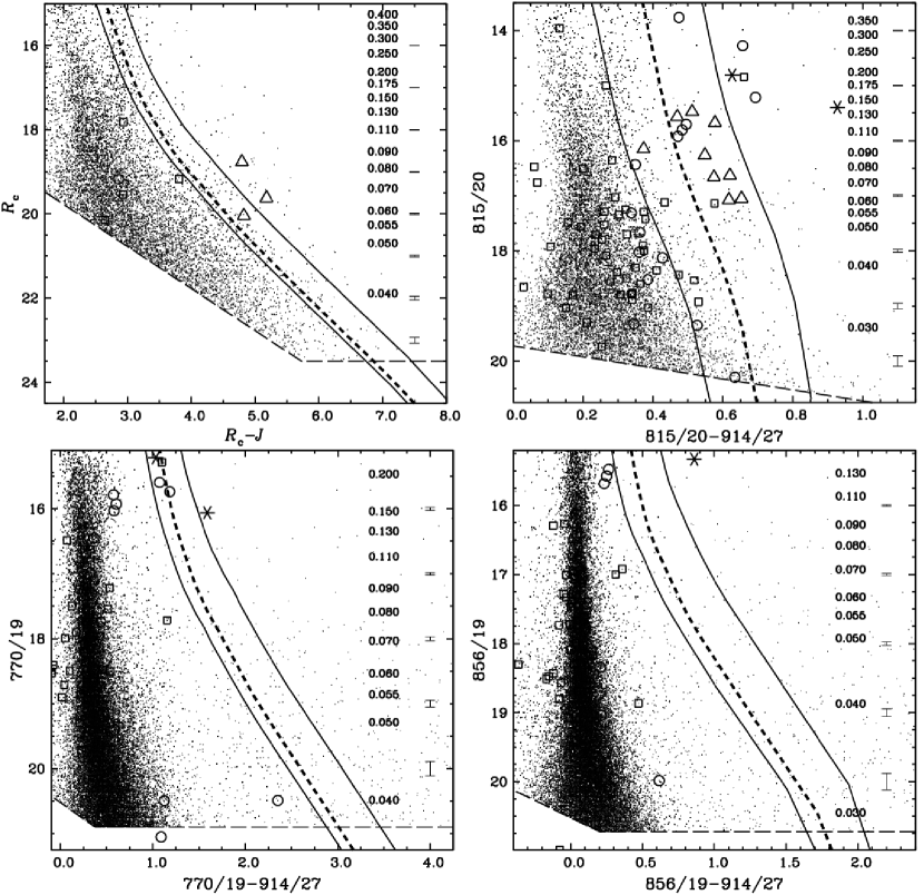
Figure 5: Top. Two CMDs from the radial field 01. As dotted lines we show the isochrone computed from an evolutionary model with a grainless atmosphere (NextGen model, the masses for each $R_{\rm c}$ are shown in the right panel). The thin dashed line is the 10$\sigma$ detection limit. We also show candidate low mass cluster members from Patten & Pavlovsky (1999) (stars), Barrado y Navascués et al. (2004) (triangles), Dodd (2004) (squares) and X-ray sources detected by XMM-Newton (circles), which we detected in our survey. Some of these objects are not present in the left panel since the deep fields, where most of these objects are detected, lack $J$-band photometry. Bottom. Two CMDs from the deep field 32 with medium bands. Isochrones, 10$\sigma$ detection limit and cluster members from previous studies are the same as for the top two panels. In each panel, the thin solid lines represent the selection curve and the errorbars present the photometric errors.

Candidates were first selected from our CMDs by keeping all objects which are no more than 0.15 mags redder or bluer than the isochrone in all CMDs (this number accommodates errors in the magnitudes and uncertainties in the model isochrone), plus errors from age estimation and distance to IC 2391 reflected on the isochrone. We additionally include objects brighter than 0.753 mag the isochrone in order to include unresolved binaries. In Figure 5 we show two CMDs for field 01 where candidates were selected based on 815/20 vs. 815/20–914/27 and $R_{\rm c}$ vs. $R_{\rm c}$–$J$ (top 2 panels). We also present two CMDs from the deep field 32 using the medium band 770/19, 856/14 and 914/27 (lower 2 panels). From a total of 20 008 114 objects detected, 174 511 are kept (99.2% are rejected).

We also present in this figure low mass cluster member candidates from previous work which we detected in our survey (Patten & Pavlovsky 1999, Barrado y Navascués et al. 2004, Dodd 2004 and X-ray sources detected by XMM-Newton where some are also presented in Marino et al. 2005). Some candidates from previous studies are simply not detected in our work. This is the case with Platais et al. (2007) where the faintest candidates have $V$$\sim$15, which corresponds to 0.6 M_⊙ (close to the saturation limit of the radial and outward fields at $\sim$0.9 M_⊙ and at the saturation limit of the central deep fields, also at $\sim$0.6 M_⊙). Also, no objects in our sample match the 34 members studied by Siegler et al. (2007) because either our images are too deep so bright stars saturate (e.g. HD74275, HD74374 and VXR22a, which saturate in the short exposures), or the objects are not in our fields (e.g. VXR06, SHJM10 and PP07, which are between fields 32 and 37). Also, no objects match within 4 arcsec between our objects and the 17 cluster candidates from Rolleston & Byrne (1997) for similar reasons: the bright stars saturate (e.g. object ID 162, 311 and 362, which are birghter then our saturation limit in $R_{\rm c}$), or the objects are not in our fields (e.g. object ID 729 and 955, which are in the central part of the cluster between fields 20 and 27).

Finally, we point out that the survey of IC 2391 based on proper motion done by Dodd (2004) only covers an area of 1^∘ diameter in the central part of the cluster.

3.2 Second Candidate Selection: Colour-Colour Diagrams

The second stage of candidate selection was achieved by taking all objects within 0.15 mag of the isochrone of the NextGen model in selected colour-colour diagrams. In Figure 6, we present two colour-colour diagrams where only the objects from the first selection are plotted. Considering that many colour-colour diagrams are possible (we have 4-5 filters), the variation of colour as a function of $T_{\rm eff}$ was used to reject the use of colours for which the NextGen model shows small variation in the M and L dwarf regime (this is illustrated in Figure 7 with the 815/20-914/27 colours).

Because one source of contamination are background red giants, we show theoretical colours for such objects using the atmosphere models of Hauschildt et al. (1999b), assuming that all objects have a mass of 5 M_⊙, 0.5 $<$ log g $<$ 2.5 and 2000 K $<$ $T_{\rm eff}$ $<$ 6000 K. We can see that $R_{\rm c}$–$J$ vs. $R_{\rm c}$–815/20 is not best suited for selecting candidates since the isochrone is overlapped by red giant contaminants. However, in 815/20–$J$ vs. 914/27–$J$, we see a clear distinction between the isochrone and the red giant contaminant in the brown dwarf regime (by more than 0.2 mag). This procedure definitely helps to remove red giant contaminants, and is further discussed in subsection 6.3. From a total of 174 511 objects, 33 794 are kept (80.6% are rejected).

3.3 Rejection of Contaminants Based on Proper Motion

Although the RMS error of our astrometry is 0.15-0.20 arcsec (WFI) and 0.3-0.4 arcsec (CPAPIR), we nonetheless estimated proper motions per year using the motion between the 1999/2000 WFI data and the 2007 CPAPIR data in an attempt to reject objects which deviate significantly from the mean cluster proper motion in the literature. The typical error on our proper motion measurement is 24 milliarcsec per year (mas yr^-1). The values of ($\mu_{\alpha}$cos$\delta$,$\mu_{\delta}$) for IC 2391 in mas yr^-1 from the literature are (-25.04$\pm$1.53,+23.19$\pm$1.23), (-25.05$\pm$0.34,+22.65$\pm$0.28), (-24.64$\pm$1.13,+23.25$\pm$1.23) and (-25.06$\pm$0.25,+22.73$\pm$0.22) from Dodd (2004), Loktin & Beshenov (2003), Sanner & Geffert (2001) and Robichon et al. (1999) respectively. For our selection procedure we use the average of these, (-25.0$\pm$2.0,+23.0$\pm$1.7).

We first investigated whether the cluster itself could be identified in the proper motion plane. To do this, we retained only those objects detected from our observation runs with WFI (1999, 2000 and 2007) and CPAPIR (2007) which have a match within 1 arcsec. We then examined the distribution in the ($\mu_{\alpha}$cos$\delta$:$\mu_{\delta}$) plane for any feature at (-25.0:+23.0). However, we see no clump in the distribution of the proper motion (Figure 8). Considering the large errors and the absence of any structure at the expected location, we decided not to perform any selection using the proper motion of IC 2391. However, astrometry is used to remove all objects with a proper motion higher than 72 mas yr^-1 (3$\sigma$) away from the cluster proper motion.

3.4 Rejection of Objects Based on Observed Magnitude vs. Predicted Magnitude Discrepancy

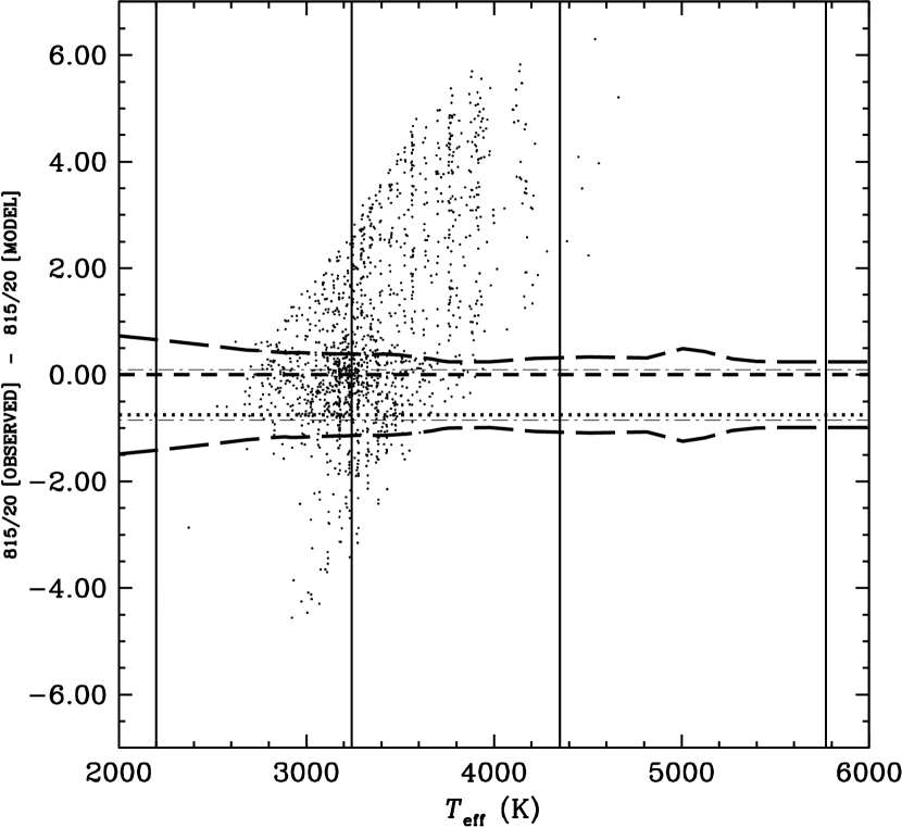
Figure 9: Difference between the observed 815/20 magnitude and that computed from the derived mass and $T_{\rm eff}$, as a function of $T_{\rm eff}$. The four vertical lines are at the positions of L0, M5, K5 and G5 dwarfs (left to right). The dotted line (at $-0.753$) represents the error due to the possible presence of unresolved binaries at, the dashed-dotted lines represents the error on the magnitude determination and the long dashed lines represents the uncertainties on the age and distance of IC 2391. (The short-dashed line just traces zero).

As indicated in §2.4, our determination of $T_{\rm eff}$ is based on the energy distribution of each object and is independent of distance. The membership status is determined by comparing the observed magnitude of a given object in a band with the magnitude predicted based on its derived $T_{\rm eff}$ and IC 2391’s isochrone. (The premise is that the predicted magnitude of a background contaminant would be lower - brigher - than its observed magnitude and higher for a foreground contaminant.) In order to avoid removing unresolved binaries that are real members of the cluster, we keep all objects with a computed magnitude of up to 0.753 mag brigher than the observed magnitude. In this procedure, we are also taking into acount photometric errors and uncertainties in the age and distance determinations of IC 2391. This is represented in Figure 9. Combined with the rejection of contaminants based on proper motion, this selection step reject 89.2% of the 33 794 candidates obtained from the CMD and colour-colour diagrams.

4 RESULTS OF THE SURVEY

The final selection gives us 954 photometric candidates for outward fields (namely fields 43, 46, 47, 48 and 49), 499 photometric candidates for the four deep fields (15, 20, 27 and 32, with filters $R_{\rm c}$, 770/19, 815/20, 856/14 and 914/27) and 1 734 for all other radial fields (observed with filters $R_{\rm c}$, 815/20, 914/27 and $J$). (We present in §5.3 a discussion of the contamination of the radial fields.) All our photometric candidates are presented in Table 2. Objects are given the notation IC 2391-WFI-ZZ-YYY where ZZ is the field number and YYY a serial identification number (ID). Only the first 10 rows of the tables are shown, the remainder available online. We also compare in Table 3 all objects in our sample which are also confirmed as cluster members from Barrado y Navascués et al. (2004) and Dodd (2004) and was detected by the X-ray Multi-Mirror Mission (XMM-Newton). We see a good agreement between $T_{\rm eff}$ from our photometric data and from Barrado y Navascués et al. (2004), where only the colour ($R-I$)_c was used to compute $T_{\rm eff}$.

Not all candidate members from previous studies, detected in our survey, are members of IC 2391 based on our photometric selection. As pointed above, a cluster member presented in this work is an object that satisfies all four steps of our selection procedure. For instance, among the two objects detected in our survey which are also cluster candidates by Patten & Pavlovsky (1999), one is recovered by our selection (object number 8). From 10 objects classified as candidate members from spectroscopy and photometry by Barrado y Navascués et al. (2004), 5 are recovered in our selection: objects CTIO-038 and -091 fail the colour-colour diagrams test and objects CTIO-041, -049 and -091 fail the predicted magnitude vs. observed magnitude test. One possible source of disagreement could be the use of H$\alpha$ by Barrado y Navascués et al. (2004) as a membership criteria (see §6.1 for further discussion of this issue).

A total of 53 objects classified as cluster members by Dodd (2004) based on proper motion and photometry were detected in our survey. However, one of Dodd objects is recovered in our survey (object number 155, also identified as CTIO-152). This is also the only matchs, within 4 arcsec, with the cluster members of Barrado y Navascués et al. (2004). Considering the size of the window used for their proper motion selection (in milliarcsec, -28$\geq$$\mu_{\alpha}$cos$\delta$$\geq$-20 and +20$\leq$$\mu_{\delta}$$\leq$+28) and the order of the error on the known proper motion of IC 2391 ($\lesssim$2 miliarcsec in $\mu_{\alpha}$cos$\delta$ and $\mu_{\delta}$, see §3.3 below), one could suspect some contamination by field stars. This can be confirmed by the large scatter in the CMDs of IC 2391 presented by Dodd (2004) below $R$$\sim$12 and $K$$\sim$10 in Figure 3 and 4 respectively. Another survey on IC 2391 based on proper motion was performed recently by Platais et al. (2007). However, as discussed in §3.1, no objects from this work were detected in our survey.

Only two objects listed Table 2 from Marino et al. (2005) (IC 2391 members observed with XMM-Newton) were also detected by our survey (source number 86 and CTIO-130), but neither objects is recovered by our photometric selection. The first one is a source that overlaps with VXR53 from Patten & Simon (1996) and was identified as a suspected cluster member, and also overlaps with CTIO-126 from Barrado y Navascués et al. (2001) and was classified as a cluster member (however, there was no spectroscopic follow-up of CTIO-126 by Barrado y Navascués et al. 2004). This object is not recovered in our selection because this candidate fail the observed magnitude vs. predicted magnitude test. Another object presented by Marino et al. (2005) (observed only by the MOS cameras onboard XMM-Newton, but not by the pn camera) is CTIO-130, but they noted that this star has $J$ and ($J$-$K$) values incompatible with the IC 2391 main sequence.

4.1 Effect of Background Contamination on Candidate Selection

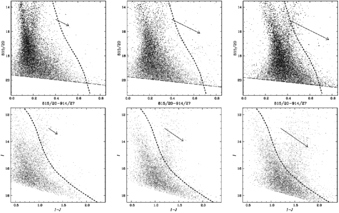
Figure 10: CMDs of 3 fields from our survey (top, from left to right, fields 40, 01 and 09) and 3 CMDs from the same fields using DENIS data (bottom, $I$ versus $I$-$J$). The NextGen isochrones is also shown. We clearly see a colour shift of the (field star) locus between these fields in our data, as well in the DENIS data. For all panels, the arrows represents the reddening vectors based on $E$($B$–$V$) towards each fields.

In comparing the CMDs for different fields, we discovered something peculiar (Figure 10, top 3 panels). We see a shift in the colours of the bulk of the (field) stars from field to field, something we also observe in other colours. The comparison of the amplitude of this shift (for a given magnitude interval) with observational parameters such as nights, airmass, seeing and 10$\sigma$ detection limit shows no correlation and there is no other indication of reduction problems. We did, however, find a correlation of the colour shift with the Galactic longitude b. However, in order to verify that these shifts where real, we obtained DENIS photometry (Deep Near Infrared Survey of the Southern Sky) in $I$ and $J$ band for the same fields presented in Figure 10, which are field 01, 09 and 40. We can see that the shift in the colours of the bulk of the (field) stars is also observed in the DENIS data (Figure 10, lower 3 panels).

Although reddening is negligible for objects in IC 2391, this is not the case for background objects, and these constitute most of the stars in our sample. Due to the high variation of the background extinction in this direction of the Galactic disk (Schlegel et al. 1998) – the cluster is centered at l=270.4 b=-6.9 – some variation in the CMD locus could be extinction-induced variations in the background stars. In Figure 11 (left), we plot the reddening $E$($B-V$) in our fields against the median of the colour 815/20-914/27 (in a bin of magnitude of 15 $<$ 815/20 $<$ 16) for all our fields. The colours vary by as much as 0.25 mag. To better illustrate the spatial variation of the background extinction, Figure 11 (right) shows the position of the fields of our survey overplotted with the $E$($B$-$V$) extinction map of Schlegel et al. (1998). This colour gradiant of the background stars has not been reported in previous surveys of IC 2391 (Dodd 2004; Barrado y Navascués et al. 2001; Patten & Pavlovsky 1999). It can be expected that Barrado y Navascués et al. (2001) and Patten & Pavlovsky (1999) didn’t observed such shift in colour since their survey cover a smaller area (2.5 and 0.8 sq. deg. respectively) of the sky compared to our 10.9 sq. deg. coverage.

4.2 Mass Function

The mass function, $\xi$(log₁₀M), is generaly defined as the number of stars per cubic parsec (pc³) in the logarithmic mass interval log₁₀M to log₁₀M + $d$log₁₀M. Here, we do not compute the volume of IC 2391 so instead we present a MF using the total number of objects in each 0.1 log₁₀M bin per 1 000 arcmin², starting at the mass bin log₁₀M=-1.65 ($\sim$0.02 M_⊙). The mass functions computed here are all system mass functions since we don’t make any corrections for binaries. We analyse the radial variation of the MF using the fields with photometry with the filters $R_{\rm c}$, 815/20, 914/27 and $J$ (Figure 12). Mass functions were computed over three regions: for fields between 0.5^∘ to 1.5^∘ of the cluster center (which corresponds to 1.3 pc and 3.8 pc respectively); for the annulus from 1.5^∘ to 2.1^∘ (which corresponds to 5.4 pc); for fields outside of 2.1^∘. We have also computed a MF for all fields within 2.1^∘ of the cluster center to help radial variation analysis and present this as our estimation of the MF for IC 2391. Furthermore, we have measured the MF for the five outward fields and also for the four deep fields (Figure 13).

Since the radial fields were also observed with $R_{\rm c}$ in addition to the filters used for both the radial and outward fields, we use this to estimate the (additional) contamination in outward fields relative to the radial fields for each mass bin. To do so, we performed a photometric selection for our radial fields using only the filters available in the outward fields (815/20, 915/27 and $J$). We compared the MF computed from this with the MF from the outward fields and obtained, for each mass bin, the number of object that would have been rejected if we would had an additional $R_{\rm c}$-band observation. (Here we make the assumption that the true MF should be the same in the radial and outwards fields.)

In Figure 13 (left panel) we present the uncorrected MF of the outward fields and the corrected MF of the outward fields (right panel). It is not possible to perform such corrections for the deep fields.

Useful (and simple) parametrizations of the mass function include the power law of Salpeter (1955) and a lognormal

$$\xi(\textrm{log}_{10}\,\textrm{M})=k\cdot\textrm{exp}{\biggl{[}-\frac{(\textrm{log}_{10}\,\textrm{M}-\textrm{log}_{10}\,\textrm{M}_{0})^{2}}{2\sigma^{2}}\biggr{]}},$$ (4)

where $k$=0.086, $m_{0}$=0.22 M_⊙ and $\sigma$=0.57 was derived for the Galactic field by Chabrier 2003). Fitting the lognormal mass function to our data for all fields within 2.1^∘ of the cluster center, we obtain $k$=10.7$\pm$3.2, $m_{0}$=0.13$\pm$0.03 M_⊙ and $\sigma$=0.46$\pm$0.07. This is overplotted in Figure 13.

If we assume that the lognormal fit of the MF describe the behaviour of the population in the mass range 0.02–0.9 M_⊙ in IC 2391, the total number of object expected is 3 985 for a total mass of 679 M_⊙. (In §5.3 we will discuss again the total number of object and total mass, following an estimation of the contamination for each mass bin in the MF of the radial fields.)

We present in Figure 14 the MF for all fields within 2.1^∘ of the cluster center and from other open clusters with similar ages (NGC 2547, $\sim$30 Myr; IC 4665, 28^+7.3_–6.6) Myr based on Li depletion boundary, Manzi et al. 2008). We also show on Figure 14 the MF of IC 2391 as determined in previous work (i.e. from Barrado y Navascués et al. 2004 and Dodd 2004). All were normalized to the Galactic field star MF at 0.3 M_⊙.

5 ANALYSIS AND DISCUSSION OF THE MASS FUNCTIONS

In the following subsection, we discuss the mass function derived from the deep fields and from outward fields only. The other fields are used to study the radial variation of the MF and are subject of further discussion in the following two subsections. We complete this section with a discussion of the contamination rate by non-cluster members.

5.1 Mass Function of the outward fields and of the deep fields

Considering the fact that only three bands were used for the outward fields, and thus fewer constraints imposed, we expect that the number of photometric candidates would be larger per unit area than the other fields. The MF (Figure 13, left panel) shows more low mass objects (compared to the MF of the radial field, for masses below $\sim$ 0.15 M_⊙), a similarity with the radial MF from 0.13 to 0.3 M_⊙, and again more stellar objects in the mass range 0.5 to 0.8 M_⊙. The corrected MF (Figure 13, right panel) shows a better agreement with the radial MF.

The MF from the deep fields (Figure 13) agrees with the mass function of the radial fields within 2.1^∘ from cluster center in the mass range 0.05 to 0.1 M_⊙ and above 0.2 M_⊙. However, there is more substellar objects below 0.05 M_⊙.

The rise of the MF for objects below 0.05 M_⊙ was also observed in IC 2391 by Barrado y Navascués et al. (2004). In their work, the MF was computed with objects that were selected as cluster members based on $R_{\rm c}$, $I_{\rm c}$, $J$, $H$ and $K$ photometry. Since their NIR photometry was taken from 2MASS, no data are available for objects fainter than $I_{\rm c}$$\lesssim$19 (10$\sigma$ detection limit of 2MASS is at $J$$\sim$15.8). As a result, their selection for fainter objects was based on $R_{\rm c}$ and $I_{\rm c}$ photometry only. In our case, although $J$ band photometry is available for the outward fields, no $R_{\rm c}$ photometry is available. Thus Barrado y Navascués et al. (2004) used a relatively short baseline ($R_{\rm c}$–$I_{\rm c}$) for their selection, as did we in our outward fields (815/20, 914/27 and $J$), both of which are considerably shorter than the baseline we used in the radial fields ($R_{\rm c}$, 815/20, 914/27 and $J$). This situation is also observed in the MF of the deep fields (where $R_{\rm c}$ band photometry is available, but no $J$ band photometry). Only the fields observed with $R_{\rm c}$ and $J$ as well (i.e. a longer baseline) show no significant rise of the MF below 0.05 M_⊙ (Figure 13, left panel). Since no red giants were observed in our spectroscopic follow-up of the two deep fields 15 and 20 (§6), we conclude that this increase is an artefact due to contamination by M–dwarfs. In this low mass regime (for objects with mass $\lesssim$0.05 M_⊙), a long spectral baseline (including, for instance, $R_{\rm c}$ and $J$) is needed to efficiently remove contaminations, as it allows a better determination of the energy distribution. This is confirmed when we compare the corrected and uncorrected MFs of the outward fields (Figure 13).

The rise in the MF over 0.5–1.0 M_⊙ is observed in the outward fields but not in the deep fields (Figure 13). Jeffries et al. (2004) present the MF of the open cluster NGC 2547 and also noticed a rise in the 0.7–1.0 M_⊙ interval (Figure 14). This rise, also observed in the luminosity function as a large peak at 12 $\lesssim$ $I_{\rm c}$ $\lesssim$ 14.5, they attribute to contaminating background giants. This would be consistent in the fact that we see this in the radial fields (see Figure 12) but not in the deep fields (Figure 13). Indeed, as we discuss later in §6, no red giants were found in our spectroscopic follow-up, confirming that the use of medium bands such as 770/19, 815/20, 856/14 and 914/27, and theoretical colours (Hauschildt et al. 1999b) are effective in removing background red giants. However, from the MF of the radial fields (including the outwards fields), the medium filters 815/20 and 914/27 alone, combined with wide band $R_{\rm c}$ and/or $J$, are less efficient at removing background giants. Therefore, the rise in the MF of the outward fields over 0.5–1.0 M_⊙ is related to the filters used, but is not a baseline issue.

We also observe on Figure 13 that two mass bins at $\sim$0.11 and $\sim$0.18 M_⊙ are significantly high compared to the other mass bins in the mass range 0.05–0.3 M_⊙. Considering that this is not observed in the MF of the radial field and in the corrected/uncorrected MF of the outward fields, we suspect that this is due to the selection procedure related to the deep fields so no conclusion should be made based on these two mass bins.

5.2 Radial Variation of the Mass Function at the Stellar and at the Substellar Regimes

From a first glance at Figure 12, we see that the two mass functions within 2.1^∘ (the points in the two left-hand panels) are somewhat similar. While there is some differences, these are not very significant compared to the difference between their common MF within 2.1^∘ (plotted as the histogram) and the MF in the outskirts of IC 2391 (beyond 2.1^∘) as shown in the right-hand panel. Indeed, the MF for $\theta$$>$2.1^∘ shows a significant deficiency of stellar objects from 0.1 to 0.3 M_⊙ (log₁₀M=-0.6) compared to the MF from the inner part of the cluster, whereas outside of this mass range there is no significant change with radius. Although we observe a number of objects in the highest mass bins at 0.5–0.7 M_⊙ (log₁₀M=-0.3 to -0.15), we concluded (in §5.1) that this range of masses is subject to significant contamination by red giants, so no conclusion should be drawn from the radial variation of the MF in this mass interval.

In Figure 15 we present the cumulative mass function for the same three regions of the cluster presented in Figure 12. We again see the relative absence of objects from 0.1 to 0.3 M_⊙ (log₁₀M=-0.6) for the inner radii. A Kolmogorov-Smirnov test performed on these distributions indicates that there is only a 1.1$\cdot$10^-5 % probability of getting such a difference under the null hypothesis that the population at $\theta$$>$2.1^∘ is the same as that at $\theta$$<$2.1^∘, thus reinforcing the suggestion that the mass functions are significantly different.

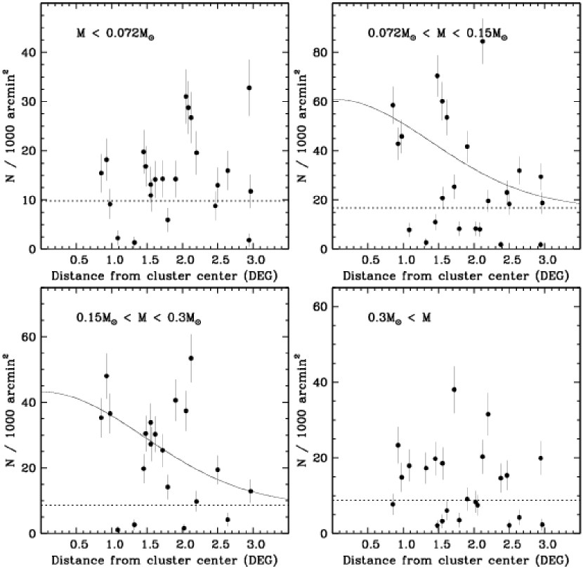
Figure 16: Radial profile of IC 2391 for four different mass bins as indicated in each panel. A King profile fit (King 1962) was used for the radial profile for 0.072 M_⊙ $<$, M $<$ 0.15 M_⊙ and 0.15 M_⊙ $<$, M $<$ 0.3 M_⊙ (solid line). An estimation of the background contamination for each mass bin is given by the horizontal dotted line. In the panel of 0.15 M_⊙ $<$, M $<$ 0.3 M_⊙, the four data points at N = 0 indicate that no object was detected in that mass range for these fields (fields 03, 04, 31, 40 and 41, where 03 and 41 are at a similar distance of $\sim$2.94^∘ from cluster center).

To help the analysis of the radial variation as a function of mass, we also present on Figure 16 the radial profile of IC 2391 using the radial fields for four different mass bins: M $<$ 0.072 M_⊙, 0.072 M_⊙ $<$ M $<$ 0.15 M_⊙, 0.15 M_⊙ $<$ M $<$ 0.3 M_⊙ and 0.3 M_⊙ $<$ M. (It is not surprising that a fit for the most massive stars is not possible since the core radius is at 0.35^∘ and we do not have any radial fields closer than 0.8^∘.) For the second and third radial profile, we fit a King profile (King 1962), where the fit give us a maximal number density at the center of 27.7${}^{+29.9}_{-17.8}$ and 26.1${}^{+16.9}_{-11.3}$ members per 1 000 arcmin² and a full width at half maximum of 1.39^∘${}^{+0.44}_{-0.23}$ (or 3.5 pc${}^{+1.2}_{-0.5}$) and 1.45^∘${}^{+0.47}_{-0.24}$ (or 3.7 pc${}^{+1.2}_{-0.6}$), respectively. This is purely for illustration purposes, as it is clear that this is not a good model for this mass profile.

In Figure 12 we do not see any significant radial variation of the MF in the substellar regime. The radial profile of the substellar population in Figure 16 also indicates no significant radial variation. On the other hand, we do see reasonable evidence for a radial variation for masses above 0.072 M_⊙. From this radial profile and the mass functions already discussed, we can conclude that the spatial distribution of the BD population is uniform compared to the stellar population (from 0.072 to 0.3 M_⊙), which is more clustered within $\theta$$\sim$2^∘.

Kumar & Schmeja (2007) also found the stellar population to be more clustered than the substellar population in the clusters IC 348 and Trapezium. This would favour the ejection scenario for forming BDs if the BDs have a higher velocity dispersion than the stars (Kroupa & Bouvier 2003), because the higher velocity from ejection creates a more uniform spatial distribution for the BDs compared to the stars. However, the two clusters of Kumar & Schmeja (2007) are both younger than 3 Myr, while IC 2391 has an age of 50 Myr, some $\sim$3 times older than its crossing time ($t_{cross}=$17 Myr). We can expect that if BDs have a higher velocity dispersion than stars, then in an older cluster most of the BDs with velocity dispersion greater than the escape velocity could have escaped the cluster already (Moraux & Clarke 2005).

The homogeneous distribution of the substellar objects compared to the more clustered stellar population could be instead a signature of mass segregation through dynamical evolution or of primordial origin. We have indicated previously that mass segregation via dynamical evolution could occur on a timescale of order one relaxation time (Bonnell & Davies 1998), or even less (Allison et al. 2009). Considering that the cluster is only three times older than its crossing time, which may be insufficient for significant dynamical evolution, it is difficult to make an inference on the BD formation mechanism from the radial MF variation given the uncertainty about to what extend the cluster has evolved dynamically. If it could be demonstrated that the cluster is dynamically unevolved and that the BDs have a higher velocity dispersion than the stars, then our observations are consistent with BD formation by the ejection hypothesis.

5.3 Contamination by non-members

Possible point source contaminants other than field M–dwarfs include red giants and high redshift quasars (Caballero et al. 2008). However, as pointed out in §5.1 and in our spectroscopic follow-up (see below in §6.3), the use of medium band filters and theoretical colours is efficient at removing potential background red giant contaminants. As for the high redshift quasars (for instance at $z$ $\sim$ 6), their spectral energy distribution is similar to mid-T dwarfs and moreover, they are rare (Caballero et al. 2008). Considering that our faintest targets are early L–dwarfs, the MF should not be affected by contamination by quasars.

Here we present an estimation of the contamination in our photometric survey based on the radial fields. First, we used the radial profile of IC 2391 using the radial fields for four different mass bin (Figure 16). We assumed that near the tidal radius ($\sim$2.89^∘), the number of objects per 1 000 arcmin² should be zero. From this, we computed that we can expect a contamination of $\sim$8.8 objects per 1 000 arcmin² for masses above 0.3 M_⊙, $\sim$8.8 objects per 1 000 arcmin² in the mass range of 0.15 M_⊙ $<$ M $<$ 0.3 M_⊙, $\sim$16.7 objects per 1 000 arcmin² in the mass range of 0.072 M_⊙ $<$ M $<$ 0.15 M_⊙ and $\sim$9.8 objects per 1 000 arcmin² in the substellar regime. If we use the same assumptions about the lognormal fit of the MF, the new total number of object expected in IC 2391 is 1 954 for a total mass of 308 M_⊙.

6 PRELIMINARY SPECTROSCOPIC FOLLOW-UP

Here we present the results of a preliminary spectroscopic follow-up of some photometric candidates. As explained in the previous section, the main sources of contamination in our photometric selection are background red giants and field M–dwarfs. We have also shown in §4.1 that, because of extinction, background contamination is non-uniform. We therefore need to refute or confirm membership status with optical spectra. For this task we used the fiber spectrograph HYDRA. It is not possible to cross fibres with this instrument, so we have not yet been able to observe all candidates in a given field. (It is our intention to eventually obtain spectra of all candidates.) The data reduction was described in §2.5 while the spectral type and luminosity class determination was presented in §2.6. The spectroscopic $T_{\rm eff}$ was obtained using the spectral type and the temperature scales of Luhman (1999) while each mass was derived from $T_{\rm eff}$ using our isochrone for IC 2391. We discuss membership determination based on optical spectra below in §6.2.

Among the spectra obtained, 17 had a signal-to-noise ratio (SNR) higher than 5. These are presented in Figure 17. Table 4 provides the derived parameters (spectral type, $T_{\rm eff}$ and mass) and the SNR. Objects are given the same notation as the photometric candidates : IC 2391-WFI-ZZ-YYY where ZZ is the field number and YYY a serial identification number (ID). Table 5 gives details of an object confirmed as cluster members by Barrado y Navascués et al. (2004), including their SpT and $T_{\rm eff}$ determination, for which we also have a spectra.

6.1 Contaminating H$\alpha$ nebula emission

We mentioned in §2.5 the presence of contamination at H$\alpha$ in sky spectra. As these spectra are used for background subtraction (we have fiber spectra), there are potential difficulties in measuring the stellar H$\alpha$ line. We now discuss this issue.

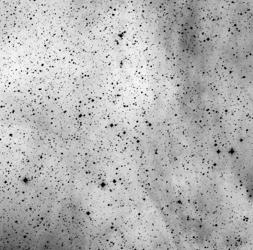
Figure 18: Left. H$\alpha$ emission (median counts) in fields of size 200 x 200 arcsec from the SuperComsos Survey at the location of our sky fibers, plotted against the flux (in counts) of the H$\alpha$ emission line we measured in our sky fibers in the HYDRA pointing of field 20. Right. H$\alpha$ observations from SuperCOSMOS towards field 20 (images of 35$\times$35 arcmin).

In producing a high-resolution atlas of night-sky emission lines with the Keck echelle spectrograph, Osterbrock et al. (1996) observed an H$\alpha$ emission line at high Galactic latitudes which they concluded was due to diffuse interstellar gas emission (the closest atmospheric emission observed were two OH lines at 6553.617 Å  and 6568.779 Å ). From the AAO/UKST SuperCOSMOS H$\alpha$ Survey (SHS, Parker et al. 2005), we have also noticed high variations of H$\alpha$ emission at low Galactic latitude. We used the SHS to estimate the H$\alpha$ emission at each position of our sky fibers (by taking a median of the flux over a 200 x 200 arcsec window). The frames are flat-field corrected but not flux calibrated, so we retain the unit of (photon) counts. In Figure 18 we plot this against the flux (in counts) of the H$\alpha$ emission line of our background spectra for field 20. While there is no strong evidence for a correlation, we nonetheless see a significant variation of the H$\alpha$ emission. As this clearly prevents a reliable background subtraction of the H$\alpha$ line, we choose not to draw any conclusions on membership status based on this line. We must therefore question its use by Barrado y Navascués et al. (2004) for this purpose (who used the same instrument for the same cluster). For further observations of objects in direction of IC 2391 using fiber-fed spectrograph, we recommend background subtraction to be performed in a similar way as the one done by Carpenter et al. (1997), where the same fibers for the science targets were also used for sky subtraction but shifted 6 arcsec away.

6.2 Membership Determination

We use the Li I line at 6708 Å to help confirm substellar status of photometric candidates and to establish membership of IC 2391. Lithium can be observed in young, more massive stars with radiative interiors because of less efficient mixing than in fully convective low mass stars (e.g. Manzi et al. 2008). Lithium may still even be present in the atmospheres of young, fully convective low mass stars, if they are young enough that not yet all the lithium has been ”burned” (Manzi et al. 2008). Older, lower mass BDs ($\lesssim$0.065 M_⊙) never achieve core tempertures high enough to burn lithium and so preserve their initial lithium content (Rebolo et al. 1996). Here we assume that field stars (with M$\gtrsim$0.072 M_⊙) are too old to still retain lithium in their atmospheres. Hence we take the presence of the LiI line in candidates with M$\lesssim$0.072 M_⊙ as an indicator of membership in IC 2391, as only cluster members fainter than the Lithium depletion boundary ($I_{\rm c}=$16.2 mag, Barrado y Navascués et al. 2001) are young enough to retain Lithium.

The sodium doublet at 8200 Å is a gravity indicator, so is sometimes used to exclude field stars. Specifically, its equivalent width (EW) is sensitive to log $g$ (Martín et al. 1996) and because BDs contract as they age, log $g$ will increase. Because field late M–dwarfs (which have similar colours to M dwarf cluster members) will generally be much older and so more evolved, they will have larger EWs in this line (for a given chemical composition). We use the EW measurement of CTIO-046 from the Barrado y Navascués et al. (2004) survey as a lower limit on EW values for M-dwarfs to be non-members. (This object was defined as a non-member based on various criteria and had $W$(NaI)=7.3$\pm$0.2 Å). It can be argued that, since surface gravity changes with mass, the limit EW(NaI)=7.3Å could also change with mass. Based on our isochrone of IC 2391, from 0.04 to 0.2 M_⊙ (which is the mass range of our spectroscopic follow-up), the surface gravity will varies only from log g = 4.65 to 4.72 ($\delta$ log g = 0.07).

The spectral resolution is sufficient to provide an estimate of the radial velocity. As for the radial velocity criteria, we exclude candidates which differ significantly ($\pm$3$\sigma$) from a recent determination of the cluster’s radial velocity (16$\pm$3 km/s, Kharchenko et al. 2005, where $\sigma$ is the the error of the radial veolicty of IC 2391 added in quadrature with the error of our candidates). We didn’t used radial velocity measurment for which errors exceed 30 km/s, which is ten time the error on the radial velocity of IC 2391.

Finally, we use the SpT determination to obtain $T_{\rm eff}$ and masses for each spectrum. In order to be confirmed as a (spectroscopic) cluster member, the spectroscopic $T_{\rm eff}$ and must agree with the photometric $T_{\rm eff}$ to within 200 K.

In Table 6 we again present all objects from Table 4, but with physical parameters and with membership status based on photometry and spectroscopy (i.e. which satisfy our spectroscopic criterium). We don’t reject objects below which does not present a feature of LiI due to low SNR if the other criteria are satisfied (e.g. IC2391-WFI-15-005).

6.3 Discussion of the spectral data

Of the 17 photometric candidates observed with a SNR higher than 5, 9 are spectroscopic members of the cluster. We find no red giants in our spectral sample, which demonstrates that our choice of filters and selection procedure is efficent at minimizing this contamination. Since our spectroscopic follow-up covers only part of the mass range used for the mass function calculation in §5, it is not possible to compute a new MF with corrections applied at each mass bin. It is expected that the contamination rate would be different for other mass range and fields (for different filter combinations). One of our spectral targets was observed by Barrado y Navascués et al. (2004): CTIO-62, which has the label IC2391-WFI-20-067 in our survey. We agree with Barrado y Navascués et al. (2004) on the status (cluster member) of this object.

Another of our spectral targets, IC2391-WFI-20-001, shows Lithium even though this object has an inferred mass above the stellar/substellar boudary (spectroscopic mass of 0.079 M_⊙ and a photometric mass of 0.089 M_⊙). The lithium depletion boundary has been estimated to be at $I_{\rm c}=$16.2 mag (Barrado y Navascués et al. 2001), which corresponds to an effective temperature of about 3 000 K based on our isochrones of IC 2391. As the cluster is not that old, the lithium depletion boundary lies well above the substellar boundary, so its not surprising to see a trace of Lithium in the spectrum of this object (which has a magnitude of $I_{\rm c}=$16.681 mag).

Although we obtained for IC2391-WFI-20-024 the same spectral type as for IC2391-WFI-20-029, we consider this object as a member of IC 2391, but to have a mass slightly above the substellar. Its photometry gives $T_{\rm eff}$ = 2958 K and M = 0.081 M_⊙, with a predicted magnitude of 815/20 = 16.445 mag. If this object were an unresolved binary, we would expect its observed magnitude to be brighter than its predicted one, which is not the case (observed magnitude of 815/20 = 16.520 mag). Also, it should be noted that this object was observed with a fibre with poor spectral response below 6800 Å  (which is why we don’t show it in Figure 17). Although this does not affect the PC3 index used for the SpT determination (which covers 7540 Å  to 7580 Å, and 8230 Å  to 8270 Å), it does influence the reduction process (including the throughput correction, illumination correction, extraction of the spectra and flux calibration). Therefore, we consider its SpT uncertainty to be larger (two subtypes rather than one).

6.4 Discovery of new brown dwarf members of IC 2391

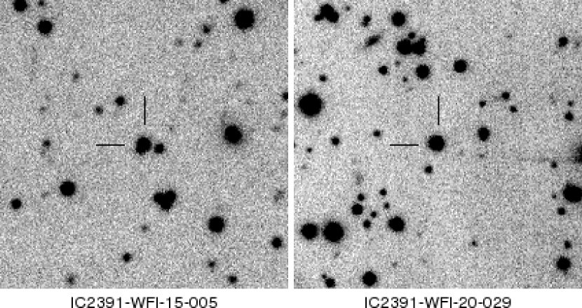
Figure 20: Finding charts of the two new brown dwarf members of IC 2391 (from 815/20 images). The panels are 3.5$\times$3.5 arcmin with North up and East to the left.

Of the 17 spectral targets, we assign as brown dwarfs two in IC 2391, on the basis of spectroscopic confirmation, and having both photometric and spectroscopic masses below 0.072M _⊙. These are new discoveries. These objects are IC2391-WFI-15-005 and IC2391-WFI-20-029. Table 7 lists their parameters, Figure 19 shows their spectra and Figure 20 contains the finding charts. We can see in Figure 19 that H$\alpha$ is not visible in IC2391-WFI-20-029, so it would be designated as non-members by Barrado y Navascués et al. (2004). Considering that the MF from our radial fields is similar to that of the deep fields in the mass range of these two new objects (from 0.045 to 0.07 M_⊙), then if we used the same selection method, then statistically we would expect to find two brown dwarfs in the same mass range in the other two deep fields, and about 31 in all of the radial fields.

7 CONCLUSIONS

We have performed a multi-band photometric survey over 10.9 square degrees of the open cluster IC 2391, and completed a preliminary spectroscopic follow-up of brown dwarfs and very low mass stars candidates from two of the WFI fields. Our objective was to study the mass function of this cluster, and in particular its radial dependence. We observed a radial variation in the MF from 0.072 to 0.3 M_⊙, but we do not observe a significant radial variation in the mass function in the substellar regime. This comparative lack of radial variation of the substellar mass function is in favour of the ejection scenario for forming brown dwarfs, but considering that IC 2391 is $\sim$3 times older than its crossing time, we might expect that most of the brown dwarfs with velocity dispersion greater than the escape velocity could have already escape the cluster. On the other hand, the rather homogeneous distribution of the substellar objects and the clustered distribution of stellar objects within $\theta$$\sim$2^∘ could be a signature that mass segregation via dynamical evolution has occurred in IC 2391, or that this mass segregation is of primordial nature. We have concluded that if this cluster is dynamically unevolved and if the brown dwarfs have a higher velocity dispersion than the stars, then our observations are consistent with brown dwarf formation by the ejection hypothesis.

In addition to the radial study, we derived a mass function from four central deeper fields as well as from five fields near the edge of the cluster observed with only three filters (the outward fields). In both cases we see an apparent rise in the number of objects below 0.05 M_⊙ (log₁₀M=-1.3), but we concluded that this is an artefact of residual contamination by field M dwarfs. This was also seen by Barrado y Navascués et al. (2004). The fact that we don’t see this rise in the radial fields is because they were observed with both the $J$ and $R_{\rm c}$ filters in addition to the medium band filters. This longer spectral baseline permits a better determination of the energy distributions and thus helps the rejection of objects (in particular field M dwarfs) based on observed magnitude vs. predicted magnitude from models.

Another apparent rise in the MF over the 0.5–1.0 M_⊙ interval (also observed by Jeffries et al. 2004 for NGC 2547) is due to background giants. Red giant contamination may be reduced by using medium bands such as 770/19, 815/20, 856/14 and 914/27, and theoretical colours of red giants (Hauschildt et al. 1999b). Our spectroscopic follow-up has confirmed that selection based on these filters resulted in no red giant contaminants among our sample of spectra.

We see some variation in the colours of the main (field star) locus which we attribute to variable extinction affecting the background stars. This underlines the need for spectroscopic observations in this cluster in order to confirm membership and/or brown dwarf status in individual cases.

We have performed a preliminary spectroscopic follow-up of photometric cadidates in two of our deep fields (0.5 sq. degrees). Of 17 photometric candidates, we confirm 9 objects (i.e. half) as true cluster members. Of these, two are new brown dwarf members of IC 2391 (in the sense that they fufill our spectroscopic and photometric criteria). Using our derived mass functions for the deep and radial fields, we expect there to be two more brown dwarfs in the mass range 0.045 to 0.07 M_⊙ in the other deep fields and up to 31 in all the other radial fields in the same mass range.

Finally, we find that the H$\alpha$ line cannot be used as a membership criterion from fiber spectroscopy at low spectral resolution (spectral dispersion of 1.14 Åper pixel) because of spatially variable diffuse H$\alpha$ emission. This prevents reliable sky subtraction around this line when using a fiber spectrograph with fibers assigned for sky subtraction.

Figure 1: Area covered by our survey of IC 2391. The four thick squares are the deep fields, the dotted squares are the outward fields and the others are the radial fields. The circles have radii of 1^∘, 2^∘ and 3^∘ from the cluster center.

Figure 2: Transmission curve of the filters used in our survey compared to the synthetic spectrum of a brown dwarf with $T_{\rm eff}$ = 2300 K, log g = 4.5 and solar metallicity (NextGen model).

Figure 3: Estimation of the completeness limit for the radial part of our survey using the $J$ band (left) and of the deep part using 914/27 (right). The tick lines give best linear fit before the turn off; the vertical tick dotted line is the 10 $\sigma$ detection limit and the vertical thin line is the magnitude for which saturation start to occur in the short exposures.

Figure 4: Spectrum used for sky subtraction of our spectroscopic data. Note the H$\alpha$ (nebula) emission line with equivalent width of $W$(H$\alpha$) = 48 Å.

Figure 6: Two colour-colour diagrams of objects that are candidates based on our first selection (from field 01). Isochrones and objects from Barrado y Navascués et al. (2004) (triangles), Dodd (2004) (squares) and XMM-Newton (circle) are as shown in Figure 5. The thin lines represent the colour of possible background red giant contaminants. The colour-colour diagram on the left is therefore not suited for further candidate selection since the isochrone is spanned by the colour grid of the red giants (which is not the case for the colour-colour diagram on the right). In each panel, the thin solid lines next to the isochrone represent the selection curve.

Figure 7: Colour sensitivity to effective temperature for the medium band filter 914/27. The vertical lines represents are at the approximate effective temperatures for spectral classes M5V (dash-dotted line) and K5V (long-dash line). We can see that there is no variation at all for 815/20-914/27 compared to other colours at the L0V and M5V regime.

Figure 8: Left. Proper-motion diagram from our survey (in milliarcsec per year). IC 2391 is at (-25.0,+23.0), which is taken from the literature (§3.3). The typicaly error bar of individual objects in our survey is shown. For clarity, only one object out of five is shown. Right. Contour plot of the same data.

Figure 11: Left. $E(B-V)$ towards all our fields (from the Schlegel et al. 1998 extinction map) plotted against the median 815/20-914/27 stellar colour in those fields. Right. Position of the fields of our survey overplotted by the $E$($B$–$V$) extinction map of Schlegel et al. (1998). The contour separation is 0.2 mag.

Figure 12: MF based on photometry for all radial fields. The 10$\sigma$ detection limit is shown as a vertical dashed line. Dots in each panel represent the MF of (left) fields within 1.5^∘ of the cluster center, (center) fields within the annulus from 1.5^∘ to 2.1^∘ and (right) the MF of fields outside of 2.1^∘. Error bars are Poissonian arising from the number of objects observed in each bin. The histogram is the MF for all fields within 2.1^∘ of the cluster center. The vertical thin dotted line is the mass for which saturation start to occur in the short exposures. (The total area covered for each panel, from left to right, is 6 637, 9 539 and 5 609 arcmin².) Just for reference, the ordinate value of 1.13 for the the bin at log₁₀M=-0.85 (0.14 M_⊙) – the histogram peak – corresponds to 109 objects.

Figure 13: Left. Filled dots represent the MF based on the four deep fields (observed with the wide bands $R_{\rm c}$ and the medium band 770/19, 815/20, 856/14 and 914/27) and open dots represent the MF based on the outward fields (observed with the wide band $J$ and the medium bands 815/20 and 914/27). Also, we present the 10$\sigma$ detection limit, the MF of all fields observed in $R_{\rm c}$, 815/20, 914/27 and $J$ within 2.1^∘ from the cluster center and its log normal fit. The vertical thin dotted and thin dashed line lines are the mass for which saturation start to occur in the short exposures for outward and deep field respectively. Right. Same as the left panel, but the outward fields MF presented is the corrected MF.

Figure 14: MF of IC 2391 from our present work (empty dots, from all fields within 2.1^∘ from the cluster center), for IC 4665 (filled triangles) from de Wit et al. (2006) and for NGC 2547 (filled dots) from Jeffries et al. (2004). We also show the galactic field stars MF from Chabrier (2003) as a dashed line. We also present the MF of IC 2391 from Barrado y Navascués et al. (2004) (empty triangles) and from from Dodd (2004) (empty squares).

Figure 15: Cumulative number of cluster members within 1.5^∘ (dash-dotted line), within the annulus from 1.5^∘ to 2.1^∘ (dotted line) and outside of 2.1^∘ (tick line). The 10$\sigma$ detection limit is shown as an horizontal dash line. The vertical thin dotted line is the mass for which saturation start to occur.

Figure 17: Spectra used in our analysis.

Figure 19: Spectra of the eight newly discovered brown dwarf members of the IC 2391 cluster found in our survey. We also present, for each spectra, a new close-up on the Li and the NaI doublet.

Table 1: Description of observations.

Field	RA	DEC	Distance (∘)	Region name	$R_{\rm c}$	770/19	815/20	856/14	914/27	$J$
01	8:24:38.8	-51:18:16.5	2.966	radial	1500/23.5	-	1800/20.8	-	600/19.7	1820/17.8
03	8:28:10.8	-50:46:50.0	2.945	radial	1500/23.8	-	1800/20.5	-	600/19.7	1820/17.7
04	8:27:56.8	-52:07:47.9	2.084	radial	1500/23.9	-	1800/20.5	-	600/19.5	1820/17.5
05	8:29:06.5	-52:26:14.6	1.793	radial	1500/23.7	-	1800/21.1	-	600/19.8	1820/17.5
06	8:30:30.6	-51:38:59.1	2.051	radial	1500/23.8	-	1800/21.1	-	600/19.7	1820/18.0
08	8:32:01.8	-52:15:26.1	1.481	radial	1500/23.9	-	1800/21.1	-	600/19.9	1820/17.9
09	8:33:15.7	-50:39:24.6	2.640	radial	1500/23.9	-	1800/20.8	-	600/19.8	1820/18.0
10	8:33:20.3	-51:50:14.6	1.616	radial	1500/24.0	-	1800/21.0	-	600/20.0	1820/18.0
11	8:34:06.5	-51:24:35.9	1.904	radial	1500/23.5	-	1800/20.7	-	600/19.8	1820/17.9
12	8:34:02.3	-52:45:43.2	0.978	radial	1500/23.7	-	1800/21.1	-	600/20.0	1820/17.9
14	8:36:17.4	-50:38:44.9	2.498	radial	1500/23.4	-	1800/20.8	-	600/19.7	1820/17.9
15	8:38:31.6	-53:35:29.4	0.757	deep	3900/22.7	3900/20.9	3000/20.7	1500/19.7	3000/20.3	-
17	8:37:37.6	-51:34:05.6	1.552	radial	1500/23.6	-	1800/20.9	-	600/19.7	1820/17.5
18	8:38:11.5	-52:01:44.1	1.085	radial	1500/22.7	-	1800/20.9	-	600/19.5	1820/17.6
19	8:38:17.7	-50:58:08.4	2.121	radial	1500/24.0	-	1800/20.6	-	600/19.6	1820/17.7
20	8:38:45.1	-52:35:58.0	0.519	deep	3900/22.4	3900/20.8	8400/21.3	15678/21.1	3000/20.3	-
21	8:41:22.5	-52:14:04.7	0.854	radial	1500/23.8	-	1800/21.2	-	600/19.9	1820/17.7
22	8:40:50.6	-51:31:11.6	1.553	radial	1500/23.7	-	1800/21.1	-	600/20.0	1820/17.8
24	8:39:59.7	-54:14:24.0	1.170	radial	1500/23.8	-	1800/20.5	-	600/19.7	1820/17.9
26	8:40:16.2	-55:16:12.0	2.200	radial	1500/23.7	-	1800/20.6	-	600/19.7	1820/17.7
27	8:41:01.5	-53:50:51.7	0.789	deep	3900/22.5	3900/20.7	9300/21.5	7800/20.4	4800/20.7	-
28	8:41:46.0	-54:46:27.8	1.720	radial	1500/23.8	-	1800/21.1	-	600/19.8	1820/17.5
31	8:44:09.0	-55:27:58.0	2.464	radial	1500/23.6	-	1800/20.5	-	600/19.5	1820/17.5
32	8:44:10.1	-52:39:49.0	0.721	deep	3900/22.3	3900/20.9	8450/21.4	10500/20.7	4800/20.5	-
35	8:44:39.7	-54:21:53.7	1.453	radial	1500/23.5	-	1800/21.0	-	600/19.9	1820/17.2
37	8:45:54.4	-53:25:53.5	0.927	radial	1500/23.5	-	1800/21.1	-	600/19.7	1820/17.5
38	8:47:00.8	-53:55:12.1	1.323	radial	1500/22.5	-	1800/20.9	-	600/19.6	1820/17.7
40	8:48:02.4	-55:09:16.4	2.380	radial	1500/22.8	-	1800/20.6	-	600/19.6	1820/17.7
41	8:48:09.8	-55:46:27.3	2.942	radial	1500/22.7	-	1800/20.4	-	600/19.4	1820/17.7
42	8:49:10.6	-54:35:58.2	2.023	radial	1500/22.7	-	1800/21.1	-	600/19.9	1820/17.5
43	8:50:15.8	-53:23:37.1	1.540	outward	-	-	1800/20.5	-	600/19.3	1820/17.5
46	8:53:03.1	-54:23:52.2	2.318	outward	-	-	1800/20.5	-	600/19.6	1820/17.3
47	8:53:26.1	-53:52:29.4	2.127	outward	-	-	1800/20.9	-	300/19.3	1820/17.3
48	8:54:39.8	-53:29:44.4	2.203	outward	-	-	1800/20.5	-	600/19.7	1820/18.2
49	8:56:47.5	-54:17:22.5	2.742	outward	-	-	1800/20.7	-	600/19.6	1820/17.8

Note. — System notation is exposure time in seconds / 10$\sigma$ detection limit while – indicate that no observations was performed for that field in that filter. Distance give the distance of the field from cluster center (in degree). The 10$\sigma$ detection limit in $R_{\rm c}$ is smaller than for the deep fields, although the exposure time was higher. $R_{\rm c}$ observations of the deep field were done in January 2000, while the observations of the radial fields were done in April 2007. Condensation problems and non-photometric nights was reported for the January 2000 observation run.

Table 2: All photometric candidates of our survey

Field	ID	RA	DEC	$R_{\rm c}$	770/19	815/20	856/14	914/27	$J$	M	$T_{\rm eff}$	[815/20]
01	001	8:26:16.055	-51:02:52.32	19.645	$-$	16.706	$-$	16.292	15.023	0.057	2768	17.220
01	002	8:26:14.211	-51:02:47.64	18.426	$-$	16.200	$-$	15.920	15.145	0.104	3072	15.943
01	003	8:25:28.826	-51:13:56.71	18.866	$-$	16.383	$-$	15.998	14.909	0.081	2957	16.450
01	004	8:25:47.698	-51:06:25.26	18.848	$-$	16.332	$-$	15.953	14.969	0.078	2935	16.537
01	005	8:25:26.432	-51:03:59.27	18.359	$-$	16.077	$-$	15.771	14.962	0.096	3043	16.080
01	006	8:25:01.148	-51:03:37.82	19.574	$-$	16.953	$-$	16.582	15.446	0.072	2890	16.710
01	007	8:24:10.028	-51:07:26.14	19.283	$-$	16.735	$-$	16.341	15.427	0.076	2925	16.576
01	008	8:24:33.508	-51:05:35.22	18.764	$-$	16.437	$-$	16.094	15.130	0.093	3029	16.146
01	009	8:23:19.415	-51:32:35.82	19.900	$-$	17.106	$-$	16.655	15.618	0.065	2838	16.930
01	010	8:23:29.455	-51:32:00.48	18.373	$-$	16.076	$-$	15.762	15.014	0.094	3032	16.134

Note. — Table 2 is published in its entirety in the electronic edition of the Astrophysical Journal. A portion is shown here for guidance regarding its form and content. The error on the determination of masses and effective temperature are the following : $\Delta$$T_{\rm eff}$ = 140 K and $\Delta$M = 0.1 M_⊙ for stars (M $>$ 0.2 M_⊙), $\Delta$$T_{\rm eff}$ = 230 K and $\Delta$M = 0.05 M_⊙ for VLMS (0.072 _⊙ $<$ M $<$ 0.2 M_⊙), $\Delta$$T_{\rm eff}$ = 420 K and $\Delta$M = 0.02 M_⊙ for BDs (M $<$ 0.072 M_⊙). The magnitude [815/20] is the predicted magnitude based on photometric determination of $T_{\rm eff}$ and mass.

Table 3: Objects from Barrado y Navascués et al. (2004), Dodd (2004) and detected by XMM-Newton which are photometric candidates in our sample

Field	ID	RA	DEC	815/20	M	$T_{\rm eff}$	[815/20]	NAME	$Ic$	($R-I$)$c$	$T_{\rm eff}$
18	006	8:38:47.074	-52:14:56.16	17.076	0.053	2723	17.396	CTIO-061	17.309	2.141	2801
20	028	8:38:47.282	-52:44:32.61	16.662	0.077	2927	16.567	CTIO-062	16.765	2.000	2937
27	002	8:40:09.537	-53:37:49.81	16.153	0.095	3036	16.115	CTIO-077	16.308	1.929	2960
32	120	8:44:02.109	-52:44:10.73	17.050	0.065	2842	16.911	CTIO-160	17.151	2.090	2806
32	231	8:43:38.421	-52:50:55.15	14.810	0.206	3310	14.707	8	14.890	1.790	-
32	295	8:43:38.422	-52:50:55.13	14.848	0.206	3310	14.707	CTIO-152	14.891	1.781	3053
32	295	8:43:38.422	-52:50:55.13	14.848	0.206	3310	14.707	155	14.530	2.260	-
32	325	8:46:15.404	-52:49:37.61	15.305	0.170	3249	15.046	2XMM J084615.3-524937	-	-	-
32	340	8:46:04.238	-52:45:18.99	15.921	0.122	3134	15.640	2XMM J084604.3-524518	-	-	-
37	024	8:47:07.572	-53:09:45.32	15.377	0.159	3228	15.164	2XMM J084706.2-530944	-	-	-

Note. — Object 8 is from Patten & Pavlovsky (1999), CTIO objects are from Barrado y Navascués et al. (2004), object 155 is from Dodd (2004) while the 2XMM objects are from XMM-Newton. The values of $Ic$, ($R-I$)$c$ and $T_{\rm eff}$ given in the last three columns are taken from each previous studies.

Table 4: Stellar parameters from the objects observed in our spectroscopic follow-up.

Field	ID	RA	DEC	SNR	SpT	$T_{\rm eff}$	M	815/20	$T_{\rm eff}$ (phot)	M (phot)	[815/20]
15	003	8:36:40.363	-53:21:30.00	6.1	M2.0	3510	0.413	16.201	3020	0.091	16.191
15	004	8:36:04.075	-53:29:25.00	20.7	M3.5	3265	0.173	16.306	3010	0.089	16.232
15	005	8:36:18.241	-53:25:57.60	8.3	M7.5	2660	0.049	17.803	2654	0.048	17.672
15	010	8:35:21.606	-53:42:05.12	8.0	M7.5	2660	0.049	16.473	2955	0.081	16.456
15	011	8:38:06.120	-53:38:10.55	9.0	M7.0	2720	0.050	16.651	2925	0.076	16.576
15	041	8:36:54.383	-53:45:42.10	35.2	M5.5	2925	0.073	14.988	3266	0.179	14.953
20	001	8:40:34.407	-52:30:38.65	32.0	M5.0	3010	0.089	16.681	2947	0.079	16.489
20	009	8:38:36.649	-52:27:47.16	20.2	M5.0	3010	0.089	16.873	2911	0.075	16.631
20	012	8:37:38.539	-52:29:35.37	9.2	M4.5	3095	0.110	16.645	2956	0.081	16.453
20	014	8:37:34.755	-52:27:02.90	27.6	M5.0	3010	0.089	16.307	3026	0.093	16.161
20	018	8:37:58.411	-52:20:30.69	22.0	M5.0	3010	0.089	16.907	2890	0.072	16.710
20	022	8:38:47.282	-52:44:32.61	17.0	M6.0	2840	0.065	16.662	2927	0.077	16.567
20	023	8:39:22.724	-52:50:34.42	20.0	M2.0	3510	0.413	16.433	2998	0.087	16.280
20	024	8:39:33.260	-52:47:10.40	21.8	M6.5	2780	0.056	16.520	2958	0.081	16.445
20	028	8:40:15.153	-52:40:24.56	26.5	M7.5	2660	0.049	16.494	2955	0.080	16.459
20	029	8:40:16.671	-52:36:58.32	21.4	M6.5	2780	0.056	17.571	2740	0.055	17.329
20	033	8:39:27.836	-52:32:58.62	13.1	M6.5	2780	0.056	14.856	3297	0.197	14.783

Note. — The error on the determination of masses and effective temperature based on spectroscopy are the following : $\Delta$$T_{\rm eff}$ = 190 K and $\Delta$M = 0.03 M_⊙ for spectra with SNR $>$ 10, $\Delta$$T_{\rm eff}$ = 320 K and $\Delta$M = 0.04 M_⊙ for spectra with 5 $<$ SNR $<$ 10. This would corresponds to an error on the spectral determination of 1 and 1.5 for spectra with SNR $>$ 10 and 5 $<$ SNR $<$ 10 respectively.

Table 5: Object from Barrado y Navascués et al. (2004) which we also observed in our spectroscopic follow-up.

Field	ID	RA	DEC	SNR	SpT	$T_{\rm eff}$	M	NAME	SpT	$T_{\rm eff}$
20	022	8:38:47.282	-52:44:32.61	17.0	M6.0	2840	0.065	CTIO-062	M6.0	2800

Note. — The SpT and $T_{\rm eff}$ given in the last two columns are based on the spectra from Barrado y Navascués et al. (2004).

Table 6: Spectroscopic data, photometric and spectroscopic membership status

Field	ID	SNR	SpT	$EW$(H$\alpha$)	$EW$(NaI 8182 Å)	$EW$(NaI 8194 Å)	RV (km/s)	$EW$(LiI)	Spec member ?
15	003	6.1	M2.0	-	1.21	-	-	-	NO
15	004	20.7	M3.5	7.38	3.12	2.43	-	-	NO
15	005	8.3	M7.5	4.30	-	-	-	-	YES
15	010	8.0	M7.5	2.80	0.75	-	-	-	NO
15	011	9.0	M7.0	-6.80	2.15	1.77	-	-	NO
15	041	35.2	M5.5	12.66	1.02	1.75	-	-	NO
20	001	32.0	M5.0	-	1.21	2.88	15.11( 8.39 )	0.8	YES
20	009	20.2	M5.0	-17.56	2.65	2.19	-18.28(12.37 )	$<$0.1	YES
20	012	9.2	M4.5	15.18	-	-	11.31(27.70 )	-	YES
20	014	27.6	M5.0	13.24	-	-	23.33( 6.88 )	$<$0.1	YES
20	018	22.0	M5.0	21.36	1.91	3.32	19.32( 7.78 )	-	YES
20	022	17.0	M6.0	13.03	1.55	2.61	14.95( 8.14 )	-	YES
20	023	20.0	M2.0	-6.12	-	1.72	94.74( 6.90 )	-	NO
20	024	21.8	M6.5	-	1.29	-	27.91( 7.35 )	-	YES
20	028	26.5	M7.5	-	1.23	-	11.78( 7.48 )	-	NO
20	029	21.4	M6.5	-	2.38	2.33	16.25( 6.59 )	1.3	YES
20	033	13.1	M6.5	5.80	-	1.96	6.23( 7.04 )	-	NO

Note. — A value of $<$0.1 as equivalent width of Lithium indicates the presence of a feature at 6708 Å  but no reliable measurement of equivalent width can be done.

Table 7: Stellar parameters obtained from spectra.

Field	ID	RA	DEC	SNR	$R_{\rm c}$	$R_{\rm c}$-815/20	SpT	$T_{\rm eff}$	M	$T_{\rm eff}$ (phot)	M    (phot)
15	005	8:36:18.241	-53:25:57.60	8.3	21.048	3.245	M7.5	2660	0.049	2654	0.048
20	029	8:40:16.671	-52:36:58.32	21.4	20.076	2.505	M6.5	2780	0.056	2740	0.055

References

- Adams et al. (2002) Adams, T., Davies, M. B., Jameson, R. F. & Scally, A., 2002, MNRAS, 333, 547
- Allard et al. (2001) Allard, F., Hauschildt, P. H., Alexander, D. R., Tamanai, A. & Schweitzer, A., 2001, ApJ, 556, 357
- Allison et al. (2009) Allison, R. J., Goodwin, S. P., Parker, R. J., de Grijs, R., Portegies Zwart, S. F. & Kouwenhoven, M. B. N., 2009, ApJ, 700, 99
- Baade et al. (1999) Baade, D., Meisenheimer, K., Iwert, O., Alonso, J., Augusteijn, T., Beletic, J., Bellemann, H., Benesch, W., Bhm, A., Bhnhardt, H., Brewer, J., Deiries, S., Delabre, B., Donaldson, R., Dupuy, C., Franke, P., Gerdes, R., Gilliotte, A., Grimm, B., Haddad, N., Hess, G., Ihle, G., Klein, R., Lenzen, R., Lizon, J.-L., Mancini, D., Mnch, N., Pizarro, A., Prado, P., Rahmer, G., Reyes, J., Richardson, F., Robledo, E., Sanchez, F., Silber, A., Sinclaire, P., Wackermann, R. & Zaggia, S., 1999, The Messenger 95, 15
- Bailer-Jones et al. (2001) Bailer-Jones, C. A. L. & Mundt, R., 2001, A&A, 367, 218
- Baraffe et al. (1998) Baraffe, I., Chabrier, G., Allard, F. & Hauschildt, P. H., 1998, A&A, 337, 403
- Barrado y Navascués et al. (1999) Barrado y Navascués, D., Stauffer, J. R. & Patten, B. M., 1999, ApJ, 522, 53
- Barrado y Navascués et al. (2001) Barrado y Navascués, D., Stauffer, J. R., Briceño, C., Patten, B., Hambly, N. C. & Adams, J. D., 2001, ApJS, 134, 103
- Barrado y Navascués et al. (2004) Barrado y Navascués, D., Stauffer, J. R. & Jayawardhana, R., 2004, ApJ, 614, 386
- Bate (2009) Bate, M. R., 2009, MNRAS, 392, 590
- Bate & Bonnell (2005) Bate, M. R. & Bonnell, I. A., 2005, MNRAS, 356, 1201
- Binney & Tremaine (1987) Binney, J. & Tremaine, S. 1987, Galactic Dynamics (Princeton, NJ: Princeton Univ. Press)
- Boss (2001) Boss, A. P., 2001, ApJ, 551, 167
- Bonnell & Davies (1998) Bonnell, I. A. & Davies, M. B., 1998, MNRAS, 295, 691
- Bouvier et al. (2008) Bouvier, J., Kendall, T. T., Meeus, G., Testi, L., Moraux, E., Stauffer, J. R., James, D., Cuillandre, J. -C., Irwin, J., McCaughrean, M. J., Baraffe, I. & Bertin, E., 2008, A&A, 481, 661
- Briceño et al. (2002) Briceño, C., Luhman, K. L., Hartmann, L., Stauffer, J. R. & Kirkpatrick, J. D., 2002, ApJ, 580, 317
- Caballero et al. (2007) Caballero, J. A., Béjar, V. J. S., Rebolo, R., Eislöffel, J., Zapatero-Osorio, M. R., Mundt, R., Barrado Y Navascués, D., Bihain, G., Bailer-Jones, C. A. L., Forveille, T. & Martín, E. L., 2007, A&A, 470, 903
- Caballero et al. (2008) Caballero, J. A., Burgasser, A. J. & Klement, R., 2008, A&A, 488, 181
- Carpenter et al. (1997) Carpenter, J. M., Meyer, M. R., Dougados, C., Strom, S. E. & Hillenbrand, L. A., 1999, AJ, 114, 198
- Chabrier (2003) Chabrier, G., 2003, ApJ, 586, 133
- Chabrier (2003) Chabrier, G., 2003, PASP, 115, 763
- Colina et al. (1992) Colina, L., Bohlin, R. & Castelli, F., 1996, Instrument Science Report CAL/SCS, 8, 1
- Cruz & Reid (2002) Cruz, K. L. & Reid, I. Neill, 2002, AJ, 123, 2828
- Deacon & Hambly (2004) Deacon, N. R. & Hambly, N. C., 2004, A&A, 416, 125
- de Wit et al. (2006) de Wit, W. J., Bouvier, J., Palla, F., Cuillandre, J.-C., James, D. J., Kendall, T. R., Lodieu, N., McCaughrean, M. J., Moraux, E., Randich, S. & Testi, L., 2006, A&A, 448, 189
- Dobbie et al. (2002) Dobbie, P. D., Pinfield, D. J., Jameson, R. F. & Hodgkin, S. T., 2002, MNRAS, 335, 79L
- Dodd (2004) Dodd, R. J., 2004, MNRAS, 355, 959
- Gonsález-García et al. (2006) González-García, B. M., Zapatero-Osorio, M. R., Béjar, V. J. S., Bihain, G., Barrado Y Navascués, D., Caballero, J. A., Morales-Calderón, M., 2006, A&A, 460, 799
- Guieu et al. (2006) Guieu, S., Dougados, C., Monin, J.-L., Magnier, E. & Martín, E. L., 2006, A&A, 446, 485
- Hambly et al. (1999) Hambly, N. C., Hodgkin, S. T., Cossburn, M. R. & Jameson, R. F., 1999, MNRAS, 303, 835
- Hamuy et al. (1992) Hamuy, M., Walker, A. R., Suntzeff, N. B., Gigoux, P., Heathcote, S. R. & Phillips, M. M., 1992, PASP, 104, 533
- Hamuy et al. (1994) Hamuy, M., Suntzeff, N. B., Heathcote, S. R., Walker, A. R., Gigoux, P. & Phillips, M. M., 1994, PASP, 106, 566
- Hauschildt et al. (1999a) Hauschildt, P. H., Allard, F. & Baron, E., 1999a, ApJ, 512, 377
- Hauschildt et al. (1999b) Hauschildt, P. H., Allard, F., Ferguson, J., Baron, E. & Alexander, D. R., 1999b, ApJ, 525, 871
- Hennebelle & Chabrier (2008) Hennebelle, P. & Chabrier, G., 2008, ApJ, 684, 395
- Henry et al. (2006) Henry, T. J., Jao, W.-C., Subasavage, J. P., Beaulieu, T. D., Ianna, P. A., Costa, E. & Méndez, R. A., 2006, AJ, 132, 2360
- Hester et al. (1996) Hester, J. J., Scowen, P. A., Sankrit, R., Lauer, T. R., Ajhar, E. A., Baum, W. A., Code, A., Currie, D. G., Danielson, G. E., Ewald, S. P., Faber, S. M., Grillmair, C. J., Groth, E. J., Holtzman, J. A., Hunter, D. A., Kristian, J., Light, R. M., Lynds, C. R., Monet, D. G., O’Neil, E. J., Jr., Shaya, E. J., Seidelmann, K. P. & Westphal, J. A., 1996, AJ, 111, 2349
- Hillenbrand et al. (2000) Hillenbrand, L. A. & Carpenter, J. M., 2000, ApJ, 540, 236
- Howell (1989) Howell, S. B. 1989, PASP, 101, 616
- Jameson et al. (2002) Jameson, R. F., Dobbie, P. D., Hodgkin, S. T. & Pinfield, D. J., 2002, MNRAS, 335, 853
- Jeffries et al. (2004) Jeffries, R. D., Naylor, T., Devey, C. R. & Totten, E. J., 2004, MNRAS, 351, 1401
- Jones (1973) Jones, D. H. P., 1973, MNRAS, 161, 19
- Kharchenko et al. (2005) Kharchenko, N. V., Piskunov, A. E., Röser, S., Schilbach, E. & Scholz, R.-D., 2005, A&A, 438, 1163
- King (1962) King, I. R., 1962, AJ, 67, 471
- Koen & Ishihara (2006) Koen, C. & Ishihara, I., 2006, MNRAS, 369, 846
- Kraus & Hillebrand (2007) Kraus, A. L. & Hillebrand, L. A., 2007, AJ, 134, 2340
- Kroupa (2002) Kroupa, P., 2002, Science, 295, 82
- Kroupa & Bouvier (2003) Kroupa, P. & Bouvier, J., 2003, MNRAS, 346, 369
- Kumar & Schmeja (2007) Kumar, M. S. N. & Schmeja, S., 2007, A&A, 471, 33
- Lodieu et al. (2007) Lodieu, N., Dobbie, P. D., Deacon, N. R., Hodgkin, S. T., Hambly, N. C. & Jameson, R. F., 2007, MNRAS, 380, 712
- Lodieu et al. (2009) Lodieu, N., Zapatero-Osorio, M. R., Rebolo, R., Martín, E. L. & Hambly, N. C., 2009, arXiv0907.2185L
- Luhman (1999) Luhman, K. L., 1999, ApJ, 525, 466
- Luhman & Rieke (1999) Luhman, K. L. & Rieke, G. H., 1999, ApJ, 525, 440
- Luhman (2000) Luhman, K. L., 2000, ApJ, 544, 1044
- Luhman (2004) Luhman, K. L., 2004, ApJ, 617, 1216
- Luhman et al. (2007) Luhman, K. L., Joergens, V., Lada, C., Muzerolle, J., Pascucci, I. & White, R., 2007, Protostars and Planets V, 443
- Loibl (1978) Loibl, B., 1978, A&A, 68, 107
- Loktin & Beshenov (2003) Loktin, A. V. & Beshenov, G. V., 2003, Astronomy Reports, 47, 6
- Marino et al. (2005) Marino, A., Micela, G., Peres, G., Pillitteri, I. & Sciortino, S., 2005, A&A, 430, 287
- Martín et al. (1996) Martín, E. L., Rebolo, R. & Zapatero-Osorio, M. R., 1996, ApJ, 469, 706
- Martín et al. (1999) Martín, E. L., Delfosse, X., Basri, G., Goldman, B., Forveille, T. & Zapatero-Osorio, M. R., 1999, AJ, 118, 2466
- Manzi et al. (2008) Manzi, S., Randich, S., de Wit, W. J. & Palla, F., 2008, A&A, 479, 141
- Moraux et al. (2003) Moraux, E., Bouvier, J., Stauffer, J. R. & Cuillandre, J.-C., 2003, A&A, 400, 891
- Moraux & Clarke (2005) Moraux, E. & Clarke, C., 2005, A&A, 429, 895
- Moraux et al. (2007) Moraux, E., Bouvier, J., Stauffer, J. R., Barrado y Navascués, D. & Cuillandre, J.-C., 2007, A&A, 471, 499
- Muench et al. (2002) Muench, A. A., Lada, E. A., Lada, C. J. & Alves, J., 2002, ApJ, 573, 366
- Muench et al. (2003) Muench, A. A., Lada, E. A., Lada, C. J., Elston, R. J., Alves, J. F., Horrobin, M., Huard, T. H., Levine, J. L., Raines, S. N. & Román-Zúñiga, C., 2003, AJ, 125, 2029
- Osterbrock et al. (1996) Osterbrock, D. E., Fulbright, J. P., Martel, A. R., Keane, M. J., Trager, S. C. & Basri, G., 1996, PASP, 108, 277
- Padoan & Nordlund (2004) Padoan, P. & Nordlund, Å., 2004, ApJ, 617, 559
- Parker et al. (2005) Parker, Q. A., Phillipps, S., Pierce, M. J., Hartley, M., Hambly, N. C., Read, M. A., MacGillivray, H. T., Tritton, S. B., Cass, C. P., Cannon, R. D., Cohen, M., Drew, J. E., Frew, D. J., Hopewell, E., Mader, S., Malin, D. F., Masheder, M. R. W., Morgan, D. H., Morris, R. A. H., Russeil, D., Russell, K. S., Walker, R. N. F., 2005, MNRAS, 362, 689
- Patten & Simon (1996) Patten, B. M. & Simon, S., 1996, ApJS, 106, 489
- Patten & Pavlovsky (1999) Patten, B. M. & Pavlovsky, C. M., 1999, PASP, 111, 210
- Piskunov et al. (2007) Piskunov, A. E., Schilbach, E., Kharchenko, N. V., Röser, S. & Scholz, R.-D., 2007, A&A, 468, 151
- Platais et al. (2007) Platais, I., Melo, C., Memilliod, J.-C., Kozhurina-Platais, V., Fulbright, J. P., Méndez, R. A., Altmann, M. & Sperauskas, J., 2007, A&A, 461, 509
- Randich et al. (2001) Randich, S.; Pallavicini, R.; Meola, G.; Stauffer, J. R. & Balachandran, S. C., 2001, A&A, 372, 862
- Rebolo et al. (1996) Rebolo, R., Martín, E. L., Basri, G., Marcy, G. W. & Zapatero-Osorio, M. R., 1996, ApJ, 469, L53
- Reipurth (2000) Reipurth, Bo, 2000, AJ, 120, 3177
- Reipurth & Clarke (2001) Reipurth, B. & Clarke, C., 2001, AJ, 122, 432
- Rolleston & Byrne (1997) Rolleston, W. R. J. & Byrne, P. B., 1997, A&AS, 126, 357
- Robichon et al. (1999) Robichon, F., Arenou, F., Mermilliod, J.-C. & Turon, C., 1999, A&A, 345, 471
- Salpeter (1955) Salpeter, E. E., 1955, ApJ, 121, 161
- Sanner & Geffert (2001) Sanner J. & Geffert M., 2001, A&A, 370, 87
- Schlegel et al. (1998) Schlegel, D. J., Finkbeiner, D. P. & Davis M., 1998, ApJ, 500, 525
- Slesnick et al. (2004) Slesnick, C. L., Hillenbrand, L. A. & Carpenter, J. M., 2004, ApJ, 610, 1045
- Siegler et al. (2007) Siegler, N., Muzerolle, J., Young, E., Rieke, G. H., Mamajek, E. E., Trilling, D. E., Gorlova, N.& Su, K. Y. L., 2007, ApJ, 654, 580
- Sirianni et al. (2002) Sirianni, M., Nota, A., De Marchi, G., Leitherer, C. & Clampin, M., 2002, ApJ, 579, 275
- Stamatellos & Whitworth (2008) Stamatellos, D. & Whitworth, A. P., 2008, A&A, 480, 879
- Thies & Kroupa (2007) Thies, I. & Kroupa, P., 2007, ApJ, 671, 767
- Whitworth & Zinnecker (2004) Whitworth, A. P. & Zinnecker, H., 2004, A&A, 427, 299