Stationary stagnation point flows in the vicinity of a 2D magnetic null point

Abstract

The appearance of eruptive space plasma processes, e.g., in eruptive flares as observed in the solar atmosphere, is usually assumed to be caused by magnetic reconnection. The process of magnetic reconnection is often connected with singular points of the magnetic field. We therefore analyse the system of stationary resistive/non-ideal magnetohydrodynamics (MHD) in the vicinity of singular points of flow and field to determine the boundary between reconnection solutions and non-reconnective solutions. We find conditions to enable the plasma to cross the magnetic separatrices also inside the current sheet, close to the current maximum. The results provide us with the topological and geometrical skeleton of the resistive MHD fields. We therefore have to perform a local analysis of almost all non-ideal MHD solutions without a specific non-idealness. We use Taylor expansions of the magnetic field, the velocity field and all other physical quantities, including the non-idealness, and with the method of a comparison of the coefficients, the non-linear resistive MHD system is solved analytically. In the vicinity of a stagnation point, it is reasonable to assume that the density is constant. We find that the electric field has to be zero and that the non-ideal term/resistivity has to depend on the spatial coordinates and cannot be constant, otherwise it has to be zero everywhere. It turns out that not every non-ideal flow is a ‘reconnective’ flow and that pure resistive/non-ideal MHD only allows for such reconnection-like solutions, even if the non-idealness is localized to the region around the magnetic null point. It is necessary that the flow close to the magnetic X-point is also of X-point type to guarantee positive dissipation of energy and annihilation of magnetic flux. If the non-idealness has only a one-dimensional, sheet-like structure, only one separatrix line can be crossed by the plasma flow, similar to reconnective annihilation solutions.

1 Introduction

Magnetic reconnection is thought to be a process, being responsible for many eruptive plasma phenomena in space plasmas and astrophysical plasmas, like geomagnetical substorms or eruptive flares. Although magnetic reconnection in two dimensions (2D) is fairly well understood, e.g., see the comments in baty, it would be interesting to have more detailed informations about the topological and geometrical structure of flow and field lines in the vicinity of the singular points of plasma flow and magnetic field.

Classical reconnection scenarios, see petschek or Sweet-Parker model (see, e.g., sweet) propose a magnetic null point and a stagnation point flow into the diffusion region, i.e. the stagnation point is inside this diffusion region.

priest75 where the first to analyse the case of incompressible 2D MHD with constant resistivity. It turned out that either the magnetic field must be of higher order in the spatial variables $x$ and $y$ or that there is no stagnation point flow, but a shear flow. Therefore their result is, that the classical ‘hyperbolic’  stagnation point flow needs higher order terms, concerning the spatial variables ($x$ and $y$). Solutions locally containing only higher order terms do not allow for topologically/structurally stable magnetic fields. Therefore either no reconnection can take place, as in the case of higher order terms no ‘hyperbolic’ magnetic field can exist, or the stagnation point flow is not of hyperbolic type.

Annihilation solutions have been studied, where craighenton chose a special ansatz for the solution of the resistive MHD to get reconnection solutions. They emphasize the first order momentum equation and neglect the energy transport (equation) or rather the entropy conservation (equation), starting with a nonlinear perturbation of magnetic annihilation solutions. This lead them to so called ‘reconnective annihilation’ solutions, where only one of the two separatrix-lines are crossed, and the other is only tangent to the converging streamlines. The current sheet has a one-dimensional structure (straight line). The results found by Craig and Henton, and craigrickard confirm the results found earlier by priest75, who found more ‘shear-like’  flows instead of typical stagnation point flows.

Later on tassi and titov2 extended the method to curvelinear current sheets.

It was shown by priest94 and later on in extended form by watsoncraig that under certain circumstances (like constant resistivity or current depending/anomalous resistivity and sub-Alfvénic flow etc.) reconnection is impossible, the so called anti-reconnection theorems.

In 3D for constant resistivity a careful analysis of topologically different solutions has been discussed in titov1. In 2D such an analysis is missing and should be done here, but without taking the restriction to constant resistivity into account.

In contrast to the aforementioned models we do not search for special solutions, but the most general solution without constant or special non-constant resistivity or a specific non-idealness. Thus our analysis covers all forms of non-ideal terms. In the sense of topological fluid dynamics we want to get insight how the field and streamlines are rooted in the null point(s) of flow and field, i.e. which geometrical shapes of field and streamlines are possible and which not. We define and investigate the influence of an ‘effective’ non-constant resistivity and use hereby the full energy equation of resistive MHD instead of using only the assumption of incompressibility.

The problems concerning (exact) analytical models very often are:

• The physical quantity ‘resistivity’ is often only a constant smallness parameters

• if really gradients of the resistivity $\eta$ and maybe also the amplitude/absolute value are recognized as important for the non-ideal process, what are the ‘shapes’ of such resistivities enabling magnetic reconnection?

• it is not clear which flow topologies are allowed to generate reconnection, reconnective annihilation solutions, or other solutions for general non-ideal or resistive terms

Thus our aims are:

• To show not every non-ideal or resistive process in the vicinity of a null point is a magnetic reconnection process

• it is not enough to have a localized resistivity to get a reconnective solution, finding parameters that mark the boundary between reconnection and non-reconnection solutions

• why should there be no reconnection process close to the magnetic null point and what happens if we do not restrict ourselves to complete incompressible dynamics without energy transport?

• finding analytical and exact solutions close to the null point

• detailed investigation of topological skeleton of flow and magnetic field in the frame of resistive MHD; it is an analysis of the resistive system close to singular points of flow and magnetic field

• performing linearization, necessary to get information about the skeleton of magnetic reconnection

We will concentrate on the topology and geometrical properties of flow and field and discuss different cases with respect to their implications for magnetic reconnection.

To summarize: The main goal is to get the topological and geometrical skeleton of the resistive MHD equations, i.e., if the Jacobian of the magnetic field at the magnetic null point has only real Eigenvalues (hyperbolic null point), which Eigenvalues can be found for the Jacobian of the plasma velocity at the stagnation point? In our analysis the null point of the velocity field (=stagnation point), should have an almost identical position and a vanishingly small offset to the magnetic null point. The resistvity $\eta$ should be a positive quadratic form in $x$ and $y$ close to the magnetic null point, indicating that the resistivity indicates real dissipation in the form of Ohmic heating and annihilation of magnetic flux, see also the explanations and calculations in the section sws. How does the geometrical structure of the velocity field look like, and which kind of Eigenvalues are allowed by the resistive or in general non-ideal MHD equations?

2 Assumptions and basic equations

2.1 The topological and geometrical structure of the magnetic field

The topological classification of 2D vector fields in the vicinity of their null points is described in the textbooks (with connection about phase portraits of dynamical systems, i.e. systems of ordinary differential equations) e.g. of arnold$\!\!,$amann or reitmann. The topological structure of magnetic fields in the vicinity of null points is described, e.g., byparnell and concerning the construction of ideal MHD flows, e.g. innigo.

Our interest is to ask which topology and geometry of the macroscopic flow correspond to which magnetic topology and geometry in the frame of MHD. In contrast to the analyses mentioned in the previous paragraph we here have to investigate the topological and geometrical properties of both vector fields, i.e. that of the plasma flow and that of the magnetic field. To perform this analysis we solve the resistive MHD system with a linear ansatz for both vector fields, i.e., we perform a Taylor expansion of both vector fields in the vicinity of their null points, neglecting derivatives higher than the first ones.

That implies that we allow the stagnation point (= null point of the velocity field) of the velocity field $\vec{\rm v}$ to have a small offset concerning the magnetic null point, but neglecting here, the influence of the second derivatives of the velocity field. An influence would be noticeable for significant offsets, but is negligible for very small offsets, justifying our assumptions. We will justify this assumptions afterwards at the end of section clf, estimating the influence of an offset caused by the gravitational force in the case of completely linear velocity and magnetic fields, where the second derivatives of the vector fields vanish automatically.

Now let $x_{0}$ be the offset in $x$-direction and $y_{0}$ the offset in $y$-direction. Then we can express the class of linear velocity fields with the help of their first derivatives, i.e. Jacobians:

$$\vec{\rm v}=\stackrel{{\scriptstyle\leftrightarrow}}{{\rm\bf V}}\vec{x}=\left(\begin{array}[]{cc}V_{11}&V_{12}\\ V_{21}&V_{22}\\ \end{array}\right)\left(\begin{array}[]{c}x-x_{0}\\ y-y_{0}\\ \end{array}\right)\ilabel{2}$$ (1)

in analogy to the magnetic field $\vec{B}$

$$\vec{\rm B}=\stackrel{{\scriptstyle\leftrightarrow}}{{\rm\bf B}}\vec{x}=\left(\begin{array}[]{cc}B_{11}&B_{12}\\ B_{21}&B_{22}\\ \end{array}\right)\left(\begin{array}[]{c}x\\ y\\ \end{array}\right)\ilabel{2b}$$ (2)

According toparnell, every magnetic field of the form of Eq. (2b) can be rotated such, that it is represented by a magnetic flux function $A=ax^{2}+by^{2}$, so that a standard null point of the magnetic field appears with a constant current density $j_{z}=j_{0}=$ const around the origin, where the magnetic field is given by $\vec{\nabla}A\times\vec{e}_{z}=\vec{B}$. The corresponding scenario of a flare loop, with its symmetry axis being almost perpendicular to the photosphere, is given in Fig.bild0.

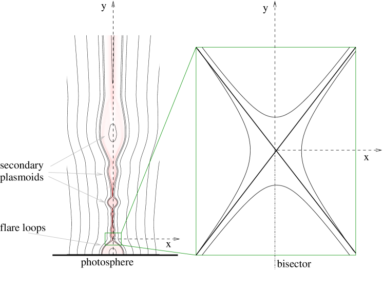
Figure 1.: Scenario of a flare loop with an X-point.bild0

The current density is

$$\vec{\nabla}\times\vec{B}=-\Delta A\,\vec{e}_{z}=\mu_{0}j_{z}\,\vec{e}_{z}\,,\ilabel{1}$$ (3)

such that

$$\vec{\rm B}=\left(\begin{array}[]{cc}B_{11}&B_{12}\\ B_{21}&B_{22}\\ \end{array}\right)\left(\begin{array}[]{c}x\\ y\\ \end{array}\right)\equiv\left(\begin{array}[]{cc}0&2b\\ -2a&0\\ \end{array}\right)\left(\begin{array}[]{c}x\\ y\\ \end{array}\right)\,.\\ \ilabel{1b}$$ (4)

The different topologies of 2D vector fields are represented by two independent parameters, the threshold current $j_{t}$, and the Eigenvalues of $\stackrel{{\scriptstyle\leftrightarrow}}{{B}}$, the $\lambda_{B}$’s, or $j_{z}$, the current in $z$–direction

$$\lambda_{B}=\pm\frac{\mu_{0}}{2}\sqrt{j_{t}^{2}-j_{z}^{2}}\,,\ilabel{1c}$$ (5)

implying a bijective relation between the variables $a$ and $b$ and the threshold $j_{t}$ and the actual current $j_{z}$, to be precise

$$a=-\frac{\mu_{0}}{4}\left(j_{t}+j_{z}\right)\quad b=\frac{\mu_{0}}{4}\left(j_{t}-j_{z}\right)$$ (6)

$$\Leftrightarrow j_{z}=-\frac{2}{\mu_{0}}\left(a+b\right)\quad j_{t}=\frac{2}{\mu_{0}}\left(b-a\right)\,.$$ (7)

We will use the four variables $a,b,j_{t},j_{z}$ if it is convenient, i.e. combinations of the four to simplify the corresponding terms in the equations.

The Eigenvalue $\lambda_{B}$ determines the topological structure of the field and the geometrical shape of the field lines. For a divergence free case there are only three main types of such fields:

• the case that the Eigenvalue is zero ($|j_{t}|=|j_{z}|$) corresponds to the one-dimensional current sheet (degenerated case).

• the case that $|j_{t}|<|j_{z}|$ corresponds to field lines being topological circles (geometrical ellipses), if $j_{t}=0$ ($a=b$), then geometrical circles. All the cases mentioned in the last sentence are so called O-points.

• the case of the so called X-points, where $|j_{t}|>|j_{z}|$.

Only for the case in the last item a magnetic separatrices exist. Such separating field lines must exist to enable magnetic reconnection. A necessary condition for magnetic reconnection in 2D is that the plasma flow crosses magnetic separatrices, see, e.g.,priestforbes,vasyliunas,cowley, sonnerup1, orsonnerup2. The current free case is given by $j_{z}=0$, i.e. $a=-b$ and should be excluded, as dissipation in such a case would have nothing to do with the electric current.

2.2 The basic resistive MHD equations and assumptions

The following analysis is restricted to pure resistive dynamics, i.e. Ohmic heating/dissipation without any other loss terms like viscosity or heat conduction. We choose the coordinate system in such a way, that the gravity is directed in negative $y$-direction (the unit vector in $y$-direction is $\vec{e}_{y}$). The basic resistive stationary MHD equations in 2D are given by (following, e.g., goedbloed)

$$\vec{\nabla}\cdot(\rho\vec{\rm v}) = 0\,,$$ (8)

$$\rho(\vec{\rm v}\cdot\vec{\nabla})\vec{\rm v} = \vec{j}\times\vec{B}-\vec{\nabla}p-\rho g\vec{e}_{y}\,\,,\,g>0$$ (9)

$$E_{0}+{\rm v}_{x}B_{y}-{\rm v}_{y}B_{x} = \eta j_{z}\,,$$ (10)

$$\gamma p\vec{\nabla}\cdot\vec{\rm v}+\vec{\rm v}\cdot\vec{\nabla}p = (\gamma-1)\eta j_{z}^{2}\,,$$ (11)

$$\vec{\nabla}\times\vec{B} = \mu_{0}\vec{j},$$ (12)

$$\vec{\nabla}\cdot\vec{B} = 0\,.$$ (13)

Due to stationary Maxwell equations the electric field in the 2D case has to be constant, i.e. $E_{z}\equiv E_{0}=$const see, e.g., titov2. The same shape of the equations occur, if we introduce a generalized non-ideal term on the right-hand side of Ohm’s law. As the current density is constant close to the X-point (see Eq. 1b), the shape of an effective resistivity is that of the non-idealness $\vec{R}$ (where only the $z$-component is non-zero), writing

$$\vec{\nabla}\cdot(\rho\vec{\rm v}) = 0\,,$$ (14)

$$\rho(\vec{\rm v}\cdot\vec{\nabla})\vec{\rm v} = \vec{j}\times\vec{B}-\vec{\nabla}p-\rho g\vec{e}_{y}\,\,,\,g>0$$ (15)

$$E_{0}+{\rm v}_{x}B_{y}-{\rm v}_{y}B_{x} = \vec{R}\cdot\vec{e}_{z}=R_{z}\,,$$ (16)

$$\gamma p\vec{\nabla}\cdot\vec{\rm v}+\vec{\rm v}\cdot\vec{\nabla}p = (\gamma-1)R_{z}j_{z}\,,$$ (17)

$$\vec{\nabla}\times\vec{B} = \mu_{0}\vec{j},$$ (18)

$$\vec{\nabla}\cdot\vec{B} = 0\,.$$ (19)

The implication is that $\eta=\eta_{\rm effective}\propto R_{z}$, as $j_{z}\neq 0$ is constant close to the null point. The non-idealness resulting from two-fluid approach can be written for the one fluid approach, e.g., followingbraginsky$\!\!x$, as

$$\vec{R}=\eta\vec{j}+\frac{1}{ne}\left(\vec{j}\times\vec{B}-\vec{\nabla}\cdot\stackrel{{\scriptstyle\leftrightarrow}}{{p_{e}}}\right)+\frac{m_{e}}{ne^{2}}\displaystyle\left(\displaystyle\langle\frac{\partial\vec{j}}{\partial t}\rangle_{t}+\vec{\nabla}\cdot\left(\vec{\rm v}\vec{j}+\vec{j}\vec{\rm v}\right)\right)\,,$$ (20)

where $n$ is the particle density, $e$ the absolute value of the electron charge, $\vec{j}\times\vec{B}$ the Hall term, $\stackrel{{\scriptstyle\leftrightarrow}}{{p_{e}}}$ the anisotropic electron pressure tensor, $\frac{\partial\vec{j}}{\partial t}$ the electron acceleration term (in our case averaged over a ‘fitting’  characteristic time scale, as our approach is quasi-stationary), and the tensor divergence $\vec{\nabla}\cdot\left(\vec{\rm v}\vec{j}+\vec{j}\vec{\rm v}\right)$ describes the influence of electron inertia. But even this two-fluid model does not include all terms which may be (additionally) responsible for ‘anomalous’ resistivity or non-idealness, like, e.g., electron scattering by wave turbulence generated due to the Buneman instability (often considered, e.g., buechner and karlicky), ionization-recombination terms, non-linear electron-ion momentum transfer terms, electron and ion viscosities, radiative losses/gains, and so on. As we do not specify the non-idealness, having introduced the effective resistivity, our analysis can be used for all physical models with different types of non-ideal terms. For a more specific view but for non-local models of reconnection with a generalized Ohm’s law, see, e.g.,craigwatson. The term $R$ is therefore only a necessary ‘trigger’ enabling reconnection, not a sufficient one, see, e.g., ks.

We will calculate the (almost) complete solution space of the resistive (non-ideal) MHD close to the null points of flow field and magnetic field. The aim is to find the general correlation between the Jacobians of the plasma velocity and the magnetic field, and the shape of the unspecified non-idealness. At first both vector fields are treated as completely linear, i.e. unbounded fields in an unbounded domain, see section clf. This does not exclude the possibility that in a bounded domain the fields at the boundary are maybe not analytic, but the extrapolation of the field may produce reasonable finite and regular solutions.

In section coli we concentrate on the linearized fields and take only first order terms of the spatial variables into account. A similar method to determine the structure of the non-ideal term and the flow and the magnetic field has been proposed and done, but for the case $j_{z}=0$ and for ‘global’ fields, in the frame of a toy model innifa.

With this linear or linearized fields we can draw conclusions with respect to the other MHD quantities, like pressure, density and resistivity: The lowest order of the magnetic field is linear, the current density is constant, and therefore the Lorentz force $\vec{j}\times\vec{B}$ is linear in $x$ and $y$. This is the reason that all other terms should be also at (the) most of first order in the spatial variables. This leads to the conclusion that the plasma pressure $p$ is at highest order quadratic in $x$ and $y$, to allow for a ‘linear’ pressure force, i.e. we can express $p$ by

$$p=p_{0}+p_{1}x+p_{2}y+p_{3}xy+p_{4}x^{2}+p_{5}y^{2}\,,$$ (21)

where $p_{0}$ to $p_{5}$ are constant coefficients.

As the velocity close to the stagnation point can be represented as a linear term in $x$ and $y$, the $\vec{\rm v}\cdot\vec{\nabla}\vec{\rm v}$ term is also linear in $x$ and $y$, or constant. The mass continuity equation, Eq. (4) implies therefore that the mass density, $\rho$, has to be constant in lowest order close to the stagnation point.

Of course $\rho$ could be a simple linear function close to the null point but that would imply that the mass density has to vanish on a surface, or rather straight line in 2D, depending on the gradient of the density. This null-line could be somewhere inside the ‘linear’ region. In one direction the density could then become negative. We assume that the density $\rho$ is constant in the vicinity of the null points of magnetic and flow field to prevent $\rho$ to have a negative or zero value within the domain of interest. In addition it is a reasonable assumption that close to a stagnation point there is a ‘stagnation region’ , i.e. the density has a maximum or minimum close to the stagnation point.

In the case of completely linear fields it is now evident that the mass continuity equation requires a divergence free velocity field, if we assume all terms to have the same or comparable orders in $x$ and $y$.

One has also to take into consideration that at the magnetic null point $E_{0}$ equals $\eta j_{z}$ and if we assume that the resistivity is constant, then $E_{0}=\eta j_{z}$ everywhere in the vicinity of the neutral point. The same holds for special cases of non-constant resistivity, e.g., if $\eta$ is a function of the current density $j_{z}$ only, one can conclude that in the case of a linear field or in the vicinity of the null point the current density is constant and therefore also the function $\eta=$const, as $\eta=\eta(j_{z}=const)=$const .

The electric field $E_{0}$ is constant also outside the linear region, but the resistivity and current density are, of course, not constant there. This implies that the term ${\rm v}_{x}B_{y}-{\rm v}_{y}B_{x}$ equals to zero within the linear region and therefore the flow is field-aligned everywhere within this region in lowest order of the spatial variables. To get not such ‘trivial’ solutions, which are non-reconnective in lowest order, we have to regard the resistive Ohm’s law as a definition equation for the spatially dependent resistivity, i.e. $\eta=\eta(x,y)$. Therefore, to enable reconnection in the vicinity of the null point, the resistivity cannot be a function of the current density only. We designate and regard this coefficient as an ‘effective’ resistivity or short resistivity, even if this coefficient originates from collisional theory. As the current density is constant inside within the region of the linear field approximation, the (effective) resistivity is a substitute expression for a general non-ideal term, determining, but vice versa also determined by, the flow and magnetic field line structure! This relation between the velocity or flow field $\vec{\rm v}$, the magnetic field $\vec{B}$ and the resistivity $\eta$ will be analysed in this article.

One can also recognize that Eq. (7) (together with the incompressibility) at the stagnation point would require a vanishing resistivity in the absence of additional dissipation terms. Written with all coefficients and comparing with all orders of $x$ and $y$ we get the following system of equations, first from the Euler or momentum equation

$$\rho\left(V_{11}^{2}+V_{12}V_{21}\right)+2p_{4}-2aj_{z} = 0\,,$$ (22)

$$\rho\left(V_{11}^{2}+V_{12}V_{21}\right)+2p_{5}-2bj_{z} = 0\,,$$ (23)

$$p_{3} = 0\,,$$ (24)

$$\rho(V_{21}-V_{21})V_{11}x_{0}-\rho(V_{12}V_{21}+V_{11}^{2})y_{0}+p_{2}+\rho g = 0\,,$$ (25)

$$-\rho V_{11}^{2}x_{0}-\rho V_{12}V_{21}x_{0}+p_{1} = 0\,,$$ (26)

and the equations from the energy equation, first neglecting source or heating terms, only including Ohmic heating,

$$(-V_{11}p_{1}-V_{21}p_{2})x_{0}+(V_{11}p_{2}-V_{12}p_{1})y_{0} = qE_{0}\,,$$ (27)

$$V_{21}p_{2}+V_{11}\left(p_{1}-2x_{0}p_{4}\right)-2V_{12}y_{0}p_{4} = 2aq(V_{11}x_{0}+V_{12}y_{0})$$ (28)

$$V_{12}p_{1}-2V_{21}x_{0}p_{5}+V_{11}\left(2y_{0}p_{5}-p_{2}\right) = 2bq\left(V_{21}x_{0}-V_{11}y_{0}\right)$$ (29)

$$2V_{12}p_{4}+2V_{21}p_{5} = q(-2aV_{12}-2bV_{21})\,,$$ (30)

$$2p_{4}V_{11} = -2aqV_{11}\,,$$ (31)

$$-2p_{5}V_{11} = 2bqV_{11}\,,$$ (32)

where $q:=(\gamma-1)j_{z}$. The equations above are ordered after their physical meaning, the first five equations Eqs. (9) - (13) correspond to the first order momentum equations, while Eqs. (14) - (19) represent the terms of the energy equation. The Eqs. (12), (13) and (14) are of zeroth order in $x$ and $y$. The Eqs. (9), (10), (15) and (16) are of first order in $x$ and $y$, the Eq. (17) is of the order $xy$ and Eq. (18) of second order in $x$, respectively Eqs. (19) is of second order in $y$.

3 Results

In the first subsection we concentrate on linear fields, i.e. fields that are unbounded in an unbounded domain. In the second subsection we take only zero and first order terms of $x$ and $y$ into account, i.e. we regard a Taylor expansion of maximum order one.

3.1 Completely linear fields

clf

If $V_{11}\neq 0$ then from Eqs.(18) and (19) it follows

$$p_{4} = -qa\,$$ (33)

$$p_{5} = -qb\,,$$ (34)

and with two terms of the momentum equation, namely Eq. (9) and Eq. (10), excluding the current free case $j_{z}=0$, i.e. $a=-b$ and the case with O-points, i.e. $a=b$, we infer that

$$\rho(V_{11}^{2}+V_{12}V_{21})=2qa+2aj_{z}\,,$$ (35)

$$\rho(V_{11}^{2}+V_{12}V_{21})=2qb+2bj_{z}\,,$$ (36)

thus $q=(\gamma-1)j_{z}=-j_{z}$ should be valid, leading to $\gamma=0$. As $\gamma=0$ is not representing a realistic equation of state, $V_{11}$ must be zero, taking terms of every order into acount.

This is unaffected by the neglecting other source terms, not mentioned here, as the interesting heat conduction term is of the order zero in $x$ and $y$, and therefore affecting the Eq. (14) only.

Now we use the assumption that $V_{11}=0$. Then we rewrite the MHD equations:

$$\rho V_{12}V_{21}+2p_{4}-2aj_{z} = 0\,,$$

$$\rho V_{12}V_{21}+2p_{5}-2bj_{z} = 0\,,$$

$$-\rho V_{12}V_{21}y_{0}+p_{2}+\rho g = 0\,,$$

$$-\rho V_{12}V_{21}x_{0}+p_{1} = 0\,,$$

$$-V_{12}y_{0}p_{1}-V_{21}x_{0}p_{2} = qE_{0}\,,$$

$$V_{21}p_{2}-2V_{12}y_{0}p_{4} = 2qV_{12}ay_{0}\,,$$

$$V_{12}p_{1}-2V_{21}x_{0}p_{5} = 2qV_{21}bx_{0}\,,$$

$$V_{12}\left(p_{4}+qa\right)+V_{21}\left(p_{5}+qb\right) = 0\,.$$ (37)

With Eqs. (6) and (7) it can clearly be recognized that at the stagnation point the resistivity must be zero. As the electric field $E_{0}$ is constant and $E_{0}=\eta j_{z}$ at the magnetic null point and the stagnation point, we conclude that the electric field is zero (everywhere). The effect of a vanishing compressibility is in resistive MHD also connected with a vanishing electric field.

In addition, as the $x$-offset $x_{0}$ in the fourth equation (a zeroth order term of the force) of the system (24) couples an additional pressure gradient in $x$-direction to this offset only, this offset can be set to zero without loss of generality. Therefore, from $x_{0}=0$ and $E_{0}=0$ we infer $p_{1}=0$, see the fourth and fifth equation of the system (24) (part of the energy/entropy equation).

If we would further allow $y_{0}=0$ in the case of non-vanishing gravity, then there would exist only static solutions either (as in this case $V_{21}$ must be zero it implies that $V_{12}=0$), or the other possible solution branch would need an adiabatic exponent $\gamma=0$.

For the non-degenerated case ($y_{0}\neq 0$) the general solution for the system (24) has two branches:

$$p_{2} = -\frac{\rho g}{2}-\frac{\rho^{2}gV_{12}^{2}}{4b\gamma j_{z}}\mp\frac{\rho g}{4b\gamma j_{z}}\,\sqrt{D}\,,$$

$$p_{4} = \frac{1}{2}\left(\left(2a-b\gamma\right)j_{z}+\frac{\rho V_{12}^{2}}{2}\pm\frac{1}{2}\,\sqrt{D}\right)\,$$

$$p_{5} = \frac{1}{2}\left(\left(2-\gamma\right)bj_{z}+\frac{\rho V_{12}^{2}}{2}\pm\frac{1}{2}\sqrt{D}\right)\,,$$

$$y_{0} = \frac{\rho g}{2b\gamma j_{z}}\,,$$

$$V_{21} = \frac{2\gamma bj_{z}-\rho V_{12}^{2}\mp\sqrt{D}}{2\rho V_{12}}\,,$$ (38)

where the discriminant $D$ must fulfill

$$D=8a\rho V_{12}^{2}\gamma j_{z}+\left(2b\gamma j_{z}-\rho V_{12}^{2}\right)^{2}\geq 0\,$$ (39)

to guarantee that $V_{21}$ is real. This leads to

$$D=\left(\rho V_{12}^{2}\right)^{2}+\left(8a-4b\right)\gamma j_{z}\rho V_{12}^{2}+4b^{2}\gamma^{2}j_{z}^{2}\geq 0$$ (40)

$$\Rightarrow D_{2}:=\left[\left(4a-2b\right)\gamma j_{z}\right]^{2}-4b^{2}\gamma^{2}j_{z}^{2}\geq 0\,,$$ (41)

where $D_{2}$ is the discriminant of the quadratic equation Eq. (27). The inequality Eq. (28) guarantees a real value of $\rho V_{12}^{2}$. That leads together with the convention $j_{t}>0$

$$\left(a-b\right)a\leq 0\quad\Leftrightarrow\quad j_{z}\geq-j_{t}\,.$$ (42)

This implies that either the actual current density $j_{z}\geq 0$, then the field lines are hyperbolas or topological circles, or $j_{z}<0$, then only hyperbolic field lines or (anti-)parallel are possible.

Let us now estimate the influence of the offset in $y$-direction on the solution, e.g., for the situation in the corona. We can express the offset in $y$-direction by using the equation for the offset $y_{0}$ in Eq. (25)

$$y_{0}=\frac{6\rho g}{5\mu_{0}\left(j_{t}/j_{z}-1\right)j_{z}^{2}}\,,$$ (43)

assuming that $\gamma=5/3$.

We demand that the configuration should really be an X-point, but not a one-dimensional sheet, therefore we assume that the relation between the two characteristic currents is given by a value not much larger than $j_{z}/j_{t}\approx 0.999$ (correponds to an opening angle of the smaller separatrix angle of only about 2 degrees). With the electron charge $e$, the number density $n$ and the drift velocity ${\rm v}_{d}$ and $j_{z}=ne{\rm v}_{d}$, it follows for $y_{0}$

$$y_{0}=1200\,\frac{\rho g}{\mu_{0}j_{z}^{2}}=1.2\times 10^{3}\,\frac{nm_{p}g}{\mu_{0}n^{2}e^{2}{\rm v}_{d}^{2}}$$ (44)

The value $|y_{0}|$ must now be compared with the typical lengthscale and values of a magnetic field close to a null point, i.e. the coronal magnetic field is about $B_{c}\approx 10^{-2}T$ (the index ‘c’ stands for ‘coronal’) and the scale on which the magnetic field varies linearly should be larger than a Debye length (for coronal parameters in the range of mm to cm) , but much smaller than the active region loops ($l_{c}\approx 10^{7.5}$m) to get an upper limit for $|y_{0}|$. We therefore use the approximate current sheet thickness $d$. To estimate the current sheet thickness of a finite current sheet, we assume again that the current density $j_{z}=ne{\rm v}_{d}$, where ${\rm v}_{d}$ is the drift velocity, which should not exceed the thermal velocity (of the electrons), i.e. ${\rm v}_{d}\leq\sqrt{3k_{B}T/m_{e}}$. Let $k_{B}=1.38\times 10^{-23}$JK^-1 the Boltzmann constant, $\varepsilon_{0}=8.85\times 10^{-12}$A²s⁴kg^-1m^-3 the dielectric constant, $m_{p}=1.67\times 10^{-27}$kg the mass of the proton, $m_{e}=9.1\times 10^{-31}$kg the mass of the electron, $n=1.6\times 10^{14}$m³ the number density, and $T_{d}=10^{6}$K (as the thermal temperature is about $T=2\times 10^{6}$K, we consider an effective temperature $T_{d}$, thus that the corresponding drift velocity ${\rm v}_{d}$ is definitely below the critical drift velocity given by temperature ${\rm v}_{th}^{2}=3k_{B}T/m_{e}$ to guarantee a stable stationary current, instead of an kinetic instability see, e.g., papadopoulos) the approximate temperature (for the coronal parameters see, e.g., stix). We choose a ‘small’ current density to get the upper limit of $y_{0}$. The offset is then given by

$$|y_{0}|=\frac{1.2\times 10^{3}m_{p}g}{\mu_{0}ne^{2}{\rm v}_{d}^{2}}=\frac{1.2\times 10^{3}\,m_{p}g}{\mu_{0}ne^{2}\left(\!\sqrt{3k_{B}T_{d}/m_{e}}\right)^{2}}\approx 3\times 10^{-6}{\rm m}\,.$$ (45)

The lower bound of the current sheet thickness is approximately given by

$$d\approx\frac{B_{c}}{\mu_{0}j_{z}}=\frac{B_{c}}{\mu_{0}ne\sqrt{3k_{B}T_{d}/m_{e}}}\approx 33{\rm m}\,.$$ (46)

The fraction of both values should be $y_{0}/d\ll 1$and is then determined by

$$\frac{y_{0}}{d}=1.2\times 10^{3}\,\frac{m_{p}g}{e{\rm v}_{d}B_{c}}=\frac{1.2\times 10^{3}\,m_{p}g}{e\sqrt{3k_{B}T_{d}/m_{e}}B_{c}}\approx 6\times 10^{-8}\ll 1\,.$$ (47)

Thus for typical coronal parameters the offset in $y$-direction has a value of about mm or even some orders of magnitude less, in contrast to the value of the typical lengthscale of the linear X-point region which is at least of the order of one meter or some tenth of meters or even more. This is an argument or rough justification to neglect the term of the interaction between the shift and the second derivative of $\vec{\rm v}$.

Even if we assume that the drift velocity ${\rm v}_{d}$ is, let us say six orders, smaller than the thermal velocity, the fraction $|y_{0}|/d$ would be of the order of some percent. Therefore, even in this extreme regime of the drift velocity, the stagnation point is located within the current sheet, assuming that the sheet is really two-dimensional (non-singular) and its extensions in both coordinate directions are about of the same order. The complete mentioned discussion is valid exactly only in the case of unbounded fields, but it shows that in general the offset due to gravity can be neglected.

3.1.1 Discussion of the discriminant $D$

The discriminant $D_{2}$ in Eq. (28), being larger than zero is only a necessary criterion. That $\rho V_{12}^{2}>0$ has also to be guaranteed.

To fullfil the relation $D\geq 0$ we define two values, namely

$$\epsilon_{1}:=\rho V_{12,crit1}^{2} = \frac{\mu_{0}}{2}\left(3j_{t}+j_{z}\right)\gamma j_{z}+2\mu_{0}\gamma|j_{z}|\sqrt{\frac{j_{t}\left(j_{t}+j_{z}\right)}{2}}$$ (48)

$$\epsilon_{2}:=\rho V_{12,crit2}^{2} = \frac{\mu_{0}}{2}\left(3j_{t}+j_{z}\right)\gamma j_{z}-2\mu_{0}\gamma|j_{z}|\sqrt{\frac{j_{t}\left(j_{t}+j_{z}\right)}{2}}$$ (49)

to represent the relation Eq. (27)

$$\left(\rho V_{12}^{2}-\epsilon_{1}\right)\left(\rho V_{12}^{2}-\epsilon_{2}\right)\geq 0$$ (50)

$$\Rightarrow\quad\textrm{C(ase)I} \rho V_{12}^{2}\geq\epsilon_{1}\quad\land\quad\rho V_{12}^{2}\geq\epsilon_{2}$$ (51)

is valid or

$$\Rightarrow\quad\textrm{C(ase)II} \rho V_{12}^{2}\leq\epsilon_{1}\quad\land\quad\rho V_{12}^{2}\leq\epsilon_{2}\,,$$ (52)

which implies for CI $\rho V_{12}^{2}\geq{\rm max}(\epsilon_{1},\epsilon_{2})=\epsilon_{1}$ and for CII $\rho V_{12}^{2}\leq{\rm min}(\epsilon_{1},\epsilon_{2})=\epsilon_{2}$. The values $\epsilon_{1,2}$ are explicit functions of the current densities $j_{t}$ and $j_{z}$. This gives us restrictions for $V_{12}$: for $j_{z}\geq 0$ the lower bound for $V_{12}$ is given by the left relation of Eq. (31) otherwise the lower bound is zero, writing

$$\rho V_{12}^{2} \geq \frac{\mu_{0}}{2}\left(3j_{t}+j_{z}\right)\gamma j_{z}+2\mu_{0}\gamma|j_{z}|\sqrt{\frac{j_{t}\left(j_{t}+j_{z}\right)}{2}}\,,$$ (53)

such that the non-admissible region is then given by

$$V_{12}\not\in\left[+V_{12,crit1},-V_{12,crit1}\right]\,,$$ (54)

and $V_{12,crit1}$ is given by

$$V_{12,crit1}=\sqrt{\frac{\frac{\mu_{0}}{2}\left(3j_{t}+j_{z}\right)\gamma j_{z}+2\mu_{0}\gamma|j_{z}|\sqrt{\frac{j_{t}\left(j_{t}+j_{z}\right)}{2}}}{\rho}}\,.$$ (55)

For $j_{z}\leq 0$ all values of $V_{12}$ are allowed. There are no restrictions for $V_{12}$, as for $j_{z}=0$ the critical value $V_{12,crit1}=0$ and for $j_{z}<0$ all values of $V_{12,crit1}$ are imaginary.

For CII it is clear that the criterion is given by

$$\rho V_{12}^{2} \leq \frac{\mu_{0}}{2}\left(3j_{t}+j_{z}\right)\gamma j_{z}-2\mu_{0}\gamma|j_{z}|\sqrt{\frac{j_{t}\left(j_{t}+j_{z}\right)}{2}}\,.$$ (56)

For $j_{z}<0$ no value of $V_{12}$ can satisfy the relation Eq. (35). Only for $j_{z}\geq 0$ solutions exist in the region beyond the curve Fig. bild and the $j_{z}$-axis.

Thus we can summarize: For $j_{z}\geq 0$ the allowed values for $\rho V_{12}$ are given by the relation

$$\epsilon_{2}\geq\rho V_{12}^{2}\geq 0\quad\lor\quad\rho V_{12}^{2}\geq\epsilon_{1}\,.$$ (57)

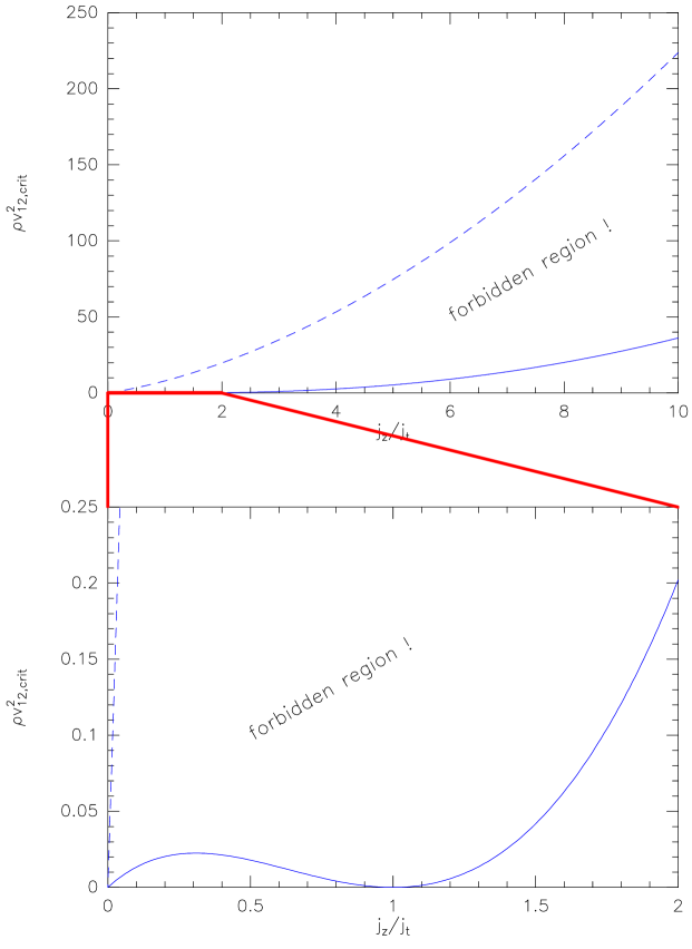
Figure 2.: Not all values for the ‘free’ velocity parameter $V_{12}$ are allowed. There exist some forbidden regions for the velocity parameter.bild

3.1.2 Solutions with shear flows

In the case of a vanishing $V_{12}$ or $V_{21}$ the equations again lead to the statement that either $V_{12}=V_{21}=0$ in both cases or that again $\gamma=0$. This implies that the allowed flows are of higher orders with respect to the spatial variables, like indicated in priest75$\!\!,$ or need special, maybe unphysical thermodynamical constraints. Also the case of general shear flows leads to $\gamma=0$. Such solutions will not be discussed here.

3.1.3 The resistivity

The resistivity is given by the $z$-component of $\vec{\rm v}\times\vec{B}$ and results in the quadric

$$\eta=\frac{1}{j_{z}}\left(2aV_{12}y_{0}x-\left(2aV_{12}+2bV_{21}\right)xy\right)\,.$$ (58)

Neglecting the term with $y_{0}$, the above equation shows that the isocontours of the resistivity have four branches. In two quadrants $\eta$ has a positive sign and the other two quadrants represent an effective negative resistivity.

This example of unbounded fields shows an interesting behaviour because the solutions are exact analytical ones and they exhibit the fact that there is a special relation between the derivatives of $\vec{\rm v}$ and of $\vec{B}$ connected about algebraic varieties which generate the solutions. We stop these investigations here due to the problem of negative resistivity. To interpret this negative effective resistivity (or negative non-idealness) and search for a reasonable physical interpretation or correponding physical mechanism needs further investigation.

3.2 Complete linearization of the resistive system concerning $x$ and $y$

coli Here $V_{11}\neq 0$ in general, as the equation which contradicts the thermodynamical constraints, the last two equations of Eqs. (18) and  (19), being part of the energy equation, are neglected due to their higher order in $x,y$.

In this case we only need to regard equations, being of first order in $x$ and $y$, namely

$$\rho\left(V_{11}^{2}+V_{12}V_{21}\right)+2p_{4}-2aj_{z} = 0\,,$$ (59)

$$\rho\left(V_{11}^{2}+V_{12}V_{21}\right)+2p_{5}-2bj_{z} = 0\,,$$ (60)

$$p_{3} = 0\,,$$ (61)

$$-\rho(V_{12}V_{21}+V_{11}^{2})y_{0}+p_{2}+\rho g = 0\,,$$ (62)

$$-\rho V_{11}^{2}x_{0}-\rho V_{12}V_{21}x_{0}+p_{1} = 0\,,$$ (63)

$$(-V_{11}p_{1}-V_{21}p_{2})x_{0}+(V_{11}p_{2}-V_{12}p_{1})y_{0} = 0\,,$$ (64)

$$V_{21}p_{2}+V_{11}\left(p_{1}-2x_{0}p_{4}\right)-2V_{12}y_{0}p_{4} = 2aq(V_{11}x_{0}+V_{12}y_{0})\,,$$ (65)

$$V_{12}p_{1}-2V_{21}x_{0}p_{5}+V_{11}\left(2y_{0}p_{5}-p_{2}\right) = 2bq\left(V_{21}x_{0}-V_{11}y_{0}\right)\,,$$ (66)

which contain only terms of first order. This is a nonlinear system consisting of eight, but, of course, effectively seven equations for nine unknowns.

3.3 Solutions without gravity and shift

sws

In this case the stagnation point is identical with the magnetic null point. The general solutions is now represented by

$$p_{4} = -\frac{\rho}{2}\left(V_{11}^{2}+V_{12}V_{21}\right)+aj_{z}$$

$$p_{5} = -\frac{\rho}{2}\left(V_{11}^{2}+V_{12}V_{21}\right)+bj_{z}\,,$$ (67)

with free parameters $V_{11}$ and $V_{12}$ (and, of course, the ‘magnetic parameters’ the threshold current $j_{t}$ and the actual current $j_{z}$). The parameter $V_{21}$ is not free, as it is determined by the fact that the quadric (surface), representing the resistivity, must be an elliptic paraboloid. We have to introduce another parameter $s$ to express $V_{21}$ as function of $V_{12}$ and $s$. The elliptic paraboloid is the only quadric that allows a positive resistivity with one zero (the vertex of the paraboloid) at the magnetic null point. All other quadrics can be excluded, with the exception of the degenerated case of a cylindrical paraboloid, see, e.g.,bronstein or bartsch. The cylindrical paraboloids are limiting cases with $s=\pm 1$ as is shown as in the example in Fig. cross4 (here the specific value is $s=-1$). The general solution is then parameterized by $V_{11},V_{12},s$

$$V_{21}=\frac{j_{t}+j_{z}}{j_{t}-j_{z}}V_{12}+2sV_{11}\,\frac{\sqrt{j_{t}^{2}-j_{z}^{2}}}{j_{t}-j_{z}}\,,$$ (68)

with the restriction $s\in[-1,1]$. Multiplication of Eq. (cl16) with $V_{12}$, inserting this expression into the expression for the Eigenvalue $\lambda_{V}^{2}=V_{11}^{2}+V_{12}V_{21}$, and completing the square gives

$$\lambda_{V}^{2} = V_{11}^{2}+V_{12}V_{21}$$ (69)

$$= \left(V_{11}+sV_{12}\frac{\sqrt{j_{t}^{2}-j_{z}^{2}}}{j_{t}-j_{z}}\right)^{2}+\left(1-s^{2}\right)V_{12}^{2}\frac{j_{t}+j_{z}}{j_{t}-j_{z}}\geq 0\,.$$

If $|j_{z}|<j_{t}$ and $|s|<1$ as assumed, the magnetic field is of hyperbolic type and it is guaranteed that the stagnation point is also of hyperbolic type, i.e. has two purely real Eigenvalues, namely one positive value and a negative counterpart.

Although the solutions shown here are no reconnection solutions, as the electric field has to be zero, because only resistive dissipation is included in our investigation, they represent almost reconnection solutions(=reconnection-like solutions) where the necessary condition for reconnection is fulfilled.

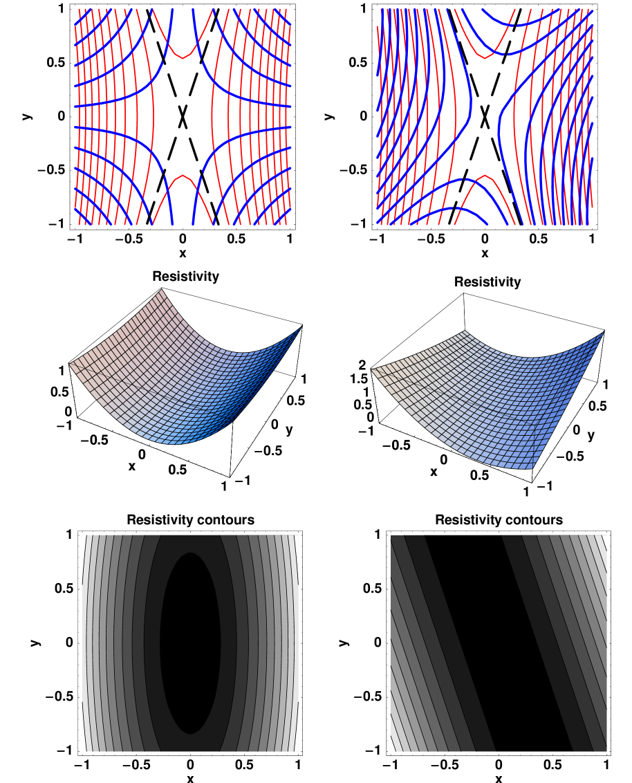
Figure 3.: Flow for the parameters $V_{11}=V_{12}=1$ and $s=0$ (left column) and $s=-1$ (right column), crossing all four magnetic separatrix branches (top panels), shape of the positive resistivity (middle panels), and the elliptic shaped contours of the resistivity (bottom panels).cross4

Let us investigate now the geometry, respectively the slopes of the separatrices of the flow and the magnetic field. Defining $J_{z}:=j_{z}/j_{t}$, the magnetic separatrix is given by $A=0$ and $A=\frac{\mu_{0}}{4}\left[\left(j_{t}-j_{z})y^{2}-\left(j_{t}+j_{z}\right)x^{2}\right)\right]$ (we restrict this to $|J_{z}|<1$) and can therefore be expressed by

$$\sqrt{1-J_{z}}\,y\pm\sqrt{1+J_{z}}\,x=0\,\,\Leftrightarrow\,\,y=\pm\frac{\sqrt{1+J_{z}}}{\sqrt{1-J_{z}}}x:=\pm K_{m}x\,,$$ (70)

where $\pm K_{m}$ is the slope of the both magnetic separatrix lines or to say the both asymptotes. As $V_{21}$ is given by the general solution, Eq. (cl16), by defining a stream function $\psi$ via

$${\rm v}_{x}=\frac{\partial\psi}{\partial y}\quad\textrm{and}\quad{\rm v}_{y}=-\frac{\partial\psi}{\partial x}\,,$$ (71)

we can integrate the above equations and get for the stream function

$$\psi=\frac{V_{12}^{2}}{2}y^{2}-\frac{V_{21}^{2}}{2}x^{2}+V_{11}xy\,.$$ (72)

The fluid separatrix is here given by $\psi=0$, geometrically this are asymtotical lines (asymptotes).

We will briefly discuss the problem that the magnetic separatrix is partially identical with the hydrodynamic separatrix. In this case the plasma flow can only take place across one part of the separatrix, or both separatrix lines are identical and no reconnection can take place.

One can clearly recognize that in the case $V_{11}=0$ and thus $(V_{21}/V_{12})^{2}=(1+J_{z})/(1-J_{z})$ both corresponding asymtotical branches($=$separatrix lines) have the same slope. Thus the hydrodynamical separatrix and the magnetic separatrix are identical, the plasma cannot cross the magnetic separatrix and therefore no reconnection can take place.

Writing $y(x)=K_{V}x$ (if $V_{11},V_{12}\neq 0$), where $K_{V}$ is the slope of the hydrodynamic separatrix, and inserting this into $\frac{V_{12}^{2}}{2}y^{2}-\frac{V_{21}^{2}}{2}x^{2}+V_{11}xy=0$ with the parametric expression for $V_{21}$ in Eq. (cl16), we get the slopes $K_{V1,V2}$ of the two asymptotes/separatrix lines

$$K_{V1,2} =-\frac{V_{11}}{V_{12}}\pm\sqrt{\frac{V_{11}^{2}+V_{12}V_{21}}{V_{12}^{2}}}$$ (73)

$$=\frac{-V_{11}\pm\sqrt{V_{11}^{2}+2sV_{11}V_{12}\frac{\sqrt{1-J_{z}^{2}}}{1-J_{z}}+V_{12}^{2}\,\frac{1+J_{z}}{1-J_{z}}}}{V_{12}}$$

$$=-V_{rel}\pm\sqrt{V_{rel}^{2}+2sV_{rel}\frac{\sqrt{1-J_{z}^{2}}}{1-J_{z}}+\frac{1+J_{z}}{1-J_{z}}}\,\,\,\,,$$

where $V_{rel}=V_{11}/V_{12}$. For $V_{12}=0\neq V_{11}$ the asymptotes are given by $x=0$ and $y=s\sqrt{(1+J_{z})/(1-J_{z})}x$, and for $V_{12}=V_{21}=0$ we get $x=0$ and $y=0$ as separatrices.

Let $V_{11}=V_{12}(=1)$, then

$$K_{V1,2}=-1\pm\sqrt{\left(1+s\frac{\sqrt{1-J_{z}^{2}}}{1-J_{z}}\right)^{2}}=-1\pm\left(1+s\frac{\sqrt{1-J_{z}^{2}}}{1-J_{z}}\right)\,\,.$$ (74)

There is one corresponding slope of the flow separatrix with respect to one of the magnetic separatrix lines, if $s=\pm 1$.

Therefore we can formulate the following theorem (in analogy to known anti-reconnection theorems), which is now restricted to almost reconnective solutions with vanishingly small electric fields and resistive disspation only, i.e. vanishing non-resistive dissipation mechanisms:

Theorem

If the flow close to the null point is in good approximation incompressible, the electric field is negligible and other kinds of dissipation mechanisms than the resistive dissipation are also negligible, then the plasma flow cannot cross the magnetic separatrices if for the both slopes of the both magnetic separatrix lines $K_{m}=K_{m1}=-K_{m2}$ with $K_{m}=\sqrt{(1+J_{z})/(1-J_{z})}$ and the following is valid:

$$I.\,\,a)\,K_{m}=K_{V1}\quad\land\quad b)\,-K_{m}=K_{V2}$$

or

$$II.\,\,a)\,K_{m}=K_{V2}\quad\land\quad b)\,-K_{m}=K_{V1}$$ (75)

If only I.a) or I.b) or II.a) or II.b) is valid then only one magnetic separatrix can be crossed and as the other stream lines converge to the second magnetic separatrix line without crossings, one could call this reconnective annihilation, see, e.g., Priest & Forbes (2000). The necessary condition for a complete non-crossing is $V_{11}=0$ for $V_{12}\neq 0$ and for only partly crossing flows $s=\pm 1$.

For almost all values of $s$, here $s=0$, the flow in Fig.cross4 (left column) crosses all four separatrix branches (all two separatrix lines), the resistivity is positive (only zero at the null point, middle panel), and their isocontours are ellipses (bottom panel). For the special parameter $s=-1$ it can be seen in Fig. cross4 (right column) that the flow, like for the aforementioned magnetic reconnective annihilation solutions, crosses only the separatrix line with the positive slope, while it converges to the other magnetic separatrix, being almost field aligned (top panel), the resistivity being also postive (middle panel), and the isocontours of the resistivity are straight lines (bottom panel).

We now focus on the effective resistivity and therefore on the nature of ohmic heating/disspation. The resistivity is given by

$$\eta=\frac{\mu_{0}}{2}\frac{V_{11}}{j_{z}}\left[\left(j_{t}+j_{z}\right)x^{2}-2s\sqrt{j_{t}^{2}-j_{z}^{2}}xy+\left(j_{t}-j_{z}\right)y^{2}\right].$$ (76)

To ensure that the dissipation is positive we prove that the term $\left(j_{t}+j_{z}\right)x^{2}-2s\sqrt{j_{t}^{2}-j_{z}^{2}}xy+\left(j_{t}-j_{z}\right)y^{2}$ is larger than zero (or zero) for all $s$ and $x,y$. Let $K_{1,2}=j_{t}\pm j_{z}$ and $K_{1},K_{2}>0$ as required for an X-point. Then

$$0 \leq\left(\sqrt{K_{1}}x-s\sqrt{K_{2}}y\right)^{2}=K_{1}x^{2}-2s\sqrt{K_{1}K_{2}}xy+s^{2}K_{2}y^{2}$$ (77)

$$\leq K_{1}x^{2}-2s\sqrt{K_{1}K_{2}}xy+K_{2}y^{2}.\quad\square$$

This implies that the sign of the resistivity $\eta$ depends on the sign of $\frac{V_{11}}{j_{z}}$. As the dissipation should be positive, i.e. $\eta>0$, thus $V_{11}$ and $j_{z}$ must have the same sign.

For $s=\pm 1$ it can be recognized from Eq. (resi1) and from the bottom panel Fig. cross4 (for the case $s=-1$) that the resistivity contour lines are straight lines given by $\eta=\mu_{0}V_{11}/(2j_{z})\,(\sqrt{j_{t}+j_{z}}x\pm\sqrt{j_{t}-j_{z}}y)^{2}$, and therefore the resistivity has the structure of a one-dimensional sheet. The case $s=\pm 1$ therefore reflects the 1D character of the non-idealness, which can also be found in the papers of craighenton.

4 Conclusions

We analyse the solution space of the MHD system with a generalized non-idealness in Ohm’s law close to an X-type magnetic null point. This procedure is done to get non-ideal/resistive but formally non-reconnective solutions that can be regarded as reconnection solutions with a vanishing electric field. Such solutions show the parameters and their relation amongst each others, to get non-ideal non-reconnective, i.e. either almost reconnective annihilation or completely almost reconnective (= reconnection-like) solutions.

We assume that the flow close to the magnetic null point is governed strictly by the pure non-ideal/resistive system of MHD equations, and that the stagnation point is close to the null point (or that both singular points in the plane are identical). The focus is on the region close to the magnetic null point to investigate the possible type of topology of the corresponding stagnation point (flow). To use a closure for the equations and to analyse the resistive MHD system we use the corresponding energy equation.

We further assume that the density is constant close to the stagnation point. This assumption is not a necessary, but a plausible condition concerning the mass distribution in the vicinity of stagnation points. This leads to a vanishing divergence of the plasma velocity and as a logical consequence to a vanishing resistivity close to the stagnation point. Inserting this into resistive Ohm’s law implies that the electric field has to vanish at the stagnation point. We conclude that the electric field has to be zero, and as a consequence of the 2D stationary approach the electric field has to be zero everywhere.

This case of vanishing divergence of the velocity field and thus of a vanishing electric field can be regarded as a physical approximation or limit. Obviously a classical reconnection process requires a non-vanishing divergence of the velocity field to produce a non-zero reconnection rate, determined by the constant electric field $E_{0}$, see, e.g.,priestforbes.

From resistive Ohm’s law one can clearly recognize that close to the magnetic null point the electric field is identical to the ‘convective’ electric field generated by the product from resistivity and current density. As the electric field is zero, the resistivity inside the finite current sheet must be zero at the magnetic neutral point. The effect is that the resistivity cannot be constant close to the magnetic neutral point. Therefore the resistive Ohm’s law is an equation determining the topological type of the magnetic field and the velocity field and connecting/relating it to the shape of the resistivity, which is a quadratic function of the spatial coordinates. We call this spatially varying resistivity effective resistivity or for short resistivity as usual. As the current density is constant close to the magnetic null point, the right hand side of Ohm’s law, Eq. (6) could be regarded as a generalized non-ideal term.

A necessary condition for reconnection is that the plasma flow can cross magnetic separatrices. We found that crossing of magnetic separatrices requires also an X-type stagnation point flow if the effective resistivity and thus the dissipation should be positive.

The sufficient criterion for reconnection is the crossing of the separatrix and the non-vanishing electric field. This reconnection process can take place for/in the incompressible case if there is not only a resistive, but an additional non-resistive dissipation (term) that occurs only in the energy equation. Therefore one possibility could be heat conduction. Another possibility is the viscous case with constant viscosity. Here, the Laplacian of the velocity field vanishes in the first order momentum equation of the ions (Navier-Stokes) as the velocity field is linear. These cases have to be investigated in more detail but have been discussed under the assumption of constant resistivity, e.g., by priestforbes.

The analyses started by us here will be extended to configurations that have density gradients close to the stagnation point and therefore allow for a non-zero electric field. The extension to energy equations allowing for a deviation from the classical energy equation of resistive MHD will provide us with a relation between the deviation from pure resistive dissipation and deviation from the classical (X-type) stagnation point flow.

Acknowledgements

D.H. Nickeler acknowledges financial support from GAAV ČR grant No. IAA300030804 and M. Karlický from GA ČR grant No. 300030701. D.H. Nickeler is grateful to Dr. Michaela Kraus for the help in preparing Fig.2 and careful reading of the manuscript.

References

- Amann (1995) Amann, H.: 1995, Gewöhnliche Differentialgleichungen Walter de Gruyter, Berlin.
- Arnold (1990) Arnold, V.: 1992, Ordinary Differential Equations, Springer, Berlin.
- Bartsch (1984) Bartsch, E.: 1984, Mathematische Formeln, VEB Fachbuchverlag, Leipzig.
- Baty, Forbes, and Priest (2009) Baty, H., Forbes, T.G. and Priest, E.R.: 2009, Phys. of Plasmas 16, 012102.
- Braginsky (1965) Braginsky, S.I.: 1965, Rev. Plasma Phys. 1, 205.
- Bronstein and Semendjajew (1987) Bronstein, I.N. , and Semendjajew, K.A.: 1987, Taschenbuch der Mathematik, Verlag Harri Deutsch, Frankfurt/Main.
- Buechner and Elkina (2006) Buechner, J. and Elkina, N.: 2006, Space Sci. Rev. 121, 237.
- Cowley (1976) Cowley, S.W.H.: 1976, J. Geophys. Res. 81, 3455.
- Craig and Henton (1995) Craig, I.J.D. and Henton, S.M.: 1995, ApJ 450, 280.
- Craig and Rickard (1994) Craig, I.J.D. and Rickard, G.J.: 1994, A&A 287, 261.
- Craig and Watson (2003) Craig, I.J.D. and Watson, P.G.: 2003, Sol. Phys. 214, 131.
- Goedbloed and Poedts (2004) Goedbloed, J.P. and Poedts, S.: 2004, Principles of Magnetohydrodynamics, Cambridge University Press, Cambridge.
- Karlický and Bárta (2005) Karlický, M. and Bárta, M.-J.: 2005, Sol. Phys. 247, 335.
- Nickeler and Fahr (2005) Nickeler, D. and Fahr, H.-J.: 2005, Adv. Space Res. 35, 2067.
- Nickeler, Goedbloed, and Fahr (2006) Nickeler, D., Goedbloed, H., and Fahr, H.-J.: 2006, A&A 454, 797.
- Papadopoulos (1977) Papadopoulos, K.:, 1977, Rev. of Geophysics 15, 113.
- Parnell, Neukirch, and Priest (1996) Parnell, C., Neukirch, T., and Priest, E.: 1996, Phys. of Plasmas 3, 759.
- Petschek (1964) Petschek, H.E.: 1964, in W.N. Hess (ed.), The Physics of Solar Flares, AAS-NASA Symp., p. 425.
- Priest and Cowley (1975) Priest, E. and Cowley, S.W.H.: 1975, J. of Plasma Phys. 14(2), 271.
- Priest and Forbes (2000) Priest, E. and Forbes, T.: 2000, Magnetic Reconnection Cambridge University Press, Cambridge.
- Priest et al. (1994) Priest, E., Titov, V.S., Vekstein, G.E., and Rikard, G.J.: 1994, J. Geophys. Res. 99(A11), 21467.
- Reitmann (1990) Reitmann, V.: 1996, Reguläre und chaotische Dynamik, B.G. Teubner Verlagsgesellschaft, Leipzig.
- Schindler, Hesse, and Birn (1988) Schindler, K., Hesse, M., and Birn, J.: 1988, J. Geophys. Res. 93, 5547.
- Sonnerup (1979) Sonnerup, B.U.Ö.: 1979, in L.J. Lanzerotti, C.F. Kennel, and E.N. Parker (eds.) Solar Systems Plasma Physics, Vol.3, North Holland, Amsterdam, p. 45.
- Sonnerup (1984) Sonnerup, B.U.Ö., Baum, P.J., Birn, J., et al.: 1984, in D.M. Butler and K. Papadopoulos (eds.), Solar Terrestrial Physics: Present and Future, NASA, Ref. Publ. Vol. 1120, p. 1.
- Stix (2002) Stix, M.: 2002, The sun, Springer, Berlin/Heidelberg/New York.
- Sweet (1958) Sweet, P.A.: 1958, Nuovo Cimento 8, 188.
- Tassi, Titov, and Hornig (2002) Tassi, E., Titov, V.S., and Hornig, G.: 2002, Phys. Letters A 302, 313.
- Titov and Hornig (2000) Titov, V.S. and Hornig, G.: 2000, Phys. of Plasmas 7, 3542.
- Titov, Tassi, and Hornig (2004) Titov, V.S., Tassi, E., and Hornig, G.: 2004, Phys. of Plasmas 11, 4662.
- Watson and Craig (1998) Watson, P.G., and Craig, I.J.D.: 1998, ApJ 505, 363.
- Vasyliunas (1975) Vasyliunas, V.M.: 1975, Rev. Geophys. 13, 303.