Construction of Coupled Period-Mass Functions in Extrasolar Planets through the Nonparametric Approach

Abstract

Using the period and mass data of two hundred and seventy-nine extrasolar planets, we have constructed a coupled period-mass function through the non-parametric approach. This analytic expression of the coupled period-mass function has been obtained for the first time in this field. Moreover, due to a moderate period-mass correlation, the shapes of mass/period functions vary as a function of period/mass. These results of mass and period functions give way to two important implications: (1) the deficit of massive close-in planets is confirmed, and (2) the more massive planets have larger ranges of possible semi-major axes. These interesting statistical results will provide important clues into the theories of planetary formation.

Key words: extrasolar planets, distribution functions, correlation coefficients

1 Introduction and Motivation

After the first detection of an extra-solar planet (exoplanet) around a millisecond pulsar in 1992 (Wolszczan & Frail 1992), it was soon reported that another exoplanet, the first one around a sun-like star, i.e. 51 Pegasi b, was found (Mayor & Queloz 1995). Ever since then, there has been a continuous flood of discoveries of extra-solar planets. As of February 2008, more than 200 planets have been detected around solar type stars. These discoveries have led to a new era in the study of planetary systems. For example, the traditional theory for the formation of the Solar System does not likely explain certain structures of extra-solar planetary systems. This is due to the properties, discovered in extra-solar planetary systems, being quite unlike our own. Many detailed simulations and mechanisms have been proposed to explore these important issues (Jiang & Ip 2001, Kinoshita & Nakai 2001, Armitage et al. 2002, Ji et al. 2003, Jiang & Yeh 2004a, Jiang & Yeh 2004b, Boss 2005, Jiang & Yeh 2007, Rice et al. 2008).

As the number of detected exoplanets keeps increasing, the statistical properties of exoplanets have become more meaningful. For example, assuming that the mass and period distributions are two independent power-law functions, Tabachnik & Tremaine (2002) used the maximum likelihood method to determine the best power-index. However, the possibility of a mass-period correlation is not addressed in their work. Zucker & Mazeh (2002) determined the correlation coefficient between mass and period in logarithmic space and concluded that the mass-period correlation is significant.

On the other hand, a clustering analysis of the data we have on exoplanets also gives some interesting results. Jiang et al. (2006) took a first step into clustering analysis and found that the mass distribution is continuous, and the orbital population could be classified into three clusters which correspond to the exoplanets in the regimes of tidal, ongoing tidal and disc interaction. Marchi (2007) also worked on clustering through different methods.

To take things a step further from the mass-period distribution function of Tabachnik & Tremaine (2002) and the mass-period correlation of Zucker & Mazeh (2002), Jiang, Yeh, Chang, & Hung (2007) (hereafter JYCH07) employed an algorithm to construct a coupled mass-period function numerically. They were able to include the possible correlation of mass and period into the distribution function for the first time in this field and obtained a distribution function that found a correlation to be consistent. In fact, the mass-period distribution obtained by JYCH07 should be called the mass-period probability density function (pdf) in statistics. The integral of pdf is then called the cumulative distribution function (cdf). We will use the above terms in this paper.

Although JYCH07 successfully constructed the coupled mass-period pdf numerically, due to constraints in the algorithm they employed, they were forced to use the parametric approach of $\beta$-distribution on the pdf fitting. The pdf is a basic characteristic describing the behavior of random variables, i.e. mass and period, and is so important that one has to choose the underlying functional form carefully. One possibility to address this problem is to use the nonparametric approach. This is because the nonparametric approach is a distribution-free inference. That is, an inference that is made without any assumptions regarding the functional form of the underlying distribution. In addition, the most valuable indication of the nonparametric approach is to let the data speak for itself. We therefore see no other reasonable course of action than to use the nonparametric approach in this paper.

Moreover, we still consider the period-mass coupling even while the pdf and cdf are being constructed. In order to make it possible to proceed, we will employ a method called “Copula Modelling” to obtain the coupled pdf and cdf on the period and mass of exoplanets. This method is more general than the one used in JYCH07 so that a nonparametric approach can be used to obtain the coupled pdf. “Copula Modelling” has a long history of development and was too complicated to be used with real data, in practical terms, until Trivedi & Zimmer (2005) clearly demonstrated a standard modelling procedure.

In §2, we briefly describe the data and in §3, an estimation of the nonparametric approach will be done. In §4, we introduce the method of Copula Modelling and demonstrate its credibility. The Copula Modelling will then be directly applied on the data of exoplanets. The results will be described and discussed in §5. Our main conclusions will be found in §6.

2 The Data

We took samples of exoplanets from The Extrasolar Planets Encyclopaedia (http://
exoplanet.eu/catalog-all.php), 2008 April 10. Our samples do not include OGLE235-MOA53b, 2M1207b, GQ Lupb, AB Pic b, SCR 1845b, UScoCTIO108b, or SWEEPS-04 because either their mass or their period data was not listed. The outlier, PSR B1620-26b, with a huge period (100 years), is also excluded.

The data of orbital periods is taken directly from the table in The Extrasolar Planets Encyclopaedia. As a result, only the values of projected mass ($m\ {\rm sin}i$) are listed and only a small fraction of exoplanets’ inclination angles $i$ are known so we decided to provide two models of planetary mass in this paper. For the “minimum-mass model”, we simply set ${\rm sin}i=1$ for all planetary systems in the data. For the “guess-mass model”, an inclination angle $i$ within the observational constraint is assigned to a planetary system through a random process and the mass is then determined accordingly. In this case, if the inclination angle $i$ is given in The Extrasolar Planets Encyclopaedia for a particular planet, we simply use its value. If there is no mention of observational constraints, the angle $i$ will be randomly chosen between $0^{\circ}$ and $90^{\circ}$. Please note that the unit of period is days, and the unit of mass is Jupiter Mass $(M_{J})$.

3 The Nonparametric Approach

Considering $n$ data points of extrasolar planets in period and mass spaces, i.e. $(p_{1},m_{1})$, $(p_{2},m_{2}),\cdots,(p_{n},m_{n})$; $F_{P}(p)$ and $F_{M}(m)$, are the cdfs of period and mass, and $f_{P}$($p$) and $f_{M}$($m$) are the pdfs of period and mass, respectively. An estimate of the cdf, $F_{P}(p)$, at the point $p$ is the proportion of samples that are less than or equal to $p$

$$\hat{F}_{P}(p)=\frac{1}{n+1}\sum_{j=1}^{n}I(p_{i}\leq p)$$ (1)

where $I(\cdot)$ is the indicator function defined by

$$I(p_{i}\leq p)=\left\{\begin{array}[]{l@{\quad}l}1,&\mbox{if}~{}~{}p_{i}\leq p,\\ 0,&\mbox{if}~{}~{}p_{i}>p.\end{array}\right.$$

Similarly, the nonparametric estimate of the cdf, $F_{M}(m)$, at the point $m$ is

$$\hat{F}_{M}(m)=\frac{1}{n+1}\sum_{j=1}^{n}I(m_{i}\leq m).$$ (2)

The solid curves in Figure 1(a)-(b) are $\hat{F}_{P}(p)$ and the minimum-mass model’s $\hat{F}_{M}(m)$. The dotted curve in Figure 1(b) is the guess-mass model’s $\hat{F}_{M}(m)$.

To obtain the analytic expressions for the pdfs $f_{P}(p)$ and $f_{M}(m)$, we first plot the histograms in $p$ and $m$ spaces, as shown in Figure 1(c)-(d). In these two histograms, we choose the bandwidths $h_{P}$ and $h_{M}$ of $p$ and $m$ as follows (Silverman 1986, page 47):

$$h_{P}=0.9A_{P}n^{-1/5},~{}h_{M}=0.9A_{M}n^{-1/5},$$

where

$$A_{P}=\min\Big{\{}S_{P},\frac{IQR_{P}}{1.34}\Big{\}},~{}A_{M}=\min\Big{\{}S_{M},\frac{IQR_{M}}{1.34}\Big{\}},$$

$S_{P}$ $(S_{M})$ and $IQR_{P}$ $(IQR_{M})$ are the standard deviation and interquartile range of $p_{1},\cdots,p_{n}$ $(m_{1},\cdots m_{n})$, respectively. Here the interquartile range is the difference between the first and third quartiles (also see this definition in §5.1). In our data, $S_{P}=896.464$, $IQR_{P}=846.360$, and $S_{M}=3.499$ ($S_{M}=5.235$), $IQR_{M}=2.520$ ($IQR_{M}=3.694$) for the minimum-mass model (guess-mass model).

We then use the adaptive kernel method (Silverman 1986, page 101) to estimate the pdfs $f_{P}(p)$ and $f_{M}(m)$ as follows:

• Finding the pilot estimates

  $$\tilde{f}_{P}(p)=\frac{1}{nh_{P}}\sum_{j=1}^{n}K\Big{(}\frac{p-p_{j}}{h_{P}}\Big{)},$$

  $$\tilde{f}_{M}(m)=\frac{1}{nh_{M}}\sum_{j=1}^{n}K\Big{(}\frac{m-m_{j}}{h_{M}}\Big{)},$$

  where $K(\cdot)$ is the Gaussian kernel, i.e.,

  $$K(x)=\frac{1}{\sqrt{2\pi}}e^{-x^{2}/2}.$$

• Defining local bandwidth factors $\lambda_{i}^{P}$ and $\lambda_{i}^{M}$ by

  $$\lambda_{i}^{P}=\Big{(}\frac{\tilde{f}_{P}(p_{i})}{g_{P}}\Big{)}^{-1/2},~{}\lambda_{i}^{M}=\Big{(}\frac{\tilde{f}_{M}(m_{i})}{g_{M}}\Big{)}^{-1/2},i=1,\cdots,n,$$

  where $g_{P}$ ($g_{M}$) is the geometric mean of $\tilde{f}_{P}(p_{i})$ ($\tilde{f}_{M}(m_{i})$), that is,

  $$\ln g_{P}=\frac{1}{n}\sum_{i=1}^{n}\ln\tilde{f}_{P}(p_{i}),~{}\ln g_{M}=\frac{1}{n}\sum_{i=1}^{n}\ln\tilde{f}_{M}(m_{i}).$$

• Obtaining the adaptive kernel estimate $\hat{f}_{P}(p)$ ($\hat{f}_{M}(m)$) of the pdf $f_{P}(p)$ ($f_{M}(m)$) by

  $$\hat{f}_{P}(p)=\frac{1}{n}\sum_{j=1}^{n}\frac{1}{\lambda_{j}^{P}h_{P}}K\Big{(}\frac{p-p_{j}}{\lambda_{j}^{P}h_{P}}\Big{)},$$

  $$\hat{f}_{M}(m)=\frac{1}{n}\sum_{j=1}^{n}\frac{1}{\lambda_{j}^{M}h_{M}}K\Big{(}\frac{m-m_{j}}{\lambda_{j}^{M}h_{M}}\Big{)}.$$

Thus, the analytic expressions are obtained. In order to compare these with the histograms, we define $\hat{f}^{h}_{P}(p)\equiv Area_{P}\times\hat{f}_{P}(p)$, where $Area_{P}=51240.68$ is the area under the histogram of the period in Figure 1(c). Similarly, we set $\hat{f}^{hm}_{M}(m)\equiv Area_{Mm}\times\hat{f}_{M}(m)$, the minimum-mass model, where $Area_{Mm}=153.06$, and set $\hat{f}^{hg}_{M}(m)\equiv Area_{Mg}\times\hat{f}_{M}(m)$, the guess-mass model, where $Area_{Mg}=217.20$. $\hat{f}^{h}_{P}(p)$ is plotted as the solid curve in Figure 1(c), $\hat{f}^{hm}_{M}(m)$ is the solid curve in Figure 1(d), and $\hat{f}^{hg}_{M}(m)$ is the dotted curve in Figure 1(d).

4 The Copula Modelling Method

In this section, we will describe the procedure to construct a new period-mass pdf, in which the possible period and mass correlation is included. The Copula Modelling method, which is widely used to construct multi-variate distributions (Genest & MacKay 1986, Frees & Valdez 1998, Klugman & Parsa 1999 and Venter et al.2007), will be introduced in the first part of this section and its credibility will be demonstrated in the second part.

4.1 The Procedure and Equations

Here we describe the Copula Modelling method in a way that readers can reproduce the results or work on their own applications with the equations provided in this paper. However, please refer to Trivedi & Zimmer (2005) for further details of Copula Modelling.

According to Trivedi & Zimmer (2005), there are several “copula functions” to be used but the Frank copula is more flexible as it allows two variables of the data to have negative, zero, and positive correlations (Frank 1979). This is suitable to our work, as we hope that all different kinds of possible period-mass correlations can be considered in the construction of coupled pdf. The Frank copula function is given by

$$C(u_{1},u_{2};\theta)=\frac{-1}{\theta}\ln\Big{[}1+\frac{(e^{-\theta u_{1}}-1)(e^{-\theta u_{2}}-1)}{e^{-\theta}-1}\Big{]},$$ (3)

where $u_{1}$, $u_{2}$ ($0\leq u_{1},u_{2}\leq 1$) are two marginal distribution functions and $\theta$ ($-\infty<\theta<\infty$) is the dependence parameter. Positive, zero and negative values of $\theta$ correspond to the positive dependence, independence and negative dependence between two marginal variables, respectively.

For our work here, $u_{1}$ is the cdf of period, $F_{P}$($p$), and $u_{2}$ is the cdf of mass, $F_{M}(m)$. In Copula Modelling, the pdf of the coupled period-mass distribution is

$$f_{(P,M)}(p,m|\theta)=\frac{\partial^{2}C(F_{P}(p),F_{M}(m);\theta)}{\partial F_{P}\partial F_{M}}f_{P}(p)f_{M}(m),$$ (4)

$$= \frac{-\theta(e^{-\theta}-1)e^{-\theta F_{P}(p)}e^{-\theta F_{M}(m)}}{\Big{[}e^{-\theta}-1+(e^{-\theta F_{P}(p)}-1)(e^{-\theta F_{M}(m)}-1)\Big{]}^{2}}f_{P}(p)f_{M}(m).$$

We now have an analytic form of the coupled period-mass pdf where the parameter $\theta$ is to be determined through the Maximum Likelihood Method.

The log-likelihood function of $\theta$ for the samples $(p_{i},m_{i}),i=1,...,n$ can be written as

$$\ell(\theta)=\ell_{1}+\ell_{2}(\theta),$$ (5)

where

$$\ell_{1} = \sum_{i=1}^{n}\Big{[}\ln f_{P}(p_{i})+\ln f_{M}(m_{i})\Big{]}$$ (6)

$$\ell_{2}(\theta) = n\ln\big{[}-\theta~{}(e^{-\theta}-1)\big{]}-\sum_{i=1}^{n}\Big{\{}\theta\big{[}F_{P}(p_{i})+F_{M}(m_{i})\big{]}$$ (7)

$$+2\ln\big{[}e^{-\theta}-1+(e^{-\theta F_{P}(p_{i})}-1)(e^{-\theta F_{M}(m_{i})}-1)\big{]}\Big{\}}.$$

Differentiating $\ell(\theta)$ with respect to $\theta$, we obtain

$$\frac{\partial\ell(\theta)}{\partial\theta}=\frac{\partial\ell_{2}(\theta)}{\partial\theta} = \sum_{i=1}^{n}\Big{\{}\frac{e^{-\theta}-1-\theta e^{-\theta}}{\theta(e^{-\theta}-1)}-\big{[}F_{M}(m_{i})+F_{P}(p_{i})\big{]}$$

$$+2\cdot\frac{e^{-\theta}+F_{M}(m_{i})e^{-\theta F_{M}(m_{i})}(e^{-\theta F_{P}(p_{i})}-1)+F_{P}(p_{i})e^{-\theta F_{P}(p_{i})}(e^{-\theta F_{M}(m_{i})}-1)}{e^{-\theta}-1+(e^{-\theta F_{M}(m_{i})}-1)(e^{-\theta F_{P}(p_{i})}-1)}\Big{\}}.$$

After the estimates of cdfs $\hat{F}_{P}(p)$ and $\hat{F}_{M}(m)$ have been substituted into $\partial\ell(\theta)/\partial\theta$, the estimate of $\theta$ is obtained by solving

$$\frac{\partial\ell(\theta)}{\partial\theta}=0.$$

Moreover, according to Genets (1987), the parameter $\theta$ in Copula Modelling is related to the Spearman rank-order correlation coefficient ($\rho_{S}$) through the below formula:

$$\rho_{S}\approx\rho_{G}\equiv(1-\theta e^{-\theta/2}-e^{-\theta})(e^{-\theta/2}-1)^{-2}.$$ (8)

We call this $\rho_{G}$ the Genets correlation coefficient in this paper.

4.2 The Credibility Test

Since this is the first time that Copula Modelling has been introduced and employed in astronomy, we shall demonstrate its credibility. We will generate four sets of two hundred and seventy-nine artificial data points of uniform random variables $x$ and $y$, with different strength of $x$-$y$ correlations as presented in Figure 2(a)-(d). The Spearman correlation coefficients $\rho_{S}$ (also see §5.2 for the definition) between $x$ and $y$ are in Table 1. We apply the Copula Modelling on these four sets of experimental data, where the nonparametric approach is used to obtain the cdfs of $x$ and $y$. Finally, the coupled $x$-$y$ pdf, the coupling parameter $\theta$, and $\rho_{G}$ are obtained. We also calculate the Bootstrap Confidence Interval (C.I.) for $\theta$ and $\rho_{G}$ with the number of bootstrap replications B=2000 (JYCH07). These results are all listed in Table 1.

Table 1 Data Set $\rho_{S}$ $\theta$ 95$\%$ C.I. for $\theta$ $\rho_{G}$ 95% C.I. for $\rho_{G}$ (1) 0.042 0.25 (-0.455, 0.955) 0.042 (-0.076,0.158) (2) 0.231 1.42 (0.685,2.140) 0.233 (0.114,0.343) (3) 0.416 2.725 (1.93,3.535) 0.427 (0.312,0.534) (4) 0.788 7.57 (6.355,8.845) 0.866 (0.798,0.915)

Because the values of Spearman correlation coefficient $\rho_{S}$ are close to $\rho_{G}$ and within $\rho_{G}$’s 95% confidence intervals, we confirm that Copula Modelling gives the correct coupling parameter $\theta$ and the Genets correlation coefficients $\rho_{G}$. Thus, the coupling between $x$ and $y$ can be correctly included when the pdf is constructed for any given strength of correlation.

5 Results

In this section, the results of the coupled period-mass distribution and the correlation coefficients will be presented.

5.1 The Coupled Period-Mass Distribution

Using the Copula Modelling, the estimate of $\theta$ is $\hat{\theta}=2.3826$ for the minimum-mass model. Through the bootstrap algorithm as described in JYCH07 with the number of bootstrap replications $B=2000$, the standard error of $\hat{\theta}$ is $0.3669$. In order to properly understand the dependence parameter $\theta$, we also obtain the 95% bootstrap C.I. for $\theta$, which is $(1.6514,3.1190)$. For the guess-mass model, the estimate of $\theta$ is $\hat{\theta}=2.4565$ and its 95% bootstrap C.I. is $(1.7282,3.1633)$.

Furthermore, in order to check the stability of the guess-mass model, we repeat the random process to generate 100 guess-mass models and apply Copula Modelling on them. The average value of $\hat{\theta}$ is $2.9249$ with the standard deviation $0.3349$. We then employ the interquartile range (Turky 1977) to check for any outliers of $\hat{\theta}$ from these 100 guess-mass models. The interquartile range is the difference between the first quartile $Q_{1}$ and the third quartile $Q_{3}$, i.e. $IQR=Q_{3}-Q_{1}$. Inner fences are the left and right from the median at a distance of $1.5$ times the $IQR$. Outer fences are at a distance of $3$ times the $IQR$. The values lying between the inner and outer fences are called suspected outliers and those lying beyond the outer fences are called outliers (Hogg & Tanis 2006).

The smallest, first quartile, median, third quartile and largest of these 100 $\hat{\theta}$ values, denoted by $Min,Q_{1},Me,Q_{3},Max$, respectively, are

$$Min=2.3730,~{}Q_{1}=2.6297,~{}Me=2.8833,~{}Q_{3}=3.1968,~{}Max=3.5776.$$

Therefore, $IQR=0.5671$ and cutoffs for outliers are

$$Q_{3}+1.5IQR=4.0475,~{}Q_{3}+3IQR=4.8981,~{}Q_{1}-1.5IQR=1.7791,~{}Q_{1}-3IQR=0.9284.$$

Furthermore, we find that

$$Q_{1}-1.5IQR(=1.7791)<Min(=2.3730)<Max(=3.5776)<Q_{3}+1.5IQR(=4.0475).$$

Thus, all 100 $\hat{\theta}$ values of the guess-mass model lie within the inner fences. It means that no outliers exist in these 100 values and so the stability of the guess-mass model is confirmed.

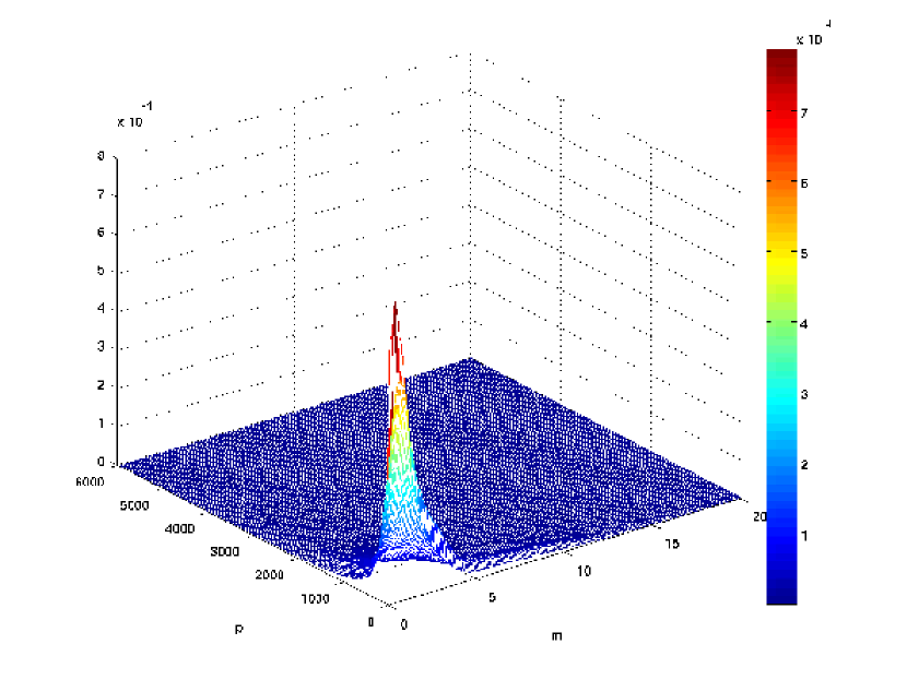
Figure 3: The three dimensional view of the coupled period-mass pdf, $f_{(P,M)}(p,m|\theta)$, of the guess-mass model.

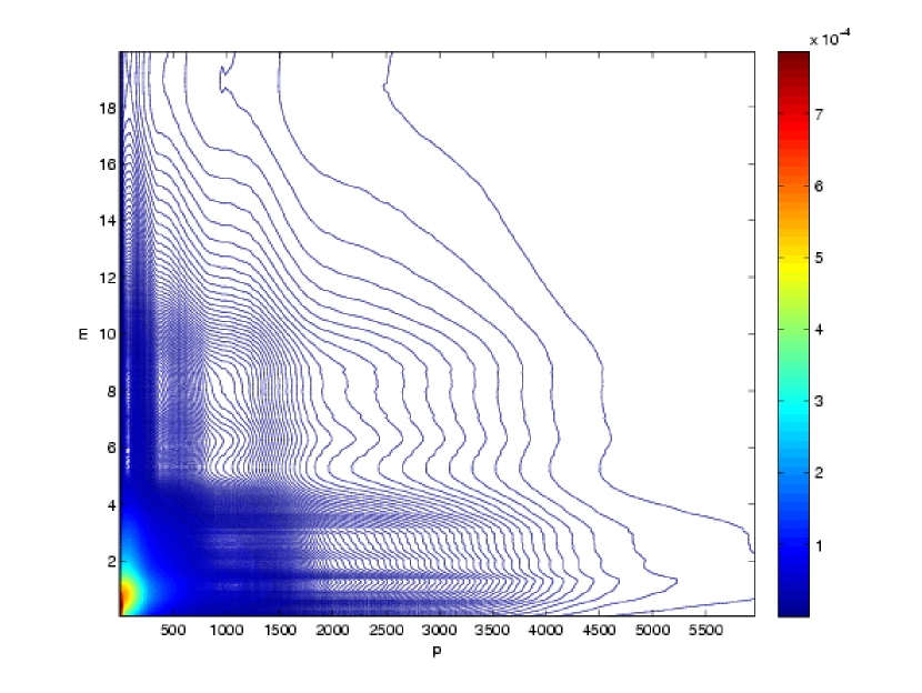
Figure 4: The color contour of the coupled period-mass pdf, $f_{(P,M)}(p,m|\theta)$, of the guess-mass model.

Figure 3 shows the three dimensional view of the coupled period-mass pdf, $f_{(P,M)}(p,m|\theta)$, of the guess-mass model. The contour of Figure 3 is presented in Figure 4. The plots of the minimum-mass model’s $f_{(P,M)}(p,m|\theta)$ are very similar to the above, so we have not shown them.

We know that when the period and mass are completely independent, $f_{(P,M)}(p,m|\theta)=f_{P}(p)f_{M}(m)$. Thus the term

$$\frac{-\theta(e^{-\theta}-1)e^{-\theta F_{P}(p)}e^{-\theta F_{M}(m)}}{\left\{e^{-\theta}-1+(e^{-\theta F_{P}(p)}-1)(e^{-\theta F_{M}(m)}-1)\right\}^{2}}$$

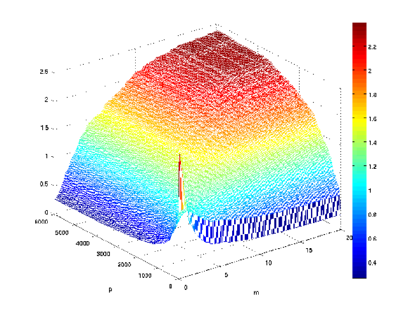
Figure 5: The three dimensional view of the Coupling Factor of the guess-mass model.

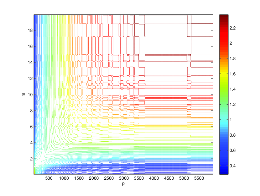
Figure 6: The color contour of the Coupling Factor of the guess-mass model.

in Eq. (4) is the one to take the period-mass coupling into account. We will hereafter call it the Coupling Factor. To make it clear how the Coupling Factor behaves, its value as a function of $p$ and $m$ of the guess-mass model is plotted in Figure 5. Figure 6 is the color contour plot. It clearly shows that the Coupling Factor becomes larger than one when both period and mass are very small or when both of them are large (area of red). It also shows that the Coupling Factor is less than one in the blue area.

5.2 The Correlation Coefficients

JYCH07 calculated the linear correlation coefficients (also called Pearson’s correlation coefficients) in both $m$-$p$ and ${\rm ln}m$-${\rm ln}p$ spaces and found a weak correlation in $m$-$p$ and a moderate correlation in ${\rm ln}m$-${\rm ln}p$ space. In order to maintain a consistent determination on the correlation coefficients, we now calculate the Spearman rank-order correlation coefficients (Press et al. 1992), which are invariant under strictly increasing nonlinear transformations (Schweizer and Sklar 2005).

For pairs of quantities $(x_{i},y_{i}),i=1,\ldots,n$, the linear correlation coefficient is given by

$$r=\frac{\sum_{i=1}^{n}(x_{i}-\bar{x})(y_{i}-\bar{y})}{\sqrt{\sum_{i=1}^{n}(x_{i}-\bar{x})^{2}\sum_{i=1}^{n}(y_{i}-\bar{y})^{2}}},$$ (9)

where $\bar{x}=\sum_{i=1}^{n}x_{i}/n$, $\bar{y}=\sum_{i=1}^{n}y_{i}/n$. The Spearman rank-order correlation coefficient is calculated by the above formula with $x_{i}$ and $y_{i}$ replaced by their ranks. Given $R(x_{i})$ the rank of $x_{i}$ and $R(y_{i})$ the rank of $y_{i}$, then the Spearman rank-order correlation coefficient can be written as

$$\rho_{S}=1-\frac{6}{n^{3}-n}\sum_{i=1}^{n}\big{[}R(x_{i})-R(y_{i})\big{]}^{2}.$$ (10)

We note that $|\rho_{S}|=1$ indicates a perfect dependence and $\rho_{S}=0$ means no dependence. When $\rho_{S}=1$ there is a direct perfect dependence and when $\rho_{S}=-1$ there is an inverse perfect dependence. Furthermore, according to Cohen (1988), $0.1<|\rho_{S}|\leq 0.3$ means the correlation is weak, $0.3<|\rho_{S}|\leq 0.5$ indicates a moderate correlation, and $0.5<|\rho_{S}|\leq 1.0$ is indicative of strong correlation.

For the minimum-mass model, the Spearman rank-order correlation coefficient is obtained as $\rho_{S}=0.3769$. Through Copula Modelling, we also find the estimate of $\rho_{G}$, which is $\hat{\rho}_{G}=0.3792$. It is obvious that the Spearman rank-order correlation coefficient $\rho_{S}=0.3769$ is very close to $\hat{\rho}_{G}$. Moreover, the 95% bootstrap C.I. with the number of bootstrap replications $B=2000$ for $\rho_{G}$ is $(0.2691,0.4811)$. For the guess-mass model, we have $\hat{\rho}_{G}=0.3899$ with a 95% bootstrap C.I. $(0.2811,0.4869)$. These results are all consistent and confirm that there is a positive period-mass correlation for exoplanets.

6 Conclusions

Using the data of exoplanets, for the first time in this field we have constructed an analytic coupled period-mass function through a nonparametric approach. Moreover, we calculate the Spearman rank-order correlation coefficient, which gives the same results for linear and logarithmic spaces, and the results in the previous section show that there is a moderate positive period-mass correlation.

In order to comprehend the implication of our results, in Figure 7(a)-(b), we plot $f_{(P,M)}(p,m|\theta)$ with $m=1,5,10,15M_{J}$ (i.e. the period functions given different masses), and also $f_{(P,M)}(p,m|\theta)$ with $p=1,50,100,150$ days (i.e. the mass functions given different periods) in logarithmic spaces. For purposes of comparing, $f_{P}(p)\times f_{M}(m)$ with $m=1,5,10,15M_{J}$ (the independent period functions) and $f_{P}(p)\times f_{M}(m)$ with $p=1,50,100,150$ days (the independent mass functions) are also plotted in Figure 7(c)-(d). Of course, the shapes of independent period functions with $m=1,5,10,15M_{J}$ are all the same, and the shapes of independent mass functions given different periods are all exactly the same as well.

We find that the period function of $m=1M_{J}$ is very similar with the independent period functions. However, the period functions of $m=5,10,15M_{J}$ are different from the independent ones, in a way that the functions are lower at the smaller $p$ end and slightly higher at the larger $p$ end. Thus, the overall period functions of massive planets (say $m=5,10,15M_{J}$) at large $p$ and small $p$ ends are closer than the one of lighter planets (say $m=1M_{J}$). Therefore, the fractions of larger and smaller $p$ (or semi-major-axis) planets are closer for those planets with mass $m=5,10,15M_{J}$.

This implies that the more massive planets have larger ranges of possible semi-major axes. This interesting statistical result will provide important clues into the theories of planetary formation.

On the other hand, the mass functions of $p=50,100,150$ days are all very similar with the independent mass functions. However, the mass function of $p=1$ day is different from the independent one in a way that the function is higher at the smaller $m$ end and lower at the larger $m$ end. Thus, the mass function of short period planets (say $p=1$ day) is steeper than the one of long period planets (say $p=50,100,150$ days). This implies that the percentage of massive planets are relatively small for the short period planets. This result reconfirms the deficit of massive close-in planets due to tidal interaction as studied in Jiang et al. (2003).

Figure 1: The cumulative distribution function (cdf) and probability density function (pdf) of planetary period and mass. (a) The period cdf. (b) The mass cdf of the minimum-mass model (solid curve) and the guess-mass model (dotted curve). (c) The histogram of planets in $p$ space and also the period pdf $\hat{f}^{h}_{P}(p)$ (solid curve). (d) The histogram of planets in $m$ space of the minimum-mass model (solid line) and the guess-mass model (dotted line), and also the mass pdf of the minimum-mass model $\hat{f}^{hm}_{M}(m)$ (solid curve) and the guess-mass model $\hat{f}^{hg}_{M}(m)$ (dotted curve).

Figure 2: The random variables $x$ and $y$ in the credibility test of Copula Modelling. (a) $\rho_{S}$= 0.042. (b) $\rho_{S}$=0.231. (c) $\rho_{S}$= 0.416 (d) $\rho_{S}$= 0.788.

Figure 7: The period and mass functions in logarithmic space. (a) The period functions of $m=1M_{J}$ (solid curve), $m=5M_{J}$ (dotted curve), $m=10M_{J}$ (short dashed curve), and $m=15M_{J}$ (long dashed curve). (b) The mass functions of $p=1$ day (solid curve), $p=50$ days (dotted curve), $p=100$ days (short dashed curve), and $p=150$ days (long dashed curve). (c) The independent period functions of $m=1M_{J}$ (solid curve), $m=5M_{J}$ (dotted curve), $m=10M_{J}$ (short dashed curve), and $m=15M_{J}$ (long dashed curve). (d) The independent mass functions of $p=1$ day (solid curve), $p=50$ days (dotted curve), $p=100$ days (short dashed curve), and $p=150$ days (long dashed curve).

References

- (1) Armitage, P. J., Livio, M., Lubow, S. H., Pringle, J. E., 2002, MNRAS, 334, 248
- (2) Boss, A. P. 2005, ApJ, 629, 535
- (3) Cohen, J, 1988, Statistical power analysis for the behavioral sciences, Lawrence Erlbaum Associates, New Jersey.
- (4) Frank, M.J. 1979, Aequationes Math, 19, 194
- (5) Frees, E.W., Valdez, E.A. 1998, North American Actuarial Journal 2, 1
- (6) Genest, C., MacKay, J. 1986, The American Statistician 4, 280.
- (7) Genets, C. 1987, Biometrika, 74, 549
- (8) Hogg, R.V., Tanis, E.A. 2006, Probability and Statistical Inference (Pearson Prentice Hall, New Jersey)
- (9) Ji, J., Kinoshita, H., Liu, L., Li, G. 2003, ApJ, 585, L139
- (10) Jiang, I.-G., Ip, W.-H. 2001, A&A, 367, 943
- (11) Jiang, I.-G., Ip, W.-H., Yeh, L.-C., 2003, ApJ, 582, 449
- (12) Jiang, I.-G., Yeh, L.-C. 2004a, MNRAS, 355, L29
- (13) Jiang, I.-G., Yeh, L.-C. 2004b, International Journal of Bifurcation and Chaos, 14, 3153
- (14) Jiang, I.-G., Yeh, L.-C. 2007, ApJ, 656, 534
- (15) Jiang, I.-G., Yeh, L.-C., Chang, Y.-C., Hung, W.-L. 2007, AJ, 134, 2061 (JYCH07)
- (16) Jiang, I.-G., Yeh, L.-C., Hung, W.-L., Yang, M.-S. 2006, MNRAS, 370, 1379
- (17) Kinoshita, H., Nakai, H. 2001, PASJ, 53, L25
- (18) Klugman, S.A., Parsa, P. 1999, Insurance: Mathematics and Economics, 24, 139
- (19) Marchi, S. 2007, ApJ, 666, 475
- (20) Mayor, M., Queloz, D. 1995, Nature, 378, 355
- (21) Press, W. H. et al. 1992, Numerical Recipes in Fortran, Cambridge University Press
- (22) Rice, W. K. M., Armitage, P. J., Hogg, D. F. 2008, MNRAS, 384, 1242
- (23) Schweizer, B., Sklar, A. 2005, Probabilistic Metric Spaces, Dover Publications, Mineola, New York
- (24) Silverman, B. W. 1986, Density Estimation for Statistics and Data Analysis, Chapman & Hall, New York
- (25) Tabachnik, S., Tremaine, S., 2002, MNRAS, 335, 151
- (26) Trivedi, P.K., Zimmer, D.M. 2005, Foundations & Trends in Econometrics, 1, 1
- (27) Tukey, W.J., 1977, Exploratory Data Analysis, Addison-Wesley, Reading, Mass.
- (28) Venter, G., Barnett, Kreps, R., Major, J. 2007, Variance 1, 103
- (29) Wolszczan, A., Frail, D. A. 1992, Nature, 355, 145
- (30) Zucker, S., Mazeh, T., 2002, ApJ, 568, L113