A Link Surgery Spectral Sequence in
Monopole Floer Homology
Jonathan M. Bloom
Abstract.
To a link , we associate a spectral sequence whose page is the reduced Khovanov homology of and which converges to a version of the monopole Floer homology of the branched double cover. The pages for depend only on the mutation equivalence class of . We define a mod 2 grading on the spectral sequence which interpolates between the -grading on Khovanov homology and the mod 2 grading on Floer homology. We also derive a new formula for link signature that is well-adapted to Khovanov homology.
More generally, we construct new bigraded invariants of a framed link in a 3-manifold as the pages of a spectral sequence modeled on the surgery exact triangle. The differentials count monopoles over families of metrics parameterized by permutohedra. We utilize a connection between the topology of link surgeries and the combinatorics of graph associahedra. This also yields simple realizations of permutohedra and associahedra, as refinements of hypercubes.
The author was supported by NSF grant DMS-0739392.
Department of Mathematics, Columbia University, New York, NY 10027, USA E-mail address:jbloom@math.columbia.edu URL:http://math.columbia.edu/~jbloom/
1. Introduction
Monopole Floer homology is a gauge-theoretic invariant defined via Morse theory on the Chern-Simons-Dirac functional. As such, the underlying chain complex is generated by Seiberg-Witten monopoles over a 3-manifold, and the differential counts monopoles over the product of the 3-manifold with . In [17], a surgery exact triangle is associated to a triple of surgeries on a knot in a 3-manifold (for a precursor in instanton Floer homology, see [4], [10]).
This paper has two main objectives. The first is to construct a link surgery spectral sequence in monopole Floer homology, generalizing the exact triangle. This is a spectral sequence which starts at the monopole Floer homology of a hypercube of surgeries on along , and converges to the monopole Floer homology of itself. The differentials count monopoles on 2-handle cobordisms equipped with families of metrics parameterized by polytopes called permutohedra. Those metrics parameterized by the boundary of the permutohedra are stretched to infinity along collections of hypersurfaces, representing surgered 3-manifolds. The monopole counts satisfy identities obtained by viewing the map associated to each polytope as a null-homotopy for the map associated to its boundary. Note that this can be seen as analogue of Ozsváth and Szabó’s link surgery spectral sequence for Heegaard Floer homology [24]. There, the differentials count pseudo-holomorphic polygons in Heegaard multi-diagrams, and they satisfy relations which encode degenerations of conformal structures on polygons. In Section 10, we develop a dictionary between these gauge-theoretic and symplectic perspectives.
Our construction introduces a number of techniques that we hope will be of more general use. In Sections 2 and 5, we couple the topology of 2-handle cobordisms arising from link surgeries to the combinatorics of polytopes called graph associahedra [5]. For the chain-level Floer maps induced by 2-handle cobordisms, these polytopes encode a mixture of commutativity and associativity up to homotopy. We hope this coupling, and its relationship to finite product lattices, will be of independent interest to algebraists and combinatorists. As one application, we obtain simple, recursive realizations of permutohedra as refinements of associahedra, which in turn refine hypercubes (see Figures 14 through 17). Curiously, these realizations are predicted by the “sliding-the-point” proof of the naturality of the action in Floer theory.
Our construction of polytopes of metrics was inspired by the pentagon of metrics in the proof of the surgery exact triangle [17]. However, to make use of these polytopes, we must deal effectively with the notorious mix of interior, boundary-stable, and boundary-unstable critical points involved in the construction of the monopole Floer complex. To this end, we systematize the construction of maps associated to cobordisms equipped with polytopes of metrics, as well as the vanishing operators which count ends of 1-dimensional moduli spaces. This includes the construction of the usual monopole Floer differentials, cobordism maps, and homotopies as special cases, as well as the operators used in the proof of the surgery exact triangle, which we reorganize in Section 6. More generally, we prove that the homotopy type of the link surgery spectral sequence is independent of analytic choices, which may be viewed as a gauge-theoretic analogue of the invariance of homotopy type in symplectic geometry [28]. In particular, the higher pages are themselves invariants of a framed link in a 3-manifold.
Khovanov homology is a powerful new invariant of classical links in the 3-sphere, arising from representation theory [14]. It is defined combinatorially and categorifies the Jones polynomial. Our second main objective is to construct a spectral sequence from reduced Khovanov homology to a version of the monopole Floer homology of the branched double cover. While here the strategy in the Heegaard Floer case may be translated fairly directly, we instead present a more global identification of the page with the reduced Khovanov complex, based on our “thriftier” construction of the reduced odd Khovanov complex [3]. The intermediate pages are link invariants as well.
Beyond these objectives, we refine the link surgery spectral sequence, as well as its specialization to Khovanov homology, in ways that were not previously known for the Heegaard Floer version, but now follow by parallel arguments. In particular, we equip the spectral sequence with a mod 2 grading which interpolates between a shift of the -grading on Khovanov homology and the mod 2 grading on monopole Floer homology, thereby refining the known rank inequality.
We also derive a new formula for the signature of a link that is well-adapted to Khovanov homology and may be of independent interest.
We have recently learned that Kronheimer and Mrowka have established a similar connection between Khovanov homology and a version of instanton Floer homology. It would be interesting to understand the relationship between our approaches.
1.1. Statement of results.
All monopole Floer homology and Khovanov homology groups are considered over the 2-element field . Our notation is consistent with the definitive reference [15]. In particular, and denote the “to” version of the complex and homology group associated to , while and denote the chain-level and homology-level homomorphisms associated to a cobordism .
In order to motivate the statement of the link surgery spectral sequence, we first recall the surgery exact triangle. Let be a closed, oriented 3-manifold, equipped with a knot with framing and meridian . Orient and as simple closed curves on the torus boundary of the complement of a neighborhood of , so that the algebraic intersection numbers of the triple satisfy
Let and denote the result of surgery on with respect to and , respectively. In [17], Kronheimer, Mrowka, Ozsváth, and Szabó prove that the mapping cone
is quasi-isomorphic to the monopole Floer complex , where is the chain map induced by the elementary 2-handle cobordism from to . The associated long exact sequence on homology is known as the surgery exact triangle. However, we can also frame the result in another way. As in [24], if we filter by the index in , then the mapping cone induces a spectral sequence with
and
which converges by the page to .
The link surgery spectral sequence generalizes this interpretation of the exact triangle to the case of an -component framed link . For each in the hypercube , let denote the result of performing -surgery on the component . For , let denote the associated cobordism, composed of 2-handles. The (iterated) mapping cone now takes the form of a hypercube complex
with differential given by the sum of components for all . We filter by vertex weight , defined as the sum of the coordinates of . The component is the usual differential on , whereas for , the component counts monopoles on over a family of metrics parametrized by the permutohedron of dimension . We define this family in Section 2 and construct in Section 4. In Section 7, we complete the proof of:
Theorem 1.1.
The filtered complex induces a spectral sequence with page given by
and differential given by
The spectral sequence converges by the page to and comes equipped with an absolute mod 2 grading which coincides on with that of . In addition, each page has an integer grading induced by vertex weight. The differential shifts by one and increases by .
The complex depends on a choice of regular metric and perturbation of the monopole equations on the full cobordism from to . For any two such choices, we produce a homotopy equivalence which induces a graded isomorphism between the associated pages.
Theorem 1.2.
For each , the -graded vector space is an invariant of the framed link .
In fact, reduced Khovanov homology over arises as such an invariant. To frame this properly, in Section 8, we introduce another version of monopole Floer homology, pronounced “H-M-hat” and denoted . By analogy with in Heegaard Floer homology, we define as the homology of the mapping cone of , where induces the usual even endomorphism on . It follows that inherits a mod 2 grading, and we prove a version of Theorem 1.1 for as well. Note that should agree with the sutured monopole Floer homology group relative to the equatorial suture, as defined in [16]. The latter is given by , where is an orientable surface of genus and is the canonical spinc-structure with . In particular, the rank of is finite over and invariant under orientation reversal.
For an oriented link , let denote the reduced Khovanov homology of . To a diagram of , we will associate a framed link in the branched double cover with reversed orientation, denoted . Applying the version of Theorem 1.1, we prove:
Theorem 1.3.
The link surgery spectral sequence for has page isomorphic to and converges by the page to .
While the construction of this spectral sequence depends on a choice of diagram for , as well as analytic data, Theorem 1.3 implies that the and pages are actually link invariants. These pages are also insensitive to Conway mutation, since this is true of Khovanov homology over as well as branched double covers. More generally, we prove:
Theorem 1.4.
For each , the -graded vector space depends only on the mutation equivalence class of .
The analytic invariance described in Theorem 1.2 is crucial here. As explained in Section 9.2, Reidemeister invariance is then an immediate consequence of Baldwin’s proof in the Heegaard Floer case [2], whereas mutation invariance follows from our proof in the Heegaard Floer case [3]. Note that both Heegaard Floer proofs, in turn, depend on Roberts’ work on invariance with respect to isotopy, handleslides, and stabilization in Heegaard multi-diagrams [26], and Baldwin’s work on invariance with respect to almost complex data [2].
Recall that Khovanov homology is graded by two integers, the homological grading and the quantum grading . We may repackage this as a rational -bigrading, where
marks the diagonals of slope two in the -plane. On the other hand, monopole Floer homology has a canonical mod 2 grading and decomposes over the set of spinc structures. Using the grading on the spectral sequence, we derive the first result relating these finer features of monopole or Heegaard Floer homology to those of Khovanov homology, leading to a refinement of the rank inequality
Let and denote the even and odd graded pieces of , respectively. Let and denote the even and odd graded pieces of with respect to the integer grading . The terms and refer to the signature and nullity of , respectively. Our convention is that the signature of the right-handed trefoil is +2 (that is, minus the signature of a Seifert matrix). Recall that .
Theorem 1.5.
The grading on the spectral sequence coincides with
on the page. Thus, the rank inequality may be refined to
Furthermore, the Euler characteristic of each page is given by .
In particular, all the differentials on the spectral sequence shift by one. We conclude:
Corollary 1.6.
If is supported on a single diagonal, then the spectral sequence collapses at the page. In particular, is supported in even grading and has rank , with one generator in each spinc structure.
In fact, is supported on the single diagonal whenever is quasi-alternating [20]. This is consistent with Theorem 1.5, since quasi-alternating links have non-zero determinant, and therefore vanishing nullity.
Finally, we present a new formula for . It follows quickly from the proof of Theorem 1.5, which in turn invokes the Gordon-Litherland signature formula (see [12]).
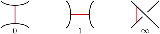
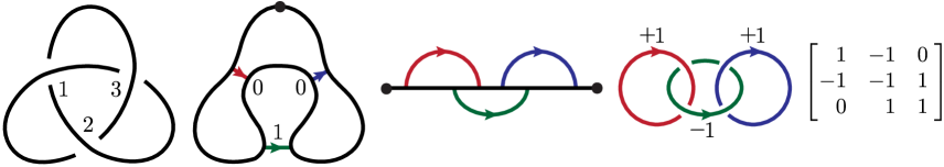
As in [3], we first assign a symmetric matrix to an oriented, connected diagram with numbered crossings as follows. Fix a vertex such that the resolution consists of one circle (such a resolution may be obtained by resolving along a spanning tree of the black graph). Now place a small arbitrarily-oriented arc across each resolved crossing, as shown at left in Figure 1. Two arcs are linked if their endpoints are interleaved around the circle. For each pair of linked arcs , set according to the convention at right in Figure 1. Here we are viewing on the sphere, so that the outside arc may be pulled to the bottom. Let and set all remaining entries to zero. Let denote the number of negative crossings in .
Proposition 1.7.
With the above conventions:
The proof and an example are given at the end of Section 9.1. Unlike the Goeritz matrix, the non-zero entries of are all . Remarkably, a deep structure theorem in graph theory due to W. H. Cunningham implies that alone determines the mutation equivalence class of , the framed isotopy type of , and therefore for all (see [3], [7], and Remark 9.3).
Figure 1. Resolution and arc-linking conventions for the signature formula.
1.2. Philosophy and future directions.
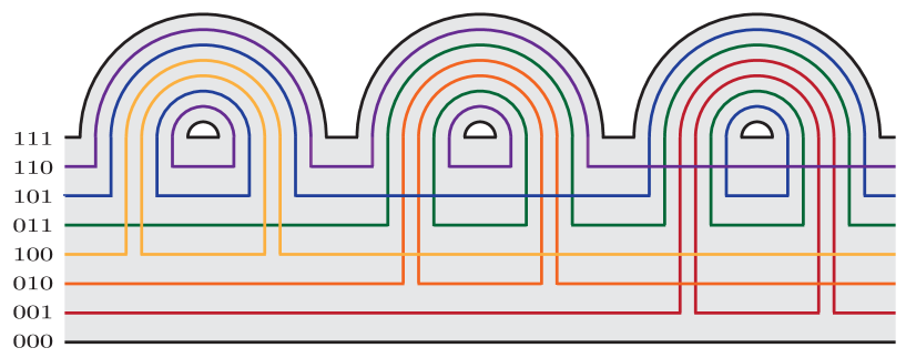
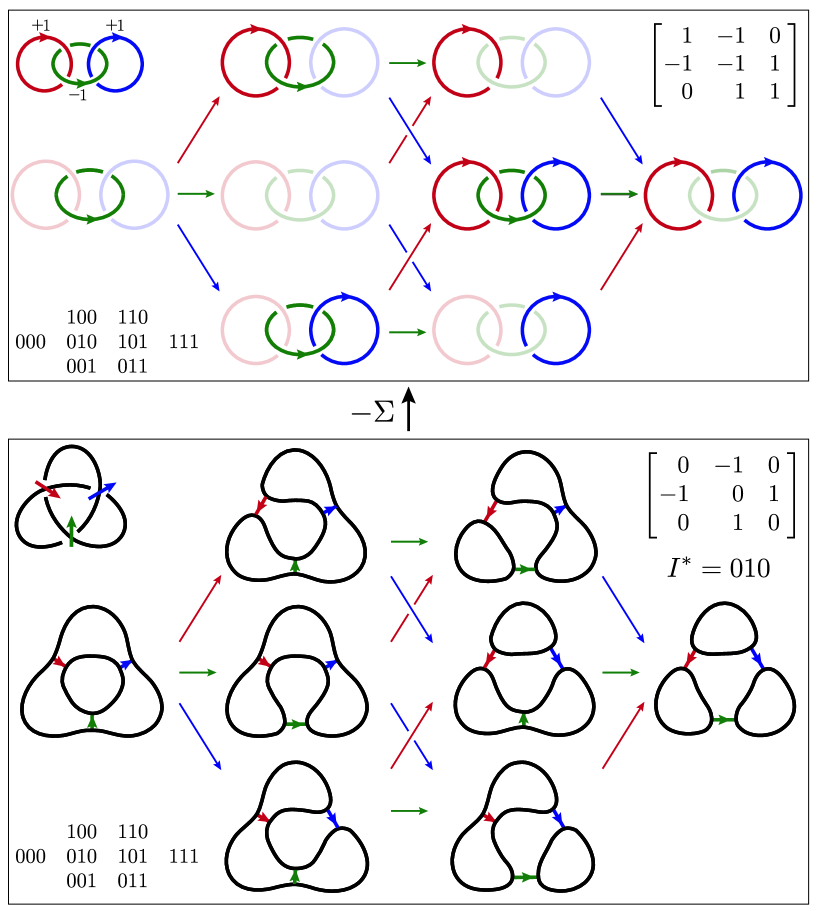
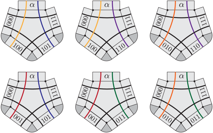
In outline, the identity of the page in Theorem 1.3 may be established as follows (our detailed proof in Section 9 is along slightly different lines). To a diagram of a link , we associate a framed link . With respect to , the link surgery hypercube of 3-manifolds and 4-dimensional 2-handle cobordisms is precisely the branched double cover of the Khovanov hypercube of 1-manifolds and 2-dimensional 1-handle cobordisms , as illustrated for the trefoil knot in Figures 19 and 20. Furthermore, the functor and the functor underlying Khovanov’s unreduced theory over fit into a commutative square of functors.
Here and represent the induced maps of -vector spaces with respect to each theory. If we replace with the reduced Khovanov functor over , then the vertical arrow at right induces an equivariant isomorphism of vector spaces. Consequently, we may identify the complex with , and hence with .
In fact, the entire commutative diagram admits a more elementary and unified description, which illuminates why the functors and are connected in the first place. Both horizontal arrows may be regarded as an instance of a TQFT described by Donaldson in [9]. The algebraic basis for his construction is as follows. To an -vector space , we associate the exterior algebra .
To a linear map , we associate a map defined as follows. Let and be the dimensions of and , respectively. By taking the exterior product of the images of the elements in any basis of , we obtain an element of , which may be regarded as a map via the series of isomorphisms
A composition law holds provided that a certain transversality condition is met.
To a manifold , Donaldson associates the exterior algebra . To a cobordism , he associates the map
obtained from the restriction . If we denote his TQFT by , then the above commutative diagram may be replaced with:
Regarding the vertical arrow at right, note that for any link with a basepoint, there is a natural map which takes a relative 1-cycle to its preimage. Dually, there is a map
which induces this arrow. Note that when has positive genus, both and vanish since the restriction map from has non-trivial kernal.
The equivalence of the two commutative diagrams may be understood as follows. The manifold admits a metric of positive scalar curvature, so it follows from Proposition 36.1.3 of [15] that is the cohomology of the Picard torus , parameterizing flat -connections on modulo gauge. The cobordism also admits a metric of positive scalar curvature, and indeed, it follows from Corollary 9.2 herein that the induced map coincides with the map on cohomology induced by the correspondence between Picard tori defined by flat connections over . As Donaldson observes, the map on cohomology induced by such a correspondence is encoded in the above TQFT. Along the bottom row, this TQFT is determined by its Frobenius algebra, which one may easily check is the same as the one underlying Khovanov homology over .
A version of the spectral sequence with coefficients is work in progress. Indeed, Donaldson’s TQFT lifts to by equipping cobordisms with homology orientations, and we then recover the monopole Floer and odd Khovanov functors in our commutative diagram. We also expect that the bigrading can be lifted and shifted to an invariant rational bigrading on the higher pages (compare with Conjecture 1.1 of [2]).
For such links, we then obtain a “higher” Khovanov homology and Jones polynomial on each page for . These are conjectured for a family of torus knots in Section 9.3. Watson has shown that Khovanov homology is not an invariant of the branched double cover [32]. One wonders whether the same is true of the bigrading on the page, and what this bigrading encodes.
Finally, we strongly suspect that the entire construction of the link surgery spectral sequence is functorial. Broadly speaking, to a framed surface in a cobordism of 3-manifolds, we would like to associate a map between the spectral sequences associated to the framed links in the 3-manifold ends. In the Khovanov specialization, the branched double cover of a classical link cobordism provides a 4-manifold with boundary, and on the page, we expect to see the associated monopole Floer map. Perhaps one could then associate a framed surface in to a combinatorial description of the link cobordism, so that Khovanov’s combinatorially-defined link cobordism maps appear on the page. This would provide a Floer-theoretic realization of the functoriality of Khovanov’s theory.
Acknowledgements. It is my pleasure to thank: my advisor Peter Ozsváth, for recommending this engaging topic and providing invaluable guidance throughout. Tim Perutz, for first suggesting the relevance of Donaldson’s TQFT, and for sharing his expertise in all applicable fields. Adam Knapp and John Baldwin, for their endless enthusiasm and many insightful discussions. Satyan Devadoss, for a wonderful visit and for [8]. Dave Bayer, for his interest in my work and expert programming assistance. I am also indebted to the following people for their wisdom and support: Eli Grigsby, Robert Lipshitz, Max Lipyanskiy, Maria Lissitsyna, James Stasheff, Dylan Thurston, and Rumen Zarev.
2. Hypercubes and permutohedra
This section involves no Floer homology whatsoever, but rather surgery theory and Kirby calculus as described in Part 2 of [11]. In particular, with respect to a 2-handle , the terms core, cocore, and attaching region will refer to the subsets , , and , respectively.
Let be a closed, oriented 3-manifold, equipped with an -component, framed link , and let denote the result of (integral) surgery on . There is a standard oriented cobordism , built by thickening to and attaching 2-handles to by identifying the attaching region of with a tubular neighborhood in accordance with the framing. The diffeomorphism type of is insensitive to whether the handles are attached simultaneously as above, or instead in a succession of batches which express as a composite cobordism. Our goal in this section is to construct a family of metrics on , parameterized by the permutohedron , which smoothly interpolates between all ways of expressing as a composite cobordism.
In order to keep track of the ways to build up one handle at a time, we introduce the hypercube poset , with if and only if for all . is called an immediate successor of if there is a such that , , and for all . We define a path of length from to to be a sequence of immediate successors . The weight of a vertex is given by . We use and as shorthand for the initial and terminal vertices of , which we call external. The other vertices will be called internal. A totally ordered subset of a poset is called a chain. A chain is maximal if it is not properly contained in any other chain. In , the maximal chains are precisely the paths from to , with each such path determined by its internal vertices.
To each vertex , we associate the 3-manifold obtained by surgery on the framed sublink
in . Note that the remaining components of constitute a framed link in .
Remark 2.1.
The 3-manifold denoted in the introduction and in [24] is obtained from by shifting forward one frame in the surgery exact triangle for each component of . We will use throughout and address this discrepancy in Remark 4.12.
We regard as a poset isomorphic to , with and external and the rest internal. To a pair of vertices with , we associate the 2-handle cobordism
from to . In particular, if is an immediate successor of , then is an elementary cobordism, given by a single 2-handle addition. More generally, will be the composition of elementary cobordisms.
In order to quantify how far two vertices are from being ordered, we define a symmetric function on pairs of vertices by
Note that if and only if and are ordered. In this case, and are disjoint:
Lemma 2.2.
The full set of internal hypersurfaces can be simultaneously embedded in the interior of the cobordism so that the following conditions hold:
(i)
the hypersurfaces in any subset are pairwise disjoint if and only if they form a chain. In this case, cutting on breaks into the disjoint union
(ii)
distinct hypersurfaces and intersect in exactly disjoint tori.
Remark 2.3.
The reader who is convinced by Figure 2 may safely skip the proof.
Figure 2. Half-dimensional diagram of the cobordism for the hypercube .
Proof.
We list all of the vertices as , first in order of increasing weight and then numerically within each weight class. We express the full cobordism as
and embed and as the boundary. We then embed the interior hypersurfaces as follows. For , define a slimmer 2-handle as the image of in , where is the disk of radius . Let be the region to which is attached, considered as a subset of . Then we may regard
as a longer 2-handle which tunnels through in order to attach to along . In this way, we embed in as
and as a component of the boundary.
Now consider two vertices and and assume without loss of generality that . By construction, is confined to the union of the thickened attaching regions in with . If as well, then is contained in the interior of . On the other hand, if then and intersect in the solid torus . It follows that and intersect in one torus for each such that . With , the number of such is exactly , verifying (ii). The first part of (i) immediately follows, since a subset of forms a chain if and only if vanishes on every pair of vertices in the subset. In this case, decomposes as claimed by construction.
∎
We are now ready to build a special family of metrics on the cobordism , starting from an initial Riemannian metric which is cylindrical near every . Fix a path from to . By Lemma 2.2, corresponds to a maximal subset of disjoint internal hypersurfaces in . So for each point , we may insert necks to express as the Riemannian cobordism given by
(1)
We then extend this family to the cube by degenerating the metric on when . As in the proof of the composition law, when grows, the -neck stretches, and when , it breaks. In particular, has the metric , while is the disjoint union of elementary cobordisms which compose to give with metric .
In this way, we obtain families of metrics on , each parameterized by a cube . The facets of each cube fall evenly into two types. A facet is interior if it is specified by fixing a coordinate at 0, and exterior if it is specified by fixing a coordinate at . Note that each “almost maximal” chain can be completed to a maximal chain in exactly two ways. It follows that each internal facet has a twin on another cube, in the sense that the twins parameterize identical families of metrics on . By gluing the cubes together along twin facets, we can build a single family of metrics which interpolates between the various ways of expressing as a composite cobordism. In fact, this construction realizes the cubical subdivision of the following ubiquitous convex polytope.
The permutohedron of order arises as the convex hull of all points in whose coordinates are a permutation of . These points lie in general position in the hyperplane , so has dimension . The first four permutohedra are the point, interval, hexagon, and truncated octohedron (see Figure 4). The 1-skeleton of is the Cayley graph of the standard presentation of the symmetric group on letters:
More generally, the -dimensional faces of correspond to partitions of the set into an ordered -tuple of subsets . Inclusion of faces corresponds to merging of neighboring .
The connection between the permutohedron and the hypercube rests on a simple observation: the face poset of is dual to the poset of chains of internal vertices in the hypercube . Namely, to each face , we assign the chain , where has coordinate 1 if and only if . For example, in the case of the edges of the hexagon , the correspondence is given by:
In particular, each path from to corresponds to a vertex of .
Now in the cubical subdivision of , we may identify the cube containing with the cube of metrics so that twin interior facets are identified (see Figures 3 and 4). In this way, the interior of parameterizes a family of non-degenerate metrics on , while the boundary parameterizes a family of degenerate metrics. The parameterization can be made smooth on the interior by a slight adjustment of the rate of stretching. We summarize these observations in the following proposition.
Proposition 2.4.
The face poset of the permutohedron is dual to the poset of chains of internal hypersurfaces in . In particular, the facets of correspond to the ways of breaking into a composite cobordism along a single interior hypersurface. The interior of smoothly parameterizes a family of non-degenerate metrics on , which extends naturally to the boundary in such a way that the interior of each face parameterizes those metrics which are degenerate on precisely the corresponding chain.
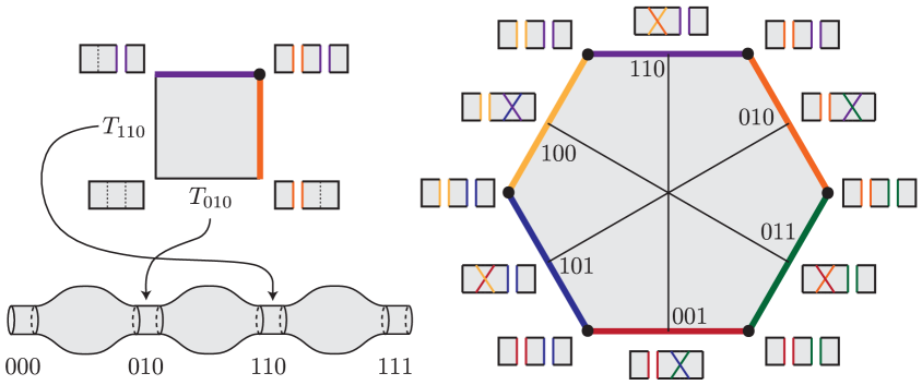
Figure 3. At left, we consider the path given by in . The corresponding square with coordinates parameterizes a family of metrics on the cobordism which stretches at and . We have one square for each non-intersecting pair of hypersurfaces in Figure 2. These six squares fit together to form the hexagon at right. The small figures at the vertices and edges illustrate the metric degenerations on , read as composite cobordisms from left to right.Figure 4. The cubical subdivision of the permutohedron consists of 24 cubes, corresponding to the paths from to in . Above, the cube corresponding to the path is shown with its exterior faces in translucent color. Each cube shares one vertex with and has one vertex at the center.
Remark 2.5.
We describe an alternative view of the above construction which is not essential, but will be helpful in Section 5 when we consider more general lattices than the hypercube. Consider the directed graph associated to , with an edge from to whenever is an immediate successor of . Let be the transitive closure of . The nodes of correspond to internal hypersurfaces, and by Lemma 2.2, two nodes are joined by an edge if and only if the corresponding internal hypersurfaces are disjoint. In fact, is the 1-sleleton of a simplical complex , whose face poset is isomorphic to the poset of non-empty cliques in under inclusion. Then is dual to the boundary of .
3. The composition law
To set notation and motivate the constructions in Section 4, we recall the formal properties of monopole Floer theory and the proof of the composition law, following [15] (see also [17] for an efficient survey). We will always work over the 2-element field . Let COB be the category whose objects are compact, connected, oriented 3-manifolds and whose morphisms are isomorphism classes of connected cobordisms. Then the monopole Floer homology groups define covariant functors from the oriented cobordism category COB to the category MOD† of modules for the ring :
The module structure may be extended over the exterior algebra . These modules have a canonical mod 2 grading, and fit into a long exact sequence
which is natural with respect to the maps induced by cobordisms. The map
induced by a cobordism satisfies the composition law
(2)
whenever is the composition of cobordisms and . The composition law follows from a “stretching the neck” argument, as do many of the results in this paper, so we now take a moment to review the proof (see Proposition 4.16 of [17] for details over , and Proposition 26.1.2 of [15] for details over ).
We refer the reader to [15] for the full construction of the monopole Floer groups. We first summarize the construction of the chain map which induces . Here the monopole Floer complex is the -vector space over the basis indexed by (irreducible or boundary stable) monopoles . Given a cobordism equipped with a metric and perturbation which are cylindrical near the boundary, we denote by the Riemannian manifold built by attaching the infinite cylinders to each end of . For monopoles and , and a relative homotopy class from to in the configuration space , we consider the moduli space of trajectories (mod gauge) on asymptotic to and and in class . The map is defined to count isolated trajectories in such moduli spaces. In particular, when is irreducible, the coefficient of in is the number of trajectories in , summed over all such that is 0-dimensional. When is 1-dimensional, it has a compactification formed by considering broken trajectories as well. The composite maps and then count the (even) number of boundary points, so
and we conclude that is a chain map.
More generally, suppose we have a family of metrics on , smoothly parameterized by a closed manifold . The map is defined to count isolated trajectories in the union
(3)
of fiber products
(4)
where denotes with the metric over . The compact fiber product is defined similarly. By counting boundary points of , we again conclude
On the other hand, if is a compact manifold with boundary , then is no longer a chain map, because the boundary of now includes the fibers over . Including these contributions, we have
(5)
Thus, is null-homotopic and provides the chain homotopy. That is independent of the choice of metric and perturbation follows by letting be the interval parameterizing a path between two such choices.
Now let be a composite cobordism
and fix a metric on which is cylindrical near each . For each , we construct a new Riemannian cobordism by cutting along and splicing in the cylinder with the cylindrical metric.
We also define as the disjoint union . In this way, parameterizes a family of metrics on , where the metric degenerates on at infinity. In other words, as increases, the cylindrical neck stretches, and when , it breaks.
We again define to count isolated trajectories in the fiber products of (3), where now
(6)
and the inner union is taken over homotopy classes and which concatenate to give . The compact fiber product is defined similarly. By counting boundary points, we conclude
(7)
Here and count trajectories in the fibers over and , respectively. Viewing as a chain homotopy, the composition law now follows. Note that, while formally similar, (5) does not imply (7) because the latter involves a degenerate metric. The key technical machinery behind this generalization consists of compactness and gluing theorems for moduli spaces on cobordisms with cylindrical ends, as developed in [15] and [17]. Our workhorse version is Lemma 4.3 in the following section.
4. The link surgery spectral sequence: construction
Let be the cobordism associated to surgery on a framed link . In Section 2, we constructed a family of metrics on , parameterized by a permutohedron and degenerate on the boundary . We now use such families to define maps between summands in a hypercube complex associated to the framed link. That these maps define a differential will follow from a generalization of (5) similar in spirit to (7). The link surgery spectral sequence is then induced by the filtration on the hypercube complex given by vertex weight.
Fix a regular metric and perturbation on the cobordism which are cylindrical near every hypersurface . Let be the direct sum of the monopole Floer complexes of the hypersurfaces, considered as a vector space over :
We will define a differential as the sum of maps over all , with the differential on the monopole Floer complex . We now construct the maps when .
Fix vertices and let . Regarding as the cobordism arising by surgery on a k-component, framed link in , with initial metric induced by , we apply Proposition 2.4 to obtain a family of metrics on parameterized by the permutohedron of dimension . Consider a pair of critical points and , and a relative homotopy class from to in the configuration space . As in (6), we must extend the definition of to the degenerate metrics over the boundary of . If is in the interior of the face , then an element of is a -tuple
where
and the homotopy classes of these elements compose to give . Here, the metric on is the restriction of the metric on . We then define as the fiber product
In order to count the points in this moduli space, we define two elements of by
(10)
(13)
Remark 4.1.
When , we replace in (10) by the moduli space of unparameterized trajectories on the cylinder (see the definition below). We similarly replace in (13) by .
Recall that , , and are vector spaces over , with bases indexed by the monopoles in , , and , respectively. We use the above counts to construct eight linear maps , , , , , , , , where for example,
(16)
Note that the above two maps are distinct. We then define by the matrix
(19)
with respect to the decomposition . The motivation behind this definition is explained in Appendix I, and we write our this map in full for in Appendix II. Finally, as promised, we let be the sum
We now turn to proving that is a differential. As in the proof of the composition law, the argument proceeds by constructing an appropriate compactification of and counting boundary points. We first consider the compactification of the space of unparameterized trajectories on , repeating nearly verbatim the definitions given in Section 16.1 of [15]. A trajectory belonging to is non-trivial if it is not invariant under the action of by translation on the cylinder . An unparameterized trajectory is an equivalence class of non-trivial trajectories in . We write for the space of unparameterized trajectories. An unparameterized broken trajectory joining to consists of the following data:
an integer , the number of components;
an -tuple of critical points with and , the restpoints;
for each with , an unparameterized trajectory in , the th component of the broken trajectory.
The homotopy class of the broken trajectory is the class of the path obtained by concatenating representatives of the classes , or the constant path at if . We write for the space of unparameterized broken trajectories in the homotopy class , and denote a typical element by . This space is compact for the appropriate topology (see [15], Section 24.6). Note that if is the class of the constant path at , then is empty, while is a single point, a broken trajectory with no components.
We are now ready to define the compactification . If is in the interior of the face , then an element of is a -tuple
where
and is in the homotopy class . The fiber product
is compact for the appropriate topology (see [15], Section 26.1). We also write for the restriction of to the fibers over the boundary . We can similarly define a compactification of by only considering reducible trajectories. Fix a regular choice of metric and perturbation.
Remark 4.2.
The intuition behind the following classification of ends comes from the model case of Morse homology for manifolds with boundary. We encourage the interested reader to see Appendix I at this time.
Lemma 4.3.
If is -dimensional, then it is compact. If is -dimensional and contains irreducibles, then is a compact, -dimensional space stratified by manifolds. The -dimensional stratum is the irreducible part of , while the -dimensional stratum (the boundary) has an even number of points and consists of:
(A)
trajectories with two or three components. In the case of three components, the middle one is boundary-obstructed.
(B)
the reducibles locus in the case that the moduli space contains reducibles as well (which requires to be boundary-unstable and to be boundary-stable).
If is -dimensional, then it is compact. If is -dimensional, then is a compact, -dimensional -manifold with boundary.
The boundary has an even number of points and consists of:
(C)
trajectories with exactly two components.
Proof.
This is essentially Lemma 4.15 of [17], which in turn is a generalization of the gluing theorems in [15] leading up to the proof of the composition law (see Corollary 21.3.2, Theorem 24.7.2, and Propositions 24.6.10, 25.1.1, and 26.1.6).
∎
Remark 4.4.
When , Lemma 4.3 holds with , , , and replaced by , , , and , respectively.
We obtain a number of identities from the fact that these moduli spaces have an even number of boundary points. We now bundle these identities into a single operator , constructed by analogy with . Fix a pair of critical points and , and a relative homotopy class from to in the configuration space . We define two elements of by
Remark 4.5.
When , we again replace and by and , respectively.
Remark 4.6.
Trajectories of type (A) necessarily have at least one irreducible component. It follows that if is 1-dimensional and does not contain irreducibles, then it can only have boundary points in strata of type (C). So the condition “if dim ” is equivalent to the usual condition “if dim and contains irreducibles.” A similar remark holds for the definition of .
By Lemma 4.3 and the above remark, counts the boundary points of when it is 1-dimensional and contains irreducibles, and is zero otherwise. Similarly, counts the boundary points of when it is 1-dimensional, and is zero otherwise. Since the number of boundary points is even, we conclude:
(20)
We proceed by analogy with , using to define linear maps , , , and , and to define linear maps and (we will not need or ). Again, these maps all vanish identically by (20). Each of these maps can be expressed as a sum of terms which are themselves compositions of the component maps of . Finally, we define the map by the matrix
(23)
It follows that vanishes identically as well. Note that the motivation behind the definition of is explained in Appendix I, with the cases written out in full in Appendix II.
Lemma 4.7.
is equal to the component of from to :
Proof.
We must show that corresponding matrix entries are equal, that is
After expanding out the and distributing, all terms on the right appear exactly once on the left by Lemma 4.3 (the terms with four components appear only once since is not a term of ). All other terms on the left are of the form , , or . In the first case, is a term of both and . Similarly, occurs in and , and occurs in and . Therefore, each of the extra terms occurs twice and we have equality over .
∎
Remark 4.8.
An internal restpoint of is called a break. A break is good if the corresponding monopole is irreducible or boundary-stable. A trajectory occurs in the extended boundary of a 1-dimensional stratum if can be obtained by appending (possibly zero) additional components to either end of a boundary point of a 1-dimensinal moduli space or . In these terms, we have shown that among the trajectories counted by , those with no good break each occur in the extended boundary of exactly two 1-dimensional strata. The remaining trajectories each have one good break and occur in the extended boundary of exactly one 1-dimensional stratum. In particular, counts those isolated trajectories which break well on . This remark may also be understood from the perspective of path algebras, as explained in Appendix I.
Remark 4.9.
A break of is central if it is not internal to or . Note that has a central break if and only if it lies over a boundary fiber. So we can express as the sum of similarly defined maps and , which count boundary points with and without a central break, respectively. It follows from Remark 4.8 that
may be thought of (imprecisely) as an operator associated to the interior of , while is (precisely) the operator associated to the boundary (in the case in Figure 3, is the sum of six composite operators, one for each edge of the hexagon). We can then express as
which has the form
This is the sense in which Lemma 4.7 should be viewed as a generalization of (5). As in that case, is null-homotopic and provides the chain homotopy. In Appendix II, we have written out the operator in full in the case .
We now conclude:
Proposition 4.10.
is a filtered chain complex, where is the filtration induced by weight, namely
Proof.
The equation holds by Lemma 4.7 and the fact that the operators all vanish identically. The differential respects the filtration, as implies .
∎
In order to describe , we recall some topology. Let be a closed, oriented 3-manifold, equipped with an oriented, framed knot , and let be the result of surgery on (this surgery is insensitive to the orientation of ). comes equipped with a canonical oriented, framed knot , obtained as the boundary of the cocore of the 2-handle in the associated elementary cobordism, and given the -1 framing with respect to the cocore (see Section 42.1 of [15] for details). So we may iterate this surgery process, yielding a sequence of pairs . It is well-known that this sequence is 3-periodic, in the sense that for each , there is an orientation-preserving diffeomorphism
which carries the oriented, framed knot to . Applying this construction to each component of the link , we may extend our collection of surgered 3-manifolds from the hypercube to the lattice . We may now state the 2-handle version of the link surgery spectral sequence, which computes in stages.
Theorem 4.11.
Let be a closed, oriented 3-manifold, equipped with an -component framed link . Then the filtered complex induces a spectral sequence with -term given by
and differential given by
The link surgery spectral sequence collapses by stage to . Each page has an integer grading induced by vertex weight, which the differential increases by .
Remark 4.12.
The above statement uses different notation than that given in Theorem 1.1 in the introduction and in Theorem 4.1 of [24], emphasizing 2-handle addition over surgery. To reconcile the two forms, we describe the 3-periodicity above in the case of a knot from the surgery perspective (see Section 42.1 of [15]). The complements are all diffeomorphic, so we may view each of the surgered manifolds as obtained by gluing a solid torus to the fixed complement . If we denote the meridian and framing of by and , respectively, thought of as curves on the torus , then we have the relations
which correspond to the matrix
of order 3. Since the framing is insensitive to the orientation of the curve, we can regard , , and as having the framings , , and , respectively. Therefore, is shifted one step from , i.e. , , and . So Theorem 1.1 is simply Theorem 4.11 applied to . In the case of a link, the same shift in the 3-periodic sequence occurs in each component.
All but the final claim of Theorem 4.11 follow immediately from the usual construction of the spectral sequence associated to a filtered complex, in this case . The grading is well-defined since each differential is homogenous with respect to vertex weight. We complete the proof in two stages. First, in Section 5, we will define a complex , modeled on the lattice , in which sits as a subcomplex. Then, in Section 6, we use the surgery exact triangle to conclude that is null-homotopic. The identity of the term quickly follows.
5. Product lattices and graph associahedra
Consider the lattice , with the product order induced by the convention . An digit contributes two to the weight. We will sometimes also use to denote the final vertex , with the meaning clear from context. Consider the full cobordism from to , the result of attaching two rounds of 2-handles:
Here is attached to the component of , and is attached to , where denotes the boundary of the co-core of with -1 framing. A valid order of attachment corresponds to a maximal chain in , or equivalently to a path in from to , of which there are . For each vertex , we have the hypersurface , diffeomorphic to a boundary component of
An digit corresponds to attaching a stack of two 2-handles to a component of .
As in Section 2, we will construct a polytope of metrics on the cobordism for all pairs of vertices . The simplest new case occurs when , , and . Since , the polytope should be a closed interval with degenerate metrics over the two boundary points. However, we now have only one interior hypersurface, , on which to degenerate the metric. The solution, as in [17], is to construct an auxiliary hypersurface as follows. Let be the 2-sphere formed by gluing the cocore of to the core of along their common boundary . Due to the -1-framing on , is a -bundle of Euler class -1, with embedded as the zero-section. It follows that
and we define the hypersurface to be the bounding 3-sphere . is then identified with the interval , with the metric degenerating on at and at .
For the lattice , we will embed auxiliary 3-spheres in addition to the internal hypersurfaces. We must then construct a family of metrics which interpolates between the ways to decompose along pairwise-disjoint hypersurfaces. As a first step, we generalize Lemma 2.2. The following proposition is motivated by a half-dimensional diagram in the spirit of Figures 2 and Figure 9.
Proposition 5.1.
The full set of internal hypersurfaces and spheres can be simultaneously embedded in the interior of so that the following conditions hold:
(i)
The internal hypersurfaces in any subset are pairwise disjoint as submanifolds of if and only if they form a chain. In this case, cutting along breaks into the disjoint union
(ii)
Distinct and intersect in exactly disjoint tori.
(iii)
and intersect if and only if , where . In this case, they intersect in a torus.
(iv)
The are pairwise disjoint.
Proof.
List the vertices as , first in order of increasing weight and then numerically within each weight class. We express the full cobordism as
and embed and as the boundary. As in the proof of Lemma 2.2, for each , we have slimmer 2-handles and as the images of in and , respectively, where is the disk of radius . Again, we think of
as a longer 2-handle which tunnels through in order to attach to along . Let be the boundary of the cocore of , so that is the region of to which attaches. Let be the annulus given in polar coordinates by , thought of as sitting in the cocore of . The boundary of consists of and a radial contraction of into the interior of , denoted . So we may regard
as a longer 2-handle which tunnels through in order to attach to along . In this way, we embed in as
and as a component of its boundary. Here . Next, let the 2-sphere be the result of gluing the cocore of and the core of along their common boundary , and let be the result of gluing together the corresponding trivial -bundles of radius . Then is a -bundle of Euler class -1, and we embed the 3-sphere as its boundary.
Conditions (i) and (ii) now follow from a straightforward generalization of the proof of Lemma 2.2. For (iii), note that if , then the intersection of and is the boundary of the restriction of the -bundle to . Finally, the are pairwise disjoint because they live in different pairs of handles.
∎
For fixed , the interval takes the form for some pair of non-negative integers with . In order to define the maps in general, we need to construct a polytope of dimension for each pair . We define abstractly to have a face of co-dimension for every subset of mutually disjoint hypersurfaces in the interior of , with inclusion of faces dual to inclusion of subsets. Our definition is justified by Theorem 5.3, which realizes concretely as a convex polytope.
In order to motivate this theorem, we first construct those of dimension three or less by hand. The polytopes , , , and are the first few permutohedra of Proposition 2.4, namely a point, an interval, a hexagon, and a truncated octahedron (recall Figure 4). We saw that is an interval, and it is easy to see that is the associahedron , otherwise known as the pentagon. is more interesting. In Figure 5, we use a trick to establish that it is , also known as Stasheff’s polytope [30]. For a fun and informal introduction to associahedra, see [6]. Note that has dimension , while has dimension .
Figure 5. Consider the full cobordism corresponding to the lattice at left. The seven interior hypersurfaces and two auxiliary 3-spheres are embedded in in such a way that the diagram at center accurately depicts which pairs intersect (although the triple intersection point is an artifact). The nine internal arcs in the diagram are arranged so that by stretching normal to disjoint subsets, we obtain a parameterization of the space of conformal structures on the hexagon, which is known to compactify to the associahedron at right. This connection between associahedra and conformal structures on polygons leads to a dictionary between the techniques in this paper and their counterparts in Heegaard Floer homology, as explained in Section 10.
At this stage, it may be tempting to conjecture that all the are permutohedra or associahedra. We check this against the only remaining 3-dimensional case, namely . To build this polyhedron, it is useful to return to the viewpoint of Remark 2.5. Let be the oriented graph corresponding to the lattice . Let be the unoriented graph obtained as the transitive closure of with its initial and final nodes removed. We now add additional nodes (representing the ) to and connect each to the others and to those with . By Proposition 5.1, the nodes of the resulting graph are in bijection with the full set of hypersurfaces, with two nodes connected by an edge if and only if the corresponding hypersurfaces are disjoint. The graph is the 1-skeleton of a simplical complex whose face poset is isomorphic to the poset of non-empty cliques in under inclusion. That is, the -dimensional faces of are in bijection with the -cliques of (the fact that this poset defines a simplicial complex will follow from Theorem 5.3). The simple polytope dual to is then, by definition, the boundary of . In Figure 6, we illustrate this process for , concluding that it is indeed something new.
Figure 6. We construct the boundary of the polyhedron as the dual of the simplicial complex . First, at left, we remove the initial and final nodes from the lattice . We then flatten the shaded region and take the transitive closure to obtain , represented by the shaded rectangle and compact dotted line segments at center. Next we add the vertex at infinity (not shown) and connect it by dotted lines to the six nodes for which . At this stage, we have constructed , the 1-skeleton of . The faces of are the 3-cliques (triangles). Drawing the dual with thin red lines, we obtain the boundary of . At right, we have redrawn . The face corresponds to the large hexagonal base under the colorful tortoise shell. The 12 vertices away from correspond to the 12 paths through the lattice.
The right hand side of Figure 6 illustrates as a convex polytope in . However, our dual-graph perspective does not provide such an explicit realization of in higher dimensions. While searching for an alternative construction of , the author discovered beautiful illustrations of similar polyhedra in [5] and [8]. Given a connected graph with vertices, Carr and Devadoss construct a convex polytope of dimension , the graph-associahedron of , using the following notions.
A tube of is a proper, non-empty set of nodes of whose induced graph is a connected subgraph of . There are three ways in which tubes and can interact:
(1)
Tubes are nested if or ;
(2)
Tubes intersect if and and ;
(3)
Tubes are adjacent if and is a tube in .
Tubes are compatible if they do not intersect and they are not adjacent. A tubing of is a set of tubes of such that every pair of tubes in is compatible.
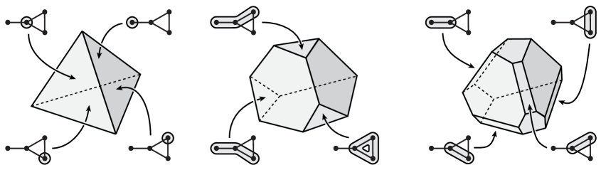
We now define the graph-associahedron of a connected graph with nodes. Labelling each facet of the simplex by a node of , we have a bijection between the faces of and the proper subsets of nodes of . By definition, is sculpted from by truncating those faces which correspond to a connected, induced subgraph of (see Figure 7). We therefore have a bijection
(24)
More generally, Carr and Devadoss prove that is a simple, convex polytope whose face poset is isomorphic to the set of valid tubings of , ordered such that if is obtained from by adding tubes. Moreover, in [8], Devadoss derives a simple, recursive formula for a set of points with integral coordinates in , whose convex hull realizes .
Remark 5.2.
Carr and Devadoss trace their construction back to the Deligne-Knudsen-Mumford compactification of the real moduli space of curves. In this context, the sculpting of is thought of as a sequence of real blow-ups. When is a Coxeter graph, tiles the compactification of the hyperplane arrangement associated to the corresponding Coxeter system. The -node clique, path, and cycle yield the -dimensional permutohedron, associahedron, and cyclohedron, respectively.
Figure 7. We have modified Figure 6 in [8] to illustrate the sculpting of for the graph given by the 3-clique with one leaf. Each node of slices out a half-space in , leaving the 3-simplex at left. Next, we shave down those vertices of which correspond to the connected, induced subgraphs of size three. Finally, at right, we shave down those edges of which correspond to the edges of . This figure also illustrates the bijection (24).
Comparing Figures 6 and 7, we see that is precisely the graph-associahedron of the 3-clique with one leaf (recall that the -clique is the complete graph on vertices). In fact, all of the polytopes are graph-associahedra:
Theorem 5.3.
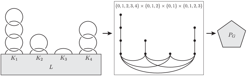
The polytope associated to the lattice is the graph-associahedron of the -clique with leaves. More generally, the polytope naturally associated to the lattice , with all , is the graph-associahedron of the -clique with paths of length attached.
Proof.
An example is given in Figure 8. We first consider the lattice . In addition to the internal hypersurfaces , we have auxialliary hypersurfaces . Let be the complete graph on nodes with a leaf attached to for each . The bijection (24) is given by
and extends to an isomorphism of posets.
Next, consider the lattice . The cobordism is then built by attaching a single stack of handles to (the case is shown in Figure 9, though with different notation). In addition to the internal hypersurfaces , we include an auxiliary hypersurface between each pair of handles with , embedded as the boundary of a tubular neighborhood of the union of the intervening 2-spheres . In fact, if (mod 3), then is diffeomorphic to . Otherwise, is diffeomorphic to . By a straightforward variation on the theme of Lemma 2.2 and Proposition 5.1, these hypersurfaces can all be embedded in in such a way that
(i)
the are all disjoint;
(ii)
and intersect if and only if . In this case, they intersect in a torus.
(iii)
and intersect if and only if the intervals and overlap but are not nested. In this case, they intersect in a torus.
Now let the graph be the path with nodes . The bijection (24) is given by
and extends to an isomorphism of posets. As remarked above, is then the -dimensional associahedron . The result for a lattice consisting of an arbitrary product of chains follows from a straightforward, subscript-heavy amalgamation of the arguments in the above two cases.
∎
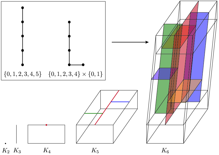
Figure 8. The figure at left represents a Kirby diagram arising from the 3-periodic surgery sequence applied to each component of a framed link with four components. The corresponding lattice is the product of four chains, while the graph is obtained by appending paths to the complete graph on four vertices. The pentagon at right represents the corresponding 9-dimensional graph associahedron. The above assignment of a polytope to a finite product lattice generalizes the assignment of the permutohedron to the hypercube described in Section 2.
Now consider the lattice with the corresponding graph given by Theorem 5.3. Using a formula in [8], we can realize concretely as the convex hull of vertices in general position in , where . Now has one vertex for every maximal collection of disjoint hypersurfaces in the cobordism with initial metric . As in Section 2, we associate to the vertex a cube of metrics which stretches on the hypersurfaces in . We can then use to parameterize a family of metrics on by identifying each with the cube containing the vertex in the cubical subdivision of . In particular, consists of cubes.
Remark 5.4.
Using these polytopes of metrics, we can define maps associated to any lattice formed as a product of chains of arbitrary length, where has length . However, we will see that this gives rise to a differential if and only if all the chains have length one or two. When there is a chain of length three or more, additional terms arise from breaks on auxiliary hypersurfaces. We will see this phenomenon explicitly for a single chain of length three in the proof of the surgery exact triangle (see Theorem 6.2).
Having constructed polytopes of metrics for all intervals in the lattice , we proceed to define the complex . Fix a metric on the cobordism which is cylindrical near every hypersurface and auxiliary hypersurface , where each has been equipped with the round metric.
We let
and define the maps by exactly the same construction and matrix (19) as before, with their sum.
We now prove that is a differential by an argument which parallels that in Section 4. We first expand our definition of to intervals of the form . Let denote the copy of cut out by . For each , let be the spheres completely contained in . We denote the corresponding cobordism with boundary components by
If is in the interior of the face , then an element of is a -tuple
(25)
where
and is in the homotopy class (and similarly when is in the interior of a face which includes a subset of the other than the first ).
The fiber product
is compact. We then define by exactly the same construction and matrix (23) as before.
We will also need the following lemma, consolidated from [17] (see Lemma 5.3 there and the preceding discussion). The essential point is that there is a diffeomorphism of which restricts to the identity on the boundary and induces a fixed-point-free involution on the set of spinc structures.
Lemma 5.5.
Fix a sufficiently small perturbation on . Then for each , and the trajectories in the zero-dimensional strata of occur in pairs.
When or is 1-dimensional, the number of boundary points in the corresponding compactification is still even (technically, using a generalization of Lemma 4.3 to the case of cobordisms with three boundary components, as done in [15] by introducing doubly boundary obstructed trajectories). By Lemma 5.5, the number of boundary points which break on precisely some non-empty, fixed collection of the auxiliary hypersurfaces is a multiple of , via the pairing of and in (25). Therefore, by inclusion-exclusion, the number of boundary points which do not break on any of the is even as well. Since these are precisely the boundary points counted by the matrix (23), still vanishes and the proof of Lemma 4.7 goes through without change. We conclude:
Proposition 5.6.
is a filtered chain complex, where is the filtration induced by weight, namely
Remark 5.7.
In Appendix II, we have written out the case in full. Note also that, while we were compelled to introduce auxiliary hypersurfaces in order to obtain polytopes, the corresponding facets contribute vanishing terms to by Lemma 5.5. We thereby recover
6. The surgery exact triangle
We will identify the page of the link surgery spectral sequence by applying the surgery exact triangle to the complex of Proposition 5.6. Before stating the surgery exact triangle, we first recall the algebraic framework underlying its derivation in both monopole and Heegard Floer homology (see [17] and [24], respectively).
Lemma 6.1.
Let be a collection of chain complexes and let
be a collection of chain maps satisfying the following two properties:
(i)
is chain homotopically trivial, by a chain homotopy
(ii)
the map
is a quasi-isomorphism.
Then the induced sequence on homology is exact. Furthermore, the mapping cone of is quasi-isomorphic to via the map with components and .
Let be a closed, oriented 3-manifold, equipped with a framed knot . Applying the functor to the associated 3-periodic sequence of elementary cobordisms
we obtain the surgery exact triangle:
Theorem 6.2.
With coefficients in , the sequence
is exact.
Proof.
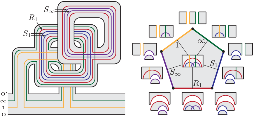
We reorganize the proof in [17] to fit it within our general framework of polytopes and identities . We use the notation for the lattice considered in [17]. The corresponding graph (in the sense of both and ) is the path of length three, yielding a pentagon of metrics whose sides correspond to , , , , and (where the left-hand notation is shorthand for the right-hand notation in the proof of Theorem 5.3). The auxiliary hypersurface is diffeomorphic to and cuts out from , leaving the cobordism with three boundary components.
Figure 9. At left, the half-dimensional diagram of the cobordism for the lattice . Note that is represented by two concentric curves, arising as the boundary of the tubular neighborhood of a circle representing the sphere (and similarly for ). At right, the pentagon of metrics, analogous to the hexagon in Figure 3.
Keeping the 3-periodicity in mind, we prove exactness by applying Lemma 6.1 with
where we have yet to define . The first condition of Lemma 6.1 is then satisfied by Proposition 5.6 with .
Let denote the edge of the pentagon corresponding to , considered as a one-parameter family of metrics on stretching from to . Viewing as a cobordism from the empty set to , with the family of metrics , we have components
In other words, these elements count isolated trajectories in moduli spaces of the form and . In fact, by Lemma 5.4 of [17], when the perturbation on is sufficiently small, there are no irreducible critical points and all components of the differential on vanish, as do and .
We define the maps exactly as before. We similarly define maps and which count isolated trajectories in :
We combine these components to define the map by
(28)
(31)
which is written out in full in Appendix II. The terms in (31) break on a boundary-stable critical point in . Of these, the term is singly boundary-obstructed, while the other two are compositions of a non-boundary obstructed operator and a doubly boundary-obstructed operator (see Definition 24.4.4 in [15]). Finally, we introduce the chain map defined by
(34)
where and . So the coefficient of in is a count of the zero-dimensional stratum of , over all such that is a summand of .
Furthermore, by Proposition 5.6 of [17], is a quasi-isomorphism. We conclude that is a quasi-isomorphism as well. This is precisely the second condition of Lemma 6.1, which then implies the theorem.
∎
Remark 6.3.
In fact, the authors of [17] show that the map induced by on is given by multiplication by the power series
The proof is related to that of the blow-up formula, Theorem 39.3.1 of [15].
Equation (35) is proved by counting ends. The maps and are defined using the vanishing elements and exactly as before. By analogy with the maps above, we also define vanishing maps and which count boundary points of . Finally, we define by
(38)
(41)
which therefore vanishes as well. The form of follows from the model case of Morse theory for manifolds with boundary, as described in Appendix I. Note that all the terms in (41) break on a boundary-stable critical point in . The term is singly boundary-obstructed, while the other four are compositions of a non-boundary-obstructed operator and a doubly-boundary-obstructed operator. In Appendix II, we have written out these terms in expanded form in order to verify the following lemma.
Lemma 6.4.
The map is equal to the component of from to :
Proof.
As in the proof of Lemma 4.7, all terms on the right appear exactly once on the left, with the additional terms on the left being those which do not have a good break on any . We divide these extra terms into those with
(i)
no break on ;
(ii)
a boundary-stable break on ;
(iii)
a boundary-unstable break on .
Terms of type (i) can be enumerated just as in the proof of Lemma 4.7, so each occurs twice in . Dropping indices where it causes no ambiguity, the terms of type (ii) occur in six pairs:
Finally, the terms of type (iii) occur in five pairs:
We conclude that terms of types (i) and (ii) are double counted by while those of type (iii) are counted once each by and . We therefore have equality over .
∎
Remark 6.5.
If we consider a boundary-unstable break on to be a good break as well, then Remark 4.8 goes through exactly as before. Furthermore, counts those trajectories which break well on (see also the discussion following Proposition 5.5 in [17]).
Remark 6.6.
For the lattice , we introduced the auxiliary hypersurfaces , , and in order to build the pentagon of metrics. The edges contribute vanishing terms to by Lemma 5.5, whereas the edge contributes the term . Thus,
and once more we can view (35) as a “generalization” of (5).
7. The link surgery spectral sequence: convergence
We are now positioned to identify the limit of the link surgery spectral sequence.
as the sum of all relevant components of the differential on the subcomplex
of . Then implies that is a chain map. Consider the filtration given by the weight of the last digits of . By applying the final assertion of Lemma 6.1 to the surgery exact triangles arising from the component , we conclude that induces an isomorphism between the pages of the associated spectral sequences.
Therefore, is a quasi-isomorphism, as is the composition
lattices of the form and give rise to filtered complexes;
(ii)
the lattice gives rise to an exact sequence.
We considered more general lattices in Theorem 5.3 and Proposition 5.6 in part to make clear how both these facts arise as special cases of the same polytope constructions. The lattice will arise naturally in Section 8.
7.1. Grading
The group is endowed with an absolute mod 2 grading , as explained in Sections 22.4 and 25.4 of [15]. This gradings is uniquely characterized by two properties. First, the group is supported in even grading. Second, if is a cobordism from to , then the map shifts according to the parity of the integer
(43)
where is the Euler number and is the signature of the intersection form on .
Note that is additive under composition, since both the signature and Euler characteristic are additive in this context. Furthermore, if parameterizes an -dimensional family of metrics on , then the map shifts by .
We now introduce an absolute mod 2 grading on the hypercube complex which reduces to in the case . In fact, it will be useful to define on the larger complex associated to the lattice . Let be homogeneous with respect to the grading. Then for , we define
(44)
Here the subscripts and are shorthand for the initial and final vertices of .
Lemma 7.2.
The differential on and lowers by 1.
Proof.
Since is defined using a family of metrics of dimension on , it shifts by
The gradings and coincide under the quasi-isomorphism
defined in .
Proof.
The weight of the vertex is . Therefore, given , by (44) we have
So it suffices to show that the quasi-isomorphism lowers by . But is a composition of maps , each of which is a sum of components of . So we are done by the Lemma 7.2.
∎
7.2. Invariance
The construction of the hypercube complex
depends immaterially on numbering the components of , and materially on a choice of regular metric and perturbation on the full cobordism , where the metric is cylindrical near each of the hypersurfaces . Let and be two such choices.
Theorem 7.4.
There exists a -filtered, -graded chain homotopy equivalence
which induces a -graded isomorphism between the associated pages for all .
Proof.
We start by embedding a second copy of each in as follows (see Figure 10 for the case ). First, relabel the incoming end as and every other as . Then embed a second copy of , labeled , just above the original. Finally, embed a second copy of each , labeled , just below the original. We now have an embedded hypersurface for each in the hupercube , with diffeomorphisms
(45)
(46)
where in (46) we assume . Furthermore, and are disjoint if and are ordered.
Figure 10. At left, we have the half-dimensional diagram of the cobordism used to prove analytic invariance in the case . For each , the hypersurfaces (in blue) and (in red) bound a cylindrical cobordism. At right, we can fix the blue metric on (top), or the red metric on (bottom). The green metric on the middle rectangle represents an intermediate state. To construct the homotopy, we slide the metric from that on the top rectangle to that on the bottom rectangle in a controlled manner, as explained in Figure 11.
Our strategy is as follows. We define a complex
where the differential is defined as a sum of components
Those components of the form are inherited from . So we may view as the complex over obtained from quotienting by the subcomplex over . The component is induced by the cobordism over a family of metrics and perturbations parameterized by a permutohedron , to be defined momentarily. Then implies that
is a chain map. If we extend the grading verbatim to , then is odd as a map on by Proposition 7.3, and thus even as a map from and . Thus, is -graded, and it is clearly -filtered. By (45), the map
induces an isomorphism on homology. Thus, filtering by the horizontal weight defined by , induces a -graded isomorphism between the pages of the corresponding spectral sequences. By Theorem 3.5 of [19], we conclude that induces a -graded isomorphism between the pages for each . Thus, is a quasi-isomorphism, and therefore (since we are working over a field) a homotopy equivalence.
It remains to construct the family parameterized by each and to prove that . We start by fixing a metric on each cylindrical cobordism for which and (we proceed similarly with regard to the perturbations, though we will suppress this). Here the notation denotes the restriction of to . The point is defined to correspond to the metric . Now for each , we specify a metric on by its restriction to each of three pieces:
We will use these metrics to construct the family parameterized by in several stages. The case is illustrated in Figure 11.
Figure 11. The hexagon is drawn so that increasing the vertical coordinate is suggestive of moving from the red metrics to the blue metrics. Gray represents the cylindrical metrics , while green represents an intermediate mixture of red, blue, and gray.
We first describe a family of non-degerate metrics on , parameterized by the permutohedron . Let denote the facet of corresponding to the internal vertex . may be obtained from by subdividing each facet by the ridge . In the case, this amounts to adding a vertex at the midpoint of each vertical edge in a square. In the case, shown at right in Figure 16, we have cross the hexagon with an interval and add an edge to each lateral face. We next label the facets and by and , respectively. Furthermore, we label and by and , respectively.
We then associate the metric to each vertex of lying on . The remaining vertices of lie on or . We associate to these vertices the metrics and , respectively (note that and ). At this stage, we have defined on the 0-skeleton of . We proceed inductively: having extended to the boundary of a k-dimensional face of , we extend to the interior of , subject to the following constraint:
(47)
If is constant over some hypersurface or component of , then so is .
In particular, the family is constant when restricted to each of the facets and and each of the ridges .
The family over slides the metric (and perturbation) on in stages (in Figure 11, is the inner hexagon). We now extend to a family which incorporate stretching. To each facet of , we glue the polytope along the facet (in Figure 11, these are the six lightly shaded rectangles). We extend over by stretching on in accordance with the latter coordinate (recall that the metric on is constant over ). Next, along each ridge in , we glue on the polytope in the obvious manner (in Figure 11, these are the six heavily shaded squares). The first interval parameterizes stretching on while the second interval parameterizes stretching on . We continue this process until the last stage, when we glue one cube at each vertex of , over which stretches on the corresponding maximal chain of internal hypersurfaces.
In the end, we have simply thickened the boundary of to describe a family of metrics on parameterized by the permutohedron (the full hexagon in Figure 11). This family is degenerate over the boundary of precisely as described by Proposition 2.4. Now, for each , we construct a family of metrics over by restricting the family to over an appropriate face of (here the constraint (47) is essential).
The proof that now lifts directly from the original proof that , with one new point that we now explain. The component of from to vanishes if and only if
(48)
Consider the composite map corresponding to the family over the facet of . Since the family over the corresponding facet of is constant, the only sections of the facet which contributes non-trivially to this map are those of the form in the boundary of the cubes (in Figure 11, these are the two segments of the top edge of the hexagon which lie in the boundary of the heavily shaded squares). The other sections cannot give rise to 0-dimensional moduli spaces, since they involve at least one parameter which does not change the metric. We can therefore identify the map associated to the facet with (in Figure 11, we are contracting out the middle segment of the top edge). Similarly, the map associated to the facet coincides with , and the sum on line (48) coincides with the map associated to the remaining lateral facets of . Thus, the full equation expresses the fact that the map associated to the full permutohedron is a null-homotopy for the map associated to its boundary. The other components of vanish by a completely analogous argument.
∎
Remark 7.5.
Recall the top and bottom rectangles at right in Figure 10. Suppose that the red and blue metrics agree where they overlap, so that the family on can be made completely constant. Then only the cubes contribute non-trivially to the map . Discarding the rest of and gluing these cubes together, we build a permutohedron giving rise to the same map. This viewpoint highlights the connection between the permutohedra and the permutohedra that we first constructed in Section 2, using only cubes which stretch the metric along maximal chains of internal hypersurfaces.
8. The map and
Given a cobordism , Kronheimer and Mrowka construct a map . In [15], this map is defined by pairing each moduli space with the first Chern class of the natural complex line bundle on . A dual description of the map is given in [17]. We will use the notation for this map on the chain level.
We introduce a third description which fits in neatly with our previous constructions. We first recall some facts about the monopole Floer homology of the 3-sphere (see Sections 22.7 and 25.6 of [15]). With round metric and small perturbation, the monopoles on the 3-sphere consist of a single bi-infinite tower of reducibles, with boundary-stable if and only if , and . Furthermore, sends to , and in particular, is non-zero if and only if . It is this last property which motivates the following reformulation.
Given a cobordism , let denote the manifold obtained by removing a ball from the interior of and attaching cylindrical ends to all three boundary components, with the new end regarded as incoming. Choose the metric and perturbation on so that we return to the situation described in the last paragraph over . We define the map by replacing each moduli space in the definition of with the moduli space . In other words,
One sees that is a chain map and well-defined up to homotopy equivalence by the same argument used for , together with the fact that there are no isolated trajectories from to any other . Note that the choice of ball in may be interpreted as a metrical choice, since a diffeomorphism of sending one ball to another is an isometry from to .
Proposition 8.1.
The map is homotopy equivalent to the map .
Proof.
Given a cobordism , we may assume the cochain representing is supported over the configuration space of a small ball. The homotopy relating the two maps is now given by stretching the metric normal to the 3-sphere bounding this ball.
∎
This justifies a return to the notation .
We now define a fourth version of monopole Floer homology, denoted and motivated by the properties of in Heegaard Floer homology. We use the shorthand for the map induced by the cylindrical cobordism, with some regular choice of metric and perturbation (which need not have the same restrictions on both ends).
The complex is defined to be the mapping cone of :
Since is an even map, the differential is odd, and therefore naturally extends to (as does for torsion spinc structures). We then define as the homology . While the completion involved in the definition of the other versions has no effect here, we keep the bullet for notational consistency. We will see that describes a functor in the same spirit as . By construction, there is an exact sequence
(49)
of modules where acts by zero on . Here the maps and are even, while is odd.
The construction of the map induced by a cobordism is essentially the same as the case of the spectral sequence to follow, but we describe it separately for concreteness and to motivate what follows. First fix a small ball in the interior of (which we subsequently excise). We relabel the ends of as and and embed a second copy of each in the interior of as follows (see Figure 12a). Consider a path in from to such that a small tubular neighborhood of the path contains the ball. is obtained by taking a parallel copy of just inside the boundary and smoothly pushing the region in past the ball, so that cutting along leaves the ball in the first component . Similarly, is obtained by taking a parallel copy of near the boundary and smoothly pushing the region inside inward past the ball, so that cutting along leaves the ball in the second component . Note also that both and are diffeomorphic to .
Figure 12. Surface represents the cobordism used in the construction of the chain map . Surface represents the cylindrical cobordism used to prove that is well-defined, as discussed at the end of this section.
The intersection of and is modeled on , so we can choose the metric on to be cylindrical near both interior hypersurfaces. Consider the interval of metrics which stretches from to . We use this interval to define eight operators which count isolated trajectories in the moduli space
where
and
We then define by the same expression as in (19), except that if ends in and ends in , then is replaced by So in full, we have
From this perspective, the differentials on and are
respectively.
Finally, the map is defined by
We now turn to the general construction of the total complex underlying the version of the link surgery spectral sequence. In this section, we will denote this complex by , though in other sections we will return to the notation when it is clear from context which version is intended. The same goes for the pages etc.
Given an -component framed link , we embed a small ball in the interior of , centered at a point . Next we relabel the incoming end as and every other as . We then embed a second copy of , labeled , just above the first, modified so that it now passes above the ball. Finally, we embed a second copy of each , labeled , just below the first, modified so that it now passes below the ball, using the path as a guide. See Figure 13 for the case . We now have an embedded hypersurface for each . Furthermore, the intersection data is precisely what we expect for this hypercube, namely that intersects if and only if and are not ordered. Therefore, given any we may construct a family of metrics on parameterized by a permutohedron of dimension .
Figure 13. At left, we have the half-dimensional diagram of the cobordism with a small ball removed in the case . For each , the pair and bound a cylindrical cobordism containing the ball. At right, we have drawn the corresponding hexagon so that increasing the vertical coordinate is suggestive of translating the sphere through . The small figures at the vertices and edges illustrate the metric degenerations, read as composite cobordisms from left to right. In each, the component containing the sphere is more heavily shaded.
Now fix a regular metric and perturbation on the cobordism which is cylindrical near every hypersurface and round near . We will define a complex
(50)
where the differential is the sum of components over all . We have set things up so that the ball is contained in if and only if ends in and ends in . So when and end in the same digit, the operators may be defined exactly as before (see (16)). In the other case, we construct operators using moduli spaces which are defined by slightly modifying the definition of the moduli spaces . Namely, if is in the interior of the face , with the last digit changing between and , then an element of is a -tuple
as before except that
Let be synonymous with if and end in the same digit, and with otherwise. Similar remarks apply to and .
We then define by precisely the same expression as (19), with each underlined.
The proof that goes along familiar lines. The operators may be defined exactly as before when and end in the same digit. When ends in and ends in , we define operators which count ends of 1-dimensional moduli spaces , which in turn are defined by slightly modifying the definition of the moduli spaces in the same manner as above. As before, these operators all vanish. Now let be synonymous with if and end in the same digit, and with otherwise. Similar remarks apply to and . We then define by precisely the same expression as (23), with each and underlined.
Lemma 8.2.
is equal to the component of from to :
Thus, is a differential.
Proof.
Recall that is an unstable reducible and that there are no isolated trajectories from to any other . It follows that 1-dimensional moduli spaces have the same types of ends as , as described in Lemma 4.3. Similarly, has the same types of ends as . Now we simply repeat the proof of Lemma 4.7 with everything underlined.
∎
Remark 8.3.
The case shows that is a chain map. The case shows that is a chain map when an elementary 2-handle cobordism, and goes through without change for arbitrary cobordisms.
In order to interpret Lemma 8.2 as a result in hat theory, we collapse
along the final digit, with given by the sum of maps where
(53)
Define the horizontal weight of a vertex to be the sum of all but the final digit. Filtering by , we obtain the version of the link surgery spectral sequence. In particular,
and the differential is given by
In order to identify with , we expand to the larger complex
(54)
where we have again relabeled the and embedded a second copy of each which passes on the opposite side of the ball. These hypersurfaces all avoid the auxiliary hypersurfaces which are confined in the handles. The intersection data is as predicted for the shape of the lattice by Theorem 5.3, so we may build families of metrics parameterized by graph associahedra which define maps and . The auxiliary hypersurfaces still cut out , so the corresponding facets contribute vanishing operators as before. We conclude from 8.2 that forms a complex.
Finally, we turn to the surgery exact triangle. Recall the hypersurfaces , , , and auxiliary , , and . After relabeling, these become , , , , , , and , to which we add , , , and . The nine hypersurfaces in the interior of intersect as predicted by the shape of the lattice , yielding the graph associahedron on a chain of length , namely, the 3-dimensional associahedron , shown in Figure 14.
Figure 14. The lattice corresponds to Stasheff’s polytope, drawn at center and right so that the depth coordinate is suggestive of translating the sphere through . Recall that the same polytope is associated to the lattice in Figure 5, redrawn at left. In fact, by Theorem 5.3, an associahedron arises whenever the lattice is a product of at most two chains. The map corresponding to above is a null-homotopy for the sum of the maps associated to the faces. Those associated to and vanish as before, leaving a nine-term identity on the chain level.
The map associated to is given by the same expression as , but with and , over the one-parameter family of metrics stretching from to . This gives the identity
(55)
where and are the analogues of corresponding to the four hypersurfaces ending in and , respectively, together with , , and . Similarly, is modeled on the expression (41) for and includes terms counting monopoles on cobordisms with four boundary components. By the same reasoning as in the proof of Lemma 8.2, the analogue of Lemma 6.4 goes through essentially unchanged (although with nearly twice as many terms), leading to the nine-term identity given by the lower left entry of
The upper left and lower right identities are precisely those given by Lemma 6.4. Rewriting this identity via (53), we have the analog of (35):
The final map is a chain map by (55). Filtering the corresponding square complex
by the second digit, and recalling that and are quasi-isomorphisms, we conclude that . Therefore, is a quasi-isomorphism as well. Now exactly the same algebraic arguments yield the surgery exact triangle, and more generally the full statement of the link surgery spectral sequence, for .
The grading and invariance results of Section 7 readily extend to by viewing the underlying complex in terms of as in (50) and (54). In this way, we may extend to a mod 2 grading on using the same definition. Since cuts down the dimension of moduli spaces by two, the maps on obey the same mod 2 grading shift formula as the maps on . In particular, Lemmas 7.2 and 7.3 still apply, and when , and coincide on . The proof of Theorem 7.4 regarding invariance also readily adapts to a version for , using a cobordism with hypersurfaces (that is, two copies of each hypersurfaces in Figure 13), where we maintain the round metric on the boundary of the ball throughout. The case is pictured in (b) of Figure 12, and implies that is well-defined. Similarly, the case for a general cobordism implies that is well-defined. The composition law (2) follows from the case by stretching from to .
8.1. Realizations of graph associahedra
Recall the pentagonal realization of Stasheff’s polytope at center in Figure 14, and the inductive realization of as a refinement of in the proof of Theorem 7.4. Both of these realizations are motivated by the “sliding-the-point” proof of the naturality of the action in Floer theory (though from our perspective we are sliding the sphere). To see why, recall that to any product lattice we may associate a map whose longest component counts monopoles on over a family of metrics parameterized by a polytope (see Remark 5.4). We then expect the longest component of the homotopy which expresses the naturality of the action with respect to to count monopoles over a family of metrics parameterized by , where the latter coordinate slides the sphere through (see Figure 15). In Section 8, we instead embedded two copies of each hypersurface in , because this approach fit more cleanly with our earlier constructions.
Figure 15. At left, we slide the sphere through the full cobordism from Figures 2 and 3. Each time the sphere crosses an embedded hypersurface, we add a ridge to the corresponding lateral facet of . Once the sphere has completed its journey, we have a realization of . At right, we similarly slide the sphere through the full cobordism from Figure 9, adding ridges to . Once the sphere has completed its journey, we have .
More generally, consider any realization of the graph associahedron of dimension associated to a lattice . We may realize the graph associahedron associated to as a refinement of . Namely, for each internal vertex of , we add a ridge at height to the corresponding lateral facet of . We ignore auxiliary hypersurfaces, as the sphere never passes through them. In the two cubical realizations below, we have applied this construction twice, starting from a graph associahedron which is geometrically an interval.
Figure 16. Two alternative realizations of the permutohedron from Figure 4, and one of the graph associahedron from Figures 6 and 7.
Note that the lattices and both correspond to the graph consisting of a path of length . By the above remarks, this fact yields a simple realization of the associahedron by adding ridges to . We obtain a similar realization of each permutohedron from the fact that . If we build these realizations inductively, starting from the point, then each is naturally a refinement of the hypercube (see Figure 17), and we may arrange that refines as well. Upon sharing these realizations with experts, we were directed to similar ones in [27], which also refine hypercubes but have vastly different origins. For as a convex hull, see [18] and [8].
Figure 17. We realize by adding ridges with integral vertices to the facet of the hypercube . Similarly, is obtained by adding ridges to the hypercube.
9. Khovanov homology and branched double covers
We now turn to the construction of the spectral sequence from to in Theorem 1.3. We would like to interpret the page as the result of applying a much simpler functor than to the branched double cover of the hypercube of resolutions. To this end, we prove the and analogs of Proposition 6.2 in [24].
Proposition 9.1.
Let . Then, is a rank one, free module over the ring
generated by some class , and entirely supported over the torsion spinc-structure. Moreover, if is a curve which represents one of the circles in one of the summands, then the three-manifold is diffeomorphic to , with a natural identification
Under the cobordism induced by the two-handle, the map
is specified by
(56)
where here is some fixed generator of , and is any element of . Dually, if is an unknot, then , with a natural inclusion
Under the cobordism induced by the two-handle, the map
is specified by
(57)
where here is a generator in the kernel of the map .
Proof.
The description of holds whenever has a metric of strictly positive scalar curvature, as shown in Proposition 36.1.3 of [15]. Note also that, by Theorem 3.4.4 of [15], the maps and behave naturally with respect to the above module structures.
We first consider the case where represents a circle in one of the factors. As is null-homologous in , we have
On the other hand, since , the corresponding surgery exact triangle splits (by comparing the ranks) as
Therefore, is surjective, which together with naturality, forces (56).
Now suppose is an unknot. As is null-homologous in , we have
So the image of is contained in . Now and the short exact sequence reads
Therefore, is injective, which together with naturality, forces (57).
∎
Corollary 9.2.
Let . Then, is a rank one, free module over the ring . After removing from (56) and (57), Proposition 9.1 holds for .
Proof.
The map is surjective on the level of homology, so we have the short exact sequence
In particular, is identified with , which is the image of under the action of . Under this identification, the map coincides with the restriction of to . The same holds in the case of .
∎
We now construct the spectral sequence associated to a link . We first fix a diagram with crossings. Following Section 2 of [24], we associate to a framed link to which we will apply the link surgery spectral sequence. First, in a small ball about the crossing , place an arc with an end on each strand as shown in the resolution of Figure 18. Each of these arcs lifts to a closed loop in the branched double cover , giving the components of a link . Note that all of the resolutions of agree outside of the union of the . Furthermore, the branched double cover of over the two unknotted strands of is a solid torus, with meridian given by the preimage of either of the two strands pushed out to the boundary of . So for each , we may identify with .
In this way, for each crossing , we obtain a triple of curves ( in the corresponding boundary component of , which represent meridians of the fillings giving the branched covers of the 0-, 1-, and -resolutions at , respectively. In this cyclic order, the curves may be oriented so that the algebraic intersection number of consecutive curves is +1. We change this to by flipping the orientation on the branched double cover (whereas in [24] this is done by replacing with its mirror). In the language of [24], each triple forms a triad. From our 4-manifold perspective, this is precisely the condition that each 2-handle in a stack is attached to the previous 2-handle using the -1 framing with respect to the cocore (see the discussion preceding Theorem 4.11). From either perspective, framing by , we are in precisely the setup of the link surgery spectral sequence, with for all . Now, using Corollary 9.2, the argument in [24] may be repeated verbatim to show that the complexes and are isomorphic, and therefore that is isomorphic to .
Figure 18. We have one short arc between the two strands near each crossing, in both the original diagram and its resolutions.
As an alternative to the argument in [24], we now present a more global description of the isomorphism , taking advantage of the construction in [3] of a framed link (there denoted ) which gives a surgery diagram for the branched double cover . Note that our convention in [3] on the orientation of surgery diagrams is precisely the opposite of the more sensible one we are using now (in this paper, the branched double cover of the right-handed trefoil is given by +3 surgery on an unknot, and we plan to revise [3] accordingly). This construction of is illustrated in Figure 19 for the standard diagram of the right-handed trefoil . We first fix a vertex for which the resolution consists of one circle. The link is obtained as the preimage of the corresponding red arcs in Figure 18, where the component is given the framing . Note that the link is represented in this surgery diagram by the framed push-off of .
Figure 19. At left, we number the crossings in a diagram of the right-handed trefoil . The resolution has one circle, and one (arbitrarily-oriented) arc for each crossing. We then cut the circle open at the dot and stretch it out to a line, dragging the arcs along for the ride. Reflecting each arc under the line yields the framed link and linking matrix at right. Surgery on gives , which is the lens space .
For each , let be the link with framing modified to
on . Then gives a surgery diagram for , where the resolution consists of circles. This is illustrated in Figure 20 for the trefoil . Furthermore, each elementary 2-handle cobordism is given explicitly by 0-surgery on either or its meridian , in the case where or , respectively. Here is the saddle-like surface cobordism from to .
Figure 20. Continuing from Figure 19, above we obtain the cube of surgery diagrams for the right-handed trefoil . All solid components are 0-framed, while all faded components are -framed.
The link surgery cube of 3-manifolds and 4-dimensional 2-handle cobordisms above is the branched double cover of the Khovanov cube of 1-manifolds and 2-dimensional 1-handle cobordisms below. At the upper right of each box, we record the associated numerical data, which determines as described in [3] and Remark 9.3 below. The orientation conventions for odd Khovanov homology are also described in [3], but over these orientations are irrelevant.
Motivated by Corollary 9.2 and Figure 20, we define a complex with underlying -vector space
and differential given by the sum of maps over all immediate successors in . These in turn are defined by
The central point of [3], reduced mod 2, is that we can take the complex as the definition of . Namely, is precisely the version of defined at the end of Section 3, using the identification of with at the end of Section 4.
There, the main tool is to present each group by the linking matrix of , using the common basis given by the meridians .
On the other hand, Corollary 9.2 immediately implies that is isomorphic to the page of the link surgery spectral sequence for . We conclude that and are isomorphic complexes, and therefore that is isomorphic to as an -vector space. This establishes Theorem 1.3.
Remark 9.3.
In [3], we show that the framed isotopy type of is completely determined by the linking matrix of . If follows that the pages for are determined by as well (up to an overall shift in bigrading that depends on ). In fact, since we are working with coefficients, the orientations of the arcs (and corresponding components of ) are extraneous as well. We need only record which pairs of arcs in are linked, as well as itself. On the other hand, the matrix with signs fully encodes the odd Khovanov homology of with coefficients (again, up to an overall shift in bigrading that depends on ), and should also encode a lift of the spectral sequence to .
9.1. Grading
For the duration of this paragraph, we return to the notation to distinguish the version of the spectral sequence from the version. Our goal is to relate the mod 2 grading on to the integer grading on . Since is surjective on , may be identified as a -graded vector space with the kernal of the map
This permits us to work with the grading on instead.
Let be an oriented link and fix a diagram with crossings. Let and denote the number of positive and negative crossings, respectively. Consider the hypercube complex given by surgeries on . Recall that when the resolution consists of circles.
We may think of a generator as an element of either or . The group is supported over the torsion spinc structure, and a short calculation shows that , where is the rational grading over the torsion spinc-structure, defined in Section 28.3 of [15]. Moreover, on we have
(58)
Recall that has a quantum grading and a homological grading . The -grading is defined as the linear combination . Translating from the definitions in [22], we may express these gradings as
Here and denote the number of positive and negative crossings in . The final formula defines a function .
We next define a function which lifts the mod 2 grading on . Note that all cobordisms over the hypercube satisfy . This is easily seen for an elementary cobordism, and follows in general from signature additivity. Using (43) and (44), we have
The last line follows from Lemma 9.4 below. Reducing mod 2, we have the first claim of Theorem 1.3.
For the remaining claim about the determinant, note that
where denotes the Jones polynomial of (when , everything vanishes). Alternatively, one can show that the number of spinc structures on is and that
is one when , and vanishes otherwise.
∎
Lemma 9.4.
The signature and nullity of are given by
Proof.
The nullity is sometimes defined as the nullity of any symmetric Seifert matrix for , and sometimes as . These definitions are equivalent since presents .
We will prove the formula for by relating to the signature of a certain 4-manifold bounding . Recall that the diagram has a checkerboard coloring with infinite region in white. The black area forms a spanning surface for with one disk for each black region, and one half-twisted band for each crossing. View as in the boundary of , and push into the interior. We then define as the branched double cover of over . In [12], Gordon and Litherland show that the intersection form of is the Goeritz form associated to , and that
where (see Figure 21). The minus sign in front of is due to the fact that the signature convention in [12] is the opposite of ours. Using the relations
we can also express as
Therefore,
(59)
Figure 21. Four types of crossings in an oriented diagram with checkerboard coloring. The letters , , , and denote the number of crossings of each type.
We now construct a Kirby diagram for (see Section 3 of [24] and Section 3 of [13] for similar constructions). First, form the black graph resolution by resolving each crossing so as to separate the black regions into islands (that is, 1-resolve a crossing if and only if it is of type or in Figure 21). Draw a 1-handle in dotted circle notation along the boundary of each black region in . Next, add a 2-handle clasp at each crossing, with framing if the crossing is of type or , and otherwise. Finally, delete one of the 1-handles.
Since vanishes, signature additivity implies .
Next we construct a relative Kirby diagram for the cobordism . First turn all but one of the circles in into 1-handles to get a surgery diagram for , regarded as the incoming end of . Next, introduce a 0-framed clasp at each of the crossings corresponding to 0 digits of . This gives a relative Kirby diagram for the cobordism . Finally, introduce -1 framed clasps at each of the remaining crossings, and -1 framed meridians on each of the 0-framed clasps. This gives a relative Kirby diagram for the cobordism . After pulling off and blowing down all of the -1 framed meridians, and filling in the incoming end with a boundary connect sum of copies of , we recover the Kirby diagram for . Therefore,
Recall the construction of the surgery diagram for , as in Figure 19. Let be the 4-manifold obtained by attaching 2-handles along . By construction, bounds . Just as in the above proof, a Kirby diagram argument shows that
where is the linking matrix of , which is congruent to the linking matrix of the arcs in Proposition 1.7. From Lemma 9.4, we arrive at the formula
Furthermore, since presents .
∎
Example 9.5.
Consider the resolution of the right-handed trefoil in Figure 19, with given by the linking matrix at right. The signature formula gives
For the mirrored diagram representing the left-handed trefoil , consider the mirrored resolution . Now the signature formula gives
9.2. Invariance
We now turn to the proof of Theorem 1.4, which describes the extent to which the spectral sequence depends on the choice of diagram for the link L.
Let and be two diagrams of the link . Let represent the hypercube complex associated to diagram , for some choice of analytic data (which we may suppress by Theorem 1.2). The goal is to construct a filtered chain map
which induces an isomorphism on the page, and therefore on all higher pages as well. It suffices to consider the case where and differ by a single Reidemeister move.
In [2], Baldwin defines such a map for each of the three Reidemeister moves. While he was considering the Heegaard Floer version of the spectral sequence, his maps have direct analogues in the monopole Floer case. The difficult part is proving that induces a homotopy equivalence from to on the page. However, this argument only involves properties of the Khovanov differential, drawing heavily on the proof that Khovanov homology is a bigraded link invariant (see [22]). It is also clear from the construction that preserves the bigrading on Khovanov homology, and therefore .
Now, suppose links and are related by a mutation. Fix diagrams and for and which exhibit the mutation. Let and be the associated framed links in , and let and be the associated framed links in and . In Section 4 of [3], we prove that there is an orientation-preserving diffeomorphism
for which and are isotopic as framed links. This implies that there is an orientation-preserving diffeomorphism
for which and are isotopic as framed links. Appealing to Theorem 1.2, we conclude that the pages of the spectral sequences associated to and agree for all .
∎
9.3. The spectral sequence for a family of torus knots?
In order to illustrate the spectral sequence in action, we now present an example which is both highly speculative and, we hope, compelling. Consider the family of torus knots given by
For this family, the unreduced Khovanov homology with coefficients in takes the form of repeating blocks, and is stable, up to a shift in quantum grading, as grows [29], [31]. Computing explicitly for several values of using Bar-Natan’s KnotTheory package [1], a similar pattern of repeating blocks emerges, as shown in Figure 22. Surely this pattern persists and can be deduced by similar techniques. Up to a shift in quantum grading, we have inclusions
Conjecture 9.6.
For each such torus knot, and some choice of analytic data and diagram, the higher differentials are as shown in Figure 22. In particular, the spectral sequence converges at the page, and the above inclusions on the page extend to the and pages.
Figure 22. Each dot represents an summand of in the -plane. The diagonal is heavily shaded and the diagonal is lightly shaded (unless ). The and differentials are in red and blue, respectively, as are their victims. The surviving (black) dots generate . The shaded diagonals also correspond to and . For , there is precisely one black dot on each diagonal in this range, giving the expected rank of in each grading.
One intriguing way to frame this conjecture is as follows. Using the -bigrading in Figure 22, we may define higher -polynomials by
for each . Then Conjecture 9.6 implies that the -polynomials on the and pages are monic monomials, while
(60)
Here denotes Rasmussen’s -invariant. Based on Theorem 1.5, we suspect that these polynomials are highly relevant to the connection between Khovanov homology and Floer homology. It would be very interesting to compare (60) with the polynomials arising from Greene’s conjectured -grading on , defined in Section 8 of [13].
Our primary evidence for Conjecture 9.6 comes from [2], where Baldwin deduces that the Heegaard Floer spectral sequence for is as shown in Figure 22. His argument uses the Khovanov and Heegaard Floer contact invariants to show that the lower left generator survives to for every torus knot. This is the only survivor in the case of , as the branched double cover is the Poincaré homology sphere. Alas, we have not rigorously computed the monopole Floer spectral sequence even in this case, since for now we lack an analogous contact invariant.
As further evidence, we cite the compatibility of with the page implied by our conjecture. The branched double cover of is the Brieskorn integer homology sphere
which arises by Dehn surgery on a trefoil knot. Using a surgery exact triangle, the Heegaard Floer groups are explicitly calculated in [23]. The same techniques should apply in the monopole case, and using (49), we expect that
where the subscript denotes grading (see also [21]). In particular,
We also expect that, for some choice of metric and perturbation, the first summand arises from the reducible generator of in lowest grading, while each pair of summands in parenthesis arises from a single irreducible generator. Comparing with Figure 22, we imagine that the reducible is sitting in the lower left corner, whereas the pairs arising from each irreducible are in adjacent homological grading and grading. In particular, the grading on is compatible with the grading on , as required by Theorem 1.5.
For links such that the bigrading on the higher pages is well-defined, we may encode the higher pages of the spectral sequence in the form of a 2-variable higher Khovanov polynomial, given by
for each . We then obtain higher Jones polynomials, given by
for each . The ordinary Jones polynomial coincides with . Furthermore, if is quasi-alternating, then for all .
We now record in full the various higher polynomials associated with the differentials in Figure 22, in order to provide a (conjectural) data-set to aid in the search for a combinatorial description. For comparison, we include the polynomials on the page as well. Note that the optimal input for an algorithm may not be a diagram of the link itself, but rather the arc-linking data which encodes the mutation equivalence class, as described in Remark 9.3.
Conjecture 9.7.
Let and let . Set
For each , the higher Khovanov polynomials are given by
The higher Jones polynomials are given by
The higher -polynomials are given by
Here , , and . So both and may be expressed as
10. From pseudoholomorphic polygons to associahedra of metrics
This section is intended for those readers interested in the relationship between monopole Floer homology and Heegaard Floer homology (or more broadly, gauge theory and Lagrangian intersection theory). In the former, the identities arising from permutohedra encode the fact that the Floer chain maps associated to 2-handle additions commute up to homotopy. In the latter, we have relations which encode associativity up to homotopy (say, for the Floer maps associated to a stack of 2-handles). The relations arise from associahedra, which naturally compactify the space of conformal structures on polygons (see, for example, Section 2 of [2]). We now outline an alternative construction of the hypercube complex that is modeled closely on the version in Heegaard Floer homology [24]. In particular, the components of the differential will be built using only associahedra of metics.
Let be an -component, framed link. By a standard construction starting with a Heegaard multi-diagram subordinate to a bouquet of the link , we fix a Heegaard diagram for each with (see Section 4 in both [24] and [25], keeping in mind Remark 4.12). Fix vertices and let be the set of all paths from to . Fix a path given by . We now give an alternative construction of the cobordism with respect to the path .
Let denote the handlebodies associated with and let denote the regular polygon with edges . We thicken these handlebodies, glue them onto , and smooth the corners over the vertices of to obtain a smooth, oriented cobordism with boundary components (compare with Section 2.2 of [25]):
We have one embedded hypersurfaces in for each pair of handlebodies. The Heegaard diagram represents the internal hypersurface , which we also denote by . The Heegaard diagram represents an auxiliary hypersurface which is diffeomorphic to a connect sum of the form . Furthermore,
After filling in each auxiliary boundary component of with a connect sum of the form , we recover precisely the cobordism . In Figure 23, we have depicted this construction for the six paths in the hypercube .
Figure 23. We have one depiction of for each of the six paths from to in . The regions that result from filling in the auxiliary boundary components are heavily shaded. Conditions (i) and (ii) say that the (hypersurfaces associated to) arcs in distinct diagrams coincide in if and only if they have the same ends. The internal hypersurfaces are colored consistently with Figures 2 and 3. The hexagon from Figure 3 is built using the six squares of metrics that stretch on pairs of corresponding colored arcs in Figure 23. The remaining 24 squares cancel in pairs, in the sense of Proposition 10.1 below.
We embed the full set of internal hypersurfaces in as before, as well as an auxiliary hypersurface for all with , so that:
(i)
is identified with whenever has .
(ii)
is identified with whenever the subpath runs from to .
(iii)
The collection of hypersurfaces
associated to any particular intersect as suggested by Figure 23.
When and , we have constructed the full cobordism . Fix an initial metric and perturbation on , and on each by restriction. The intersection data required by (iii) corresponds to the lattice in Theorem 5.3. Degenerating the metric along a hypersurface mirrors degenerating the conformal structure on the polygon along the corresponding arc. So for each , we have an associahedron of metrics on . We define to be the map associated to , and then
by
Finally, the map is given by the sum of the over all pairs .
We now show that by considering the relations arising from the associahedra (this is analogous to the approach in [24]). Note there will be no terms corresponding to pinching off bigons, since we have effectively placed the generating cycle on each by filling it in. We let be the operator associated to the facet in . Using the appropriate end-counting map , we obtain the relation
since the innermost sum has an even number of terms, which are identical by (ii). Here, denotes the concatenation of the three paths. We conclude that .
In fact, we have reproduced the maps associated to the permutohedra :
Proposition 10.1.
Using the same choice of initial metric and perturbation on , we have
Proof.
Let . Each of the associahedra contains a single cube which stretches on internal hypersurfaces . These cubes are exactly those we glued together to form in Section 2. The remaining cubes in the associahedra fall into equivalence classes of even size, where two cubes are equivalent if they parameterize identical families of metrics on . Thus, their total contribution to is zero.
∎
The map analogous to in [24] counts pseudo-holomorphic polygons in the Heegaard multi-diagram where the conformal structure on is allowed to vary. Figure 23 directly illustrates how the space of conformal structures on corresponds to an associahedral family of metrics on . Conversely, the maps associated to permutohedra of metrics do not have direct analogues in Heegaard Floer homology. Of course, this did not prevent Ozsváth and Szabó from deriving their version of the link surgery spectral sequence. In order to prove that is a differential, they essentially used the above algebraic cancellation, in place of the geometric cancellation implicit in excising the duplicate cubes and gluing together what remains. We hope that the reader familiar with [24] has gleaned new intuition from access to a more expansive repository of polytopes.
Appendix I: Morse homology via path algebras
Monopole Floer homology may be viewed as an infinite dimensional version of Morse homology for manifolds with boundary. For a beautiful treatment of the finite dimensional model, see Section 2 of [15]. We now give a brief presentation of its essential features, assuming familiarity with Morse homology for closed manifolds. By recasting the combinatorics in terms of path algebras, we hope to illuminate the classification of ends in Lemma 4.3 and the form of the matrices (19), (23), (31), (34), and (41) used to define , , and .
Consider a manifold with boundary, equipped with a Morse function whose gradient is everywhere tangent to the boundary. The critical points in the boundary are classified as stable or unstable, according to whether the flow in the normal direction is toward or away from the boundary, respectively. We denote interior, boundary-stable, and boundary-unstable critical points by , , and , respectively. Note that interior gradient trajectories always flow from or to or , whereas boundary trajectories flow from or to or . We distinguish between interior and boundary trajectories from to , so there are eight types in all.
Figure 24. Path algebras and Morse homology for manifolds with boundary.
On the surface in Figure 24, we have marked one isolated gradient trajectory for each of these eight types, where those in (in red) are isolated with respect to . The subscripts on the critical points denote Morse index with respect to . While most of these isolated trajectories lower Morse index by 1, there are two exceptions. The doubled trajectory from to in lowers Morse index by 2, while the dashed trajectory from to in fixes Morse index. This last type is called boundary-obstructed.
All of this information may be neatly encoded in a weighted path algebra (or quiver) over , denoted (this was first pointed out to the author by Dylan Thurston). As an -vector space, has a basis given by the set of all paths in the directed graph at left in Figure 24. The product of two paths is given by concatenation if the end of the first coincides with the beginning of the second, and is zero otherwise. The weight of a path is the sum of the weights of its edges, where the dashed, single, and doubled edges have weights 0, 1, and 2, respectively.
If we consider as a closed manifold in its own right, then the Morse index of each boundary-unstable critical point is one less. So now all four types of isolated trajectories in lower Morse index by 1, as encoded in the path algebra in Figure 24.
The groups , , and arise from the Morse complex generated by critical points of types , , and , respectively. The correspondence with the monopole Floer groups is reflected by the exact sequences
Since we are primarily concerned with , we focus on the absolute case . The Morse complex then has the form
The differential may be thought of as an element of , given by the sum of all weight 1 paths from to , as depicted in Figure 25. In matrix form, this becomes
Figure 25. The differential may be thought of as an element of the path algebra . The eight elements in rows and define an ideal of .
We introduce an ideal of , generated by the other eight elements in Figure 25. We have one relation for each interior (black) generator of , given by the sum all paths of weight 2 between its ends. We similarly have one relation for each boundary (red) generator of , given by the sum all paths of weight 2 between the ends of the corresponding (blue) generator in . These relations correspond precisely to maps counting the ends of 1-dimensional moduli spaces, and can be expressed in that form as
We have illustrated two broken trajectories counted by the map on the surface in Figure 24. The 1-dimensional family of interior trajectories from to has one end with two components, and another end with three components, where the middle component is boundary-obstructed. Note that the terms in the above relations correspond precisely to those described in Lemma 4.3.
As elements of , and have weights 1 and 3, respectively, while the other relations have weight 2. Next, we define an element by extending each relation (if necessary and possible) to a weight 2 element from to and summing. One observes cancellation of precisely those paths with no interior or (that is, no good break). As a map, is given by
It is now easy and instructive to check that and coincide as elements of the (free) path algebra , so that is in the ideal generated by the relations. Of course, this is the simplest case of the calculation done in Lemma 4.7, with the implication being that is a differential.
Kronheimer and Mrowka discuss functoriality in Morse homology in Section 2.8 of [15]. The above path algebra interpretation may be generalized to describe such maps, including those equipped with families of metrics and multiple incoming and outgoing ends, by including one copy of , , and for each end (see Figure 26 for an example). A map which counts unbroken trajectories on a cobordism with boundary components is represented by a star graph with labelled leaves. The notion of boundary-obstructed trajectories generalizes in a natural manner to determine the weight of such a graph (see boundary-obstructed of corank in Section 24.4 of [15]). In the case of 2-boundary components, everything is governed by the path algebras and , as should be clear from the explicit examples of the next section. Indeed, the author and Dave Bayer wrote a program in Haskell, which formally implements the path algebra associated to a cobordism equipped with a permutohedron of metrics (the hypercube case). Sure enough, the program verifies Lemma 4.7 in this language.
Appendix II: Explicit maps and identities
The path algebra formalism of Appendix I dictactes the form of the differential inducing the spectral sequence. While the general case is given in (19), we now look at the maps associated to the lattices for in greater detail. When , , and , the polytope of metrics will be a point, an interval, and a hexagon, respectively. We record the component maps of
dropping superscripts and subscripts when it does not cause ambiguity:
Next, we record the component maps of
These count boundary points of 1-dimensional moduli spaces and thus all vanish identically. We will omit those components of besides (shown below), as they run to three pages.
Figure 26. The maps , , and may be thought of as elements of the weighted path algebra over the red and black graph with 24 edges and 6 vertices. We have one relation for each black edge in and one relation for each blue edge in , each consisting of all paths of weight 2 between the corresponding ends. We record the 24 relations above (the first 8 occur twice).
We bundle these identities into the vanishing maps
and claim that
In each case, the additional terms on the left are those with no good break, and these terms occur in pairs (see the proof of Lemma 4.7). We conclude that for .
The equation
should be viewed as a generalization of the equation
The latter holds whenever is the boundary of a family of non-degenerate metrics (see (5)). However, in the above case, counts isolated trajectories over the two degenerate metrics at , which split the cobordism as and . We have the (non-vanishing) identities
which we bundle into the map
The reader may now check directly that indeed
With both the complex and the surgery exact triangle in mind, we now turn to the lattice . The map is given by
and we have the identities
which we bundle into the map
The lattice is treated similarly. The reader may now check directly that
Finally, consider the lattice used in the proof of the surgery exact triangle. The map is given by
This map is also described Section 5 of [17], as are the first four of the following identities for . We only record those identities which are used in the proof of the surgery exact triangle, and only those terms which break over . This is exactly the information that is needed to verify the cancellation in parts (ii) and (iii) of Lemma 6.4.
We then bundle these identities into the map as in (41). We also have the map as defined in (34). The reader may now verify directly that
Though perhaps, at this point, he or she would prefer to take our word for it.
References
[1]
The Knot Atlas.
http://katlas.org/.
[2]
J. Baldwin.
On the spectral sequence from Khovanov homology to Heegaard
Floer homology.
2008, arXiv:0809.3293.
[3]
J. Bloom.
Odd Khovanov homology is mutation invariant.
2009, arXiv:0903.3746v2.
[4]
P.J. Braam and S. K. Donaldson.
Floer’s work on instanton homology, knots, and surgery.
In H. Hofer, editor, The Floer Memorial Volume, volume 133 of
Progress in Math., pages 195–256. Birkhauser, 1995.
[5]
M. Carr and S. Devadoss.
Coxeter complexes and graph-associahedra.
Topology Appl., 153:2155–2168, 2006.
[6]
W. Casselman.
Strange associations.
www.ams.org/featurecolumn/archive/associahedra.html, 2006.
[7]
S. V. Chmutov and S. K. Lando.
Mutant knots and intersection graphs.
2007, arXiv:0704.1313v1.
[8]
S. Devadoss.
A realization of graph-associahedra.
Discrete Math., 309:271–276, 2009.
[9]
S. K. Donaldson.
Topological field theories and formulae of Casson and
Meng-Taubes.
In Proceedings of the Kirbyfest, volume 2 of Geometry
and Topology Monographs, pages 87–102, 1999.
[10]
A. Floer.
Instanton homology, surgery, and knots.
In S. K. Donaldson and C.B. Thomas, editors, Geometry of
Low-Dimensional Manifolds: Gauge Theory and Algebraic Surface, volume 150 of
London Mathematical Society Lecture Note Series, pages 97–114.
Cambridge University Press, 1990.
[11]
R. Gompf and A. Stipsicz.
4-Manifolds and Kirby Calculus.
Graduate Studies in Math. AMS, 1999.
[12]
C. McA. Gordon and R. A. Litherland.
On the signature of a link.
Invent. Math., 47:53–69, 1978.
[13]
J. Greene.
A spanning tree model for the Heegaard Floer homology of a
branched double-cover.
2008, arxiv/0805.1381v1.
[14]
M. Khovanov.
A categorification of the Jones polynomial.
Duke Math. J., 101(3):359–426, 2000.
[15]
P. Kronheimer and T. Mrowka.
Monopoles and Three-Manifolds.
New Mathematical Monographs. Cambridge University Press, 2007.
[16]
P. Kronheimer and T. Mrowka.
Knots, sutures and excision.
2008, arXiv:0807.4891v2.
[17]
P. Kronheimer, T. Mrowka, P. Ozsváth, and Z. Szabó.
Monopoles and lens space surgeries.
Ann. of Math. (2), 165(2):457–546, 2007, math.GT/0310164.
[18]
J. Loday.
Realization of the Stasheff polytope.
Arch. Math. (Basel), 83(3):267–278, 2004.
[19]
J. McCleary.
A User’s Guide to Spectral Sequences.
Cambridge Studies in Advanced Mathematics. Cambridge University
Press, 2 edition, 2000.
[20]
C. Monalescu and P. Ozsváth.
On the Khovanov and knot Floer homologies of quasi-alternating
links.
In Proceedings of the 14th Gökova Geometry-Topology
Conference, pages 60–81, 2007.
[21]
T. Mrowka, P. Ozsváth, and B. Yu.
Seiberg-Witten monopoles on Seifert fibered spaces.
MSRI 1996-093, 1996, arXiv:math/9612221v1.
[22]
P. Ozsváth, J. Rasmussen, and Z. Szabó.
Odd Khovanov homology.
2007, math.QA/0710.4300.
[23]
P. Ozsváth and Z. Szabó.
Absolutely graded Floer homologies and intersection forms for
four-manifolds with boundary.
Adv. Math., 173:179–261, 2003, math.SG/0110170.
[24]
P. Ozsváth and Z. Szabó.
On the Heegaard Floer homology of branched double-covers.
Adv. Math., 194(1):1–33, 2005, math.SG/0309170.
[25]
P. Ozsváth and Z. Szabó.
Holomorphic triangles and invariants for smooth four-manifolds.
Adv. Math., 202:326–400, 2006, math.SG/0110169.
[26]
L.P. Roberts.
Notes on the Heegaard-Floer link surgery spectral sequence.
2008, math.GT/0808.2817.
[27]
S. Saneblidze and R. Umble.
Diagonals on the permutahedra, multiplihedra, and associahedra.
Homology, Homotopy Appl., 6(1):363–411, 2004.
[28]
P. Seidel.
Fukaya categories and Picard-Lefschetz theory.
Zurich Lectures in Advanced Mathematics. European Mathematical
Society, 2008.
[29]
M. Stošíc.
Homology of torus links.
2007, arXiv:math/0606656v2.
[30]
J. Stasheff.
Homotopy associativity of H-spaces I.
Trans. Amer. Math. Soc., 108:275–292, 1963.
[31]
P. Turner.
A spectral sequence for Khovanov homology with an application to
(3,q)-torus links.
2006, arXiv:math/0606369v1.
[32]
L. Watson.
A remark on Khovanov homology and two-fold branched covers.
2008, arXiv:0808.2797.
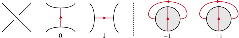
![[Uncaptioned image]](/html/0909.0816/assets/x2.png)
![[Uncaptioned image]](/html/0909.0816/assets/x3.png)