Computation of Spatial Skyline Points

Abstract

We discuss a method of finding skyline or non-dominated sites in a set $P$ of $n$ point sites with respect to a set $S$ of $m$ points. A site $p\in P$ is non-dominated if and only if for each $q\in P\setminus\{p\}$, there exists at least one point $s\in S$ that is closer to $p$ than to $q$. We reduce this problem of determining non-dominated sites to the problem of finding sites that have non-empty cells in an additively weighted Voronoi diagram under a convex distance function. The weights of said Voronoi diagram are derived from the coordinates of the sites of $P$, while the convex distance function is derived from $S$. In the two-dimensional plane, this reduction gives an $O((n+m)\log(n+m))$-time algorithm to find the non-dominated points.

1 Introduction

Consider a hotel recommendation system for a city with many hotels, located at point sites $P=\{p_{1},\ldots,p_{n}\}$. A tourist proposes to visit a set of $m$ locations of interest, $S=\{$museum $s_{1}$, restaurant $s_{2}$, garden $s_{3}$, …, beach $s_{m}\}$, and would like a short list of hotels near these locations. The system need not list any hotel $p\in P$ that is farther from all locations in $S$ than some other hotel $q\in P$.

It turns out that this is a special case of a problem considered in the database community [3, 17]. Consider a database whose entries are objects with $d$ attributes of interest. Given two objects $p$ and $q$, we write $p\succcurlyeq q$ if every attribute of $p$ is larger or equal to the corresponding attribute of $q$. If $p\succcurlyeq q$ but not $q\succcurlyeq p$, then we say that $p$ dominates $q$. An object is called non-dominated or a skyline object if it is not dominated by any object in the database. A skyline query is the problem of determining the skyline objects in a database with respect to a given set of attributes. Börzsönyi et al. [3] proposed to add a skyline operator to solve skyline queries in an existing (relational, object-oriented, or object-relational) database system.

Our hotel recommendation problem fits this framework exactly if we choose the attributes of each point in $P$ to be the negative distances to the points in $S$. Sharifzadeh and Shahabi [17] use the term spatial skyline query for this special version of the problem. They suggest other application scenarios in defense or crisis management, such as identifying a set of buildings that are to be evacuated ahead of other buildings in case of multiple fires.

In a spatial skyline query, the distances to the points of $S$ are considered attributes describing the sites of $P$. A site $p\in P$ dominates $q\in P$ if and only if it is strictly better in at least one attribute and is at least as good in all attributes. In our scenario for a hotel recommendation system, if $p\in P$ is dominated by $q\in P$, then $p$ need not be on the short list of hotels for a tourist visiting $S$. On the other hand, if $p\in P$ is not dominated by any $q\in P$, then $p$ is a non-dominated point site or a skyline point. Examples of skyline points are the discrete Fermat-Weber point, which is the site in $P$ that minimizes the sum of distances to the points $S$, and the sites in $P$ that are a nearest neighbor of some point in $S$.

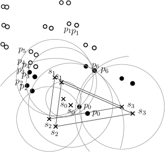
Figure 1: Among the hotels at sites $P$ (small circles), the five filled circles are the skyline points for the locations $S=\{s_{0},\ldots,s_{3}\}$ (crosses). Four larger circles with centers in $S$, passing through $p_{0}$, show that most sites are dominated by $p_{0}$. Sites $p_{4}$ and $p_{5}$ are not, but are dominated by $p_{3}$.

We will use the Euclidean metric, although other metrics can be substituted, often without changing the set of skyline points. Since the distance from each point $s\in S$ becomes an attribute of an object, and objects are compared only attribute-wise, any metric that increases monotonically with increasing Euclidean distance will identify the same set of skyline points. In fact, after retrieving the short list of hotels, our tourist could even use a separate metric $d_{s}$ for the distance to each site $s\in S$ to reflect his or her interest in each site. Because they are defined by dominance, our tourist is guaranteed not only that the best hotel is present on the short list, but also that every hotel on the list is the best for some combination of the distances. More formally, the skyline points are exactly the sites $p\in P$ that minimize the sum $f(p)=\sum_{s\in S}d_{s}(p,s)$ for some choice of weighted distance functions $d_{s}$ [3]. Thus, they generalize the discrete Fermat-Weber points.

Prior Work.

The skyline problem and its variants were named by researchers in the database community [3, 17]. Börzsönyi et al. [3] gave details for implementing a divide and conquer algorithm from computational geometry [10, 14] in a database context to take $O(n\log^{d-2}n+dn\log n)$ time for $d$ attributes of interest. Since then, several other works have used nearest neighbor search [9], sorting [5] and index structures [13, 22], primarily aiming to show an experimental improvement over the results of Börzsönyi et al. [3].

To apply the method of Börzsönyi et al. to a spatial skyline query with $n$ candidate sites and $m$ locations of interest determining the attributes, one would build the attribute vectors and then compute the skyline points in $O(n\log^{m-2}n+mn\log n)$ time.

For the planar case, Sharifzadeh et al. [18], correcting an error in their earlier algorithm [17] that was pointed out by Son et al. [20], give two algorithms for the problem, one based on R-trees, one based on a transversal of Voronoi diagrams and Delaunay triangulations, and compare them experimentally.

Lee et al. [11] give an algorithm that runs in time $O(n(s\log m+n))$, where $s$ is the number of reported skyline points. In the worst case, this is $O(n^{2}\log m)$. They show that both the worst-case running time and the experimental performance of their algorithm is significantly better than the algorithms by Sharifzadeh et al. [18]. They also give an approximation algorithm.

Since it appears hard to improve beyond quadratic running time under the Euclidean metric, Son et al. [19] consider skyline points under the Manhattan metric instead, and are able to give an $O((n+m)\log(n+m))$-time algorithm.

Another line of research suggests that in situations where there are many skyline points, the user may be better served by reporting only the top $k$ skyline points, with respect to some scoring function. Goncalves and Vidal [7] give an algorithm that solves this problem in $O(n^{2}d)$ time, where $d$ is the number of attributes defining the skyline points. Returning to the spatial setting, Son et al. [21] consider the problem of reporting the top-$k$ skyline points under the Manhattan metric, achieving an $O(\log n)$ improvement compared to computing all skyline points and ranking those.

Results.

We first discuss the formal definition and some degenerate situations in Section 2. In Section 3 we then use lifting techniques [4] to give several geometric views of dominance and non-dominance problems, involving balls, lower envelopes of cones, and Voronoi diagrams with a convex polygonal distance function (determined by $S$) and additive weights (determined by $P$).

In Section 4 we turn to the situation where the sites $P$ and points $S$ are given in the two-dimensional plane. Here we can turn our transformations into an efficient algorithm with running time $O((n+m)\log(n+m))$ . This is the first algorithm to improve upon the quadratic time barrier, and matches the bound for the Manhattan distance by Son et al. [19].

After the transformation, our algorithm solves the following question: given a convex polygonal cone $\mathcal{C}$ of complexity $m$ in $\mathbb{R}^{3}$, and $n$ translation vectors $t_{1},\dots,t_{n}$, decide which of the translated cones $\mathcal{C}+t_{i}$ are redundant in the sense that they do not contribute to the union of the $n$ cones. Since the union of the cones is equivalent to their lower envelope, a cone $\mathcal{C}+t_{i}$ is redundant exactly if its apex does not appear on the lower envelope of the family of cones.

We make use of a recent algorithm by Biniaz et al. [2], who transform a different problem (on the existence of a two-point consistent subset) to a similar question about translates of a convex polygonal cone. The key idea is to represent the union of the cones using the compact representation of Voronoi diagrams by McAllister et al. [12]—while the complexity of the union could be $\Theta(nm)$, the compact representation has complexity $O(n)$—and to use a simplified version of their sweep-line algorithm for the computation of Voronoi diagrams to answer our question.

2 Preliminaries

Throughout the paper, $P$ will denote a set of $n$ point sites, and $S$ will denote a set of $m$ points (locations) in $\mathbb{R}^{d}$. We use $d(x,y)$ for the usual $L_{2}$-distance in $\mathbb{R}^{d}$. For a set $X\subset\mathbb{R}^{d}$, we denote its interior as $\operatorname{int}X$.

For two sites $p,q\in P$ we write $p\succcurlyeq q$ if $d(p,s)\leqslant d(q,s)$ for every $s\in S$. A site $p\in P$ dominates $q\in P$ if $p\succcurlyeq q$ but not $q\succcurlyeq p$, which is equivalent to saying that we have $d(p,s)\leqslant d(q,s)$ for all $s\in S$ and $d(p,s)<d(q,s)$ for at least one $s\in S$. If $p\in P$ is not dominated by any $q\in P$, then $p$ is a non-dominated point site or a skyline point.

Let us first investigate the case of two sites $p,q\in P$ with $p\succcurlyeq q$ and $q\succcurlyeq p$. This implies that $d(p,s)=d(q,s)$ for all points in $S$. In other words, all points in $S$ lie on the bisector of $p$ and $q$, and therefore in a flat of dimension at most $d-1$. We can ensure that this case does not arise by a simple preprocessing of the point set: Let $H$ be the affine hull of $S$. If $H$ has dimension $k<d$, then we replace $P$ by a point set in $k+1$ dimensions that preserves all distances to the flat $H$ and such that $P$ is contained in one closed halfspace of $\mathbb{R}^{k+1}$ bounded by $H$. With this preprocessing, we will have that for any two sites $p\neq q$ in $P$, we always have $d(p,s)\neq d(q,s)$ for some $s\in S$, and we will make this assumption throughout the paper. Note that the preprocessing may map several sites of $P$ into the same point—either all the original sites are skyline points, or none of them is.

With this assumption, $p\in P$ dominates $q\in P\setminus\{p\}$ simply if $p\succcurlyeq q$, that is if $d(p,s)\leqslant d(q,s)$ for all $s\in S$. Conversely, $p$ is not dominated by $q$ if and only if there is a site $s\in S$ such that $d(p,s)<d(q,s)$. It follows that a site $p\in P$ is a skyline point if and only if for every site $q\in P\setminus\{p\}$ there is a site $s_{q}\in S$ with $d(p,s_{q})<d(q,s_{q})$.

Our problem is to extract the skyline points of $P$ with respect to $S$. Let $h(p,q)$ denote the half-plane containing $p$ that is bounded by the bisector of $p$ and $q$. A brute force approach to identify whether $p\in P$ is a skyline point is to determine, for all $q\neq p$, if at least one site $s\in S$ lies in $h(p,q)$. This takes $\Theta(mn)$ time for each $p$, giving a total time of $\Theta(mn^{2})$.

3 Views of non-dominance problems in $\mathbb{R}^{d}$

We first relate point domination in $d$ dimensions to balls (disks as in Figure 1), then to the envelope of cones, and finally to the additively weighted Voronoi diagram of a convex distance function. We will define these terms as we go, culminating in the following Theorem 4, which we prove at the end of the section.

Theorem 4.

The skyline or non-dominated points of a set $P\subset\mathbb{R}^{d}$ with respect to locations $S\subset\mathbb{R}^{d}$ are those with non-empty Voronoi cells under a convex distance function determined by $S$ with additive weights determined by $P$.

In Section 4, we will show that for sites and locations in the plane, the reduction implied by Theorem 4 leads to an efficient algorithm.

3.1 Dominated points and balls

For $x,y\in\mathbb{R}^{d}$, let $C(x,y)$ denote the closed ball with center $x$ and radius $d(x,y)$. For a site $p\in P$, consider the balls $C(s,p)$ centered at each $s\in S$. Figure 1 illustrates that the sites dominated by $p_{0}$ are outside the union of the disks through $p_{0}$, that is, outside $\bigcup_{s\in S}C(s,p_{0})$. On the other hand, Figure 2 illustrates that $p_{6}$ is not dominated, because no site of $P$ is inside the intersection of its disks. These two complementary views of dominance and non-dominance can be contrasted throughout the entire Section 3.

Figure 2: Site $p_{6}$ is not dominated.

For $p\in P$, we define the dominator region of $p$ as $D_{p}=\bigcap_{s\in S}C(s,p)$, and the dominated region of $p$ as $\mathcal{D}_{p}=\mathbb{R}^{d}\setminus\bigcup_{s\in S}\operatorname{int}C(s,p)=\bigcap_{s\in S}\big{(}\mathbb{R}^{d}\setminus\operatorname{int}C(s,p)\big{)}$. We make the following observations:

Observation 1.

For site $p\in P$ we have:

(i)

a site $q\in P$ dominates $p$ if and only if $q\in D_{p}$;

(ii)

$p$ dominates a site $q\in P$ if and only if $q\in\mathcal{D}_{p}$;

(iii)

$p$ is a skyline point if and only if $D_{p}$ does not contain any site $q\in P\setminus\{p\}$;

(iv)

$p$ is a skyline point if and only if $p\not\in\mathcal{D}_{q}$ for all $q\in P\setminus\{p\}$;

(v)

if a site $q\in P$ lies in $D_{p}$ then $D_{q}\subset D_{p}$;

(vi)

if a site $q\in P$ lies in $\mathcal{D}_{p}$, then $\mathcal{D}_{q}\subset\mathcal{D}_{p}$;

(vii)

$D_{p}$ is a non-empty convex region bounded by spherical patches centered at vertices of the convex hull of sites, ${\cal CH}(S)$.

Proof.

We have $q\succcurlyeq p$ if and only if $d(q,s)\leqslant d(p,s)$ for all $s\in S$, which is equivalent to $q\in C(s,p)$ for all $s\in S$, or $q\in D_{p}$, implying claim (i).

On the other hand $p\succcurlyeq q$ if $d(p,s)\leqslant d(q,s)$ for all $s\in S$. This is equivalent to $q\not\in\operatorname{int}C(s,p)$ for all $s\in S$, or $q\not\in\bigcup_{s\in S}\operatorname{int}C(s,p)$, implying claim (ii).

Claims (iii) and (iv) now follow immediately from the definition of skyline points.

For (v), $q\in D_{p}$ implies $q\succcurlyeq p$, or $d(q,s)\leqslant d(p,s)$ for all $s\in S$. Then $C(s,q)\subseteq C(s,p)$ for all $s\in S$, and so $D_{q}\subset D_{p}$.

For (vi), $q\in\mathcal{D}_{p}$ implies $p\succcurlyeq q$, or $d(p,s)\leqslant d(q,s)$ for all $s\in S$. Then $\operatorname{int}C(s,p)\subseteq\operatorname{int}C(s,q)$, and $\bigcup_{s\in S}\operatorname{int}C(s,p)\subset\bigcup_{s\in S}\operatorname{int}C(s,q)$. This implies $\mathcal{D}_{p}\supset\mathcal{D}_{q}$.

For (vii) we observe that $D_{p}$ is the intersection of balls and therefore convex and bounded by spherical patches; since all balls contain $p$, the intersection is not empty. Fix a unit vector $v$ and consider where the ray from $p$ in direction $v$ leaves $D_{p}$: $\max_{\alpha}(p+\alpha v)\in D_{p}$. For each inequality $d(p+\alpha v,s)\leqslant d(p,s)$, we can square both sides and rewrite as $\alpha\leqslant 2(s-p)\cdot v$. Thus, $\alpha$ is determined by the extreme site $s$ in direction $v$, and this site is on the convex hull, $\mathcal{CH}(S)$. ∎

In the plane, the boundary of the dominator region $D_{p}$ is determined by at most $m$ circular arcs, and so the total complexity of the dominator regions for all the sites in $P$ is $\Theta(mn)$.

Since the dominated region is non-convex, it looks more complex to work with, but in fact this distinction will disappear as we lift to cones in the next subsection.

3.2 Dominator cones and dominated cones

We use Brown’s lifting map to generate cones from balls [4]. Assume a coordinate system with origin inside the convex hull $\mathcal{CH}(S)$. Consider sites and locations in the plane for the moment, and lift $S$ and $P$ to the unit paraboloid $\Psi=\{(x,y,z)\mid z=x^{2}+y^{2}\}$; a point $p=(x,y)$ in the plane is lifted to the point $p^{\prime}=(x,y,x^{2}+y^{2})$ on $\Psi$. Note that lifting a circle $C=\{(x-c_{1})^{2}+(y-c_{2})^{2}=r^{2}\}$ gives a set $C^{\prime}=\{z-2c_{1}x-2c_{2}y+c_{1}^{2}+c_{2}^{2}-r^{2}=0\}$ on $\Psi$ that is linear in $x$, $y$, and $z$ [15]. Thus, we can consider $C^{\prime}$ to be a plane in $3$-dimensional space. Points inside the circle $C$ are lifted to points on the paraboloid $\Psi$ that lie in the halfspace below $C^{\prime}$, which we denote $C^{-}$. Points outside the circle map to points on $\Psi$ that lie in the halfspace above, denoted $C^{+}$.

Lifting in higher dimensions is analogous, with $p^{\prime}$ adding a final dimension of $p\cdot p$ to a point $p\in\mathbb{R}^{d}$, and spheres being lifted to hyperplanes. For a ball $C(s,p)$, we denote the lifted hyperplane as $C^{\prime}(s,p)$, the closed halfspace below this hyperplane as $C^{-}(s,p)$, and the closed halfspace above the hyperplane as $C^{+}(s,p)$.

For $p\in P$, we define the dominator cone $\Lambda_{p}=\bigcap_{s\in S}C^{-}(s,p)$, and the dominated cone $V_{p}=\bigcap_{s\in S}C^{+}(s,p)$. They are directly related to the dominator region and dominated region as follows:

Observation 2.

For points $q\in\mathbb{R}^{d}$ and $p\in P$, we have $q\in D_{p}$ if and only if $q^{\prime}\in\Lambda_{p}$, and $q\in\mathcal{D}_{p}$ if and only if $q^{\prime}\in V_{p}$.

Proof.

We have $q\in C(s,p)$ if and only if $q^{\prime}\in C^{-}(s,p)$. It follows that $q\in D_{p}=\bigcap_{s\in S}C(s,p)$ if and only if $q^{\prime}\in\bigcap_{s\in S}\Lambda_{p}=C^{-}(s,p)$. Similarly $q\not\in\operatorname{int}C(s,p)$ if and only if $q^{\prime}\in C^{+}(s,p)$. It follows that $q\in\mathcal{D}_{p}=\bigcap_{s\in S}\big{(}\mathbb{R}^{d}\setminus\operatorname{int}C(s,p)\big{)}$ if and only if $q^{\prime}\in V_{p}=\bigcap_{s\in S}C^{+}(s,p)$. ∎

Let $o$ denote the origin of the coordinate system, so that $o^{\prime}=o$, and consider the cones $\Lambda=\bigcap_{s\in S}C^{-}(s,o)$ and $V=\bigcap_{s\in S}C^{+}(s,o)$. Since $C^{\prime}(s,o)$ passes through $o$, both cones have their apex in $o$, and since $C^{+}(s,o)=-C^{-}(s,o)$, we have $V=-\Lambda$.

Now we observe that the hyperplane $C^{\prime}(s,p)$ is parallel to the hyperplane tangent to the unit paraboloid in $s^{\prime}$, and passes through $p^{\prime}$. It follows that $C^{\prime}(s,p)=C^{\prime}(s,o)+p^{\prime}$, and so $\Lambda_{p}=\Lambda+p^{\prime}$ and $V_{p}=V+p^{\prime}$. In particular, all dominator cones are translates of $\Lambda$—and all dominated cones are translates of $V$. Both $\Lambda_{p}$ and $V_{p}$ have their apex in $p^{\prime}$.

Consider two points $p,q\in P$. By Observations 1(i) and 2, $q$ dominates $p$ if and only if $q^{\prime}\in\Lambda_{p}$. Since $\Lambda_{p}$ and $\Lambda_{q}$ are homothets, this is equivalent to $\Lambda_{q}\subset\Lambda_{p}$. By the same reasoning, $q$ dominates $p$ if and only if $V_{p}\subset V_{q}$. (Note that these properties imply Observations 1(v)–(vi).)

The union of a set of upward-pointing cones is known as its lower envelope; Figure 3(right) shows an example. We say that cone $V_{p}$ is redundant if the union of the cones $V_{q}$, for $q\in P\setminus\{p\}$, already contains $V_{p}$.

Corollary 3.

The skyline points among the sites $P$ with respect to the points $S$ correspond exactly to the non-redundant cones in the lower envelope.

Proof.

Since all cones are homothets, a cone $V_{p}$ is redundant if and only if $p^{\prime}\in V_{q}$, for some $q\in P\setminus\{p\}$. We have $p^{\prime}\in V_{q}$ if and only if $q$ dominates $p$, so the claim follows. ∎

3.3 Additively weighted Voronoi diagrams under a convex distance function

Constructing the lower envelope of the cones $V_{p}$ is costly; the best algorithm known would take $\Theta(nm\log(m+n))$ time even in dimension two. However, lower envelopes of cones can be interpreted as Voronoi-diagrams, and this will lead us to a more efficient method of finding the non-redundant cones.

Minkowski showed that any compact convex set $M$ whose interior contains the origin defines a convex distance function $d_{M}(p,q)$, where the distance from point $p$ to $q$ with respect to $M$ is the amount that $M$ must be scaled to include $q-p$. Mathematically,

$$d_{M}(p,q)=\min\{\lambda\geqslant 0\mid q-p\in\lambda M\}$$

A convex distance function may not be a metric, since $d_{M}$ is symmetric only if $M$ is centrally symmetric: we have $d_{M}(p,q)=d_{-M}(q,p)$. However, the distance function $d_{M}$ satisfies the triangle inequality [16]: $d_{M}(p,q)+d_{M}(q,r)\geqslant d_{M}(p,r).$ The boundary of $M$ serves as the unit ball for the distance function $d_{M}$. For a fixed $p$, the graph of $x\mapsto d_{M}(p,x)$ is a cone with apex at $p$, and every horizontal cross-section is a homothet of $M$. Note that the Euclidean metric is the convex distance function with $M$ the unit-radius ball.

Given a finite set of points $P\subset\mathbb{R}^{d}$ with additive weights $\omega_{p}$ for each $p\in P$, and a convex distance function $d_{M}(p,q)$, we define the Voronoi cell of a point $p\in P$ as

$$\mathcal{V}(p)=\Big{\{}x\in\mathbb{R}^{d}\Bigm{|}d_{M}(p,x)+\omega_{P}<d_{M}(q,x)+\omega_{q}\text{~{}for all~{}}q\in P\setminus\{p\}\Big{\}}.$$

The Voronoi diagram of $P$ is the family of all Voronoi cells $V(p)$, for $p\in P$.

Figure 3(left) shows the Voronoi diagram of six distinct sites in the plane, all having weight zero. The distance function is defined by the black convex quadrilateral around the point at the origin, and each Voronoi cell is drawn in a different shade.

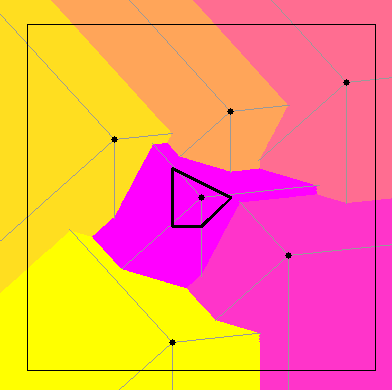
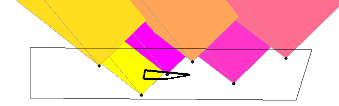
Figure 3: A Voronoi diagram of 6 sites in the plane using a convex quadrilateral as distance function; its view as a lower envelope of cones. All weights are zero to make the 3d figure easier to interpret.

Every Voronoi diagram is the minimization diagram of a family of functions. We define $f_{p}(x)=d_{M}(p,x)+\omega_{p}$ for $p\in P$, and consider the lower envelope of these functions, that is, the graph of the function $f_{\min}:x\mapsto\min_{p\in P}f_{p}(x)$. The Voronoi cell of $p$ is the set of all those $x$ where $f_{p}(x)=f_{\min}(x)$ and $f_{q}(x)>f_{\min}(x)$ for $q\neq p$. In this sense, the Voronoi diagram corresponds to the projection of the graph of $f_{\min}$. Since the graph of each $f_{p}$ is a cone with apex at $(p,\omega_{p})$, the Voronoi diagram corresponds to the lower envelope of these cones, see Figure 3(right) for an illustration.

Theorem 4.

The skyline or non-dominated points among the sites $P$ with respect to points $S$ are those with non-empty Voronoi cells under a convex distance function determined by $S$ with additive weights determined by $P$.

Proof.

Consider the $(d+1)$-dimensional cone $V=\bigcap_{s\in S}C^{+}(s,o)$. The intersection of this cone with the plane $x_{d+1}=1$ is a $d$-dimensional convex polytope $M$ that contains the point $(0,0,\dots,0,1)$. The boundary of $V$ is therefore the graph of the function $x\mapsto d_{M}(o,x)$. Since for $p\in P$, we have $V_{p}=V+p^{\prime}$, the boundary of $V_{p}$ is the graph of $x\mapsto f_{p}(x)=d_{M}(p,x)+\omega_{p}$, where $\omega_{p}=p\cdot p$.

It follows that the lower envelope of the cones $V_{p}$ corresponds to the Voronoi diagram of $P$ with additive weights $\omega_{p}=p\cdot p$ and convex distance function $d_{M}$, where $M$ is defined entirely by the points $S$.

A point $p\in P$ is a skyline point if $V_{p}$ is not redundant, which is equivalent to $p^{\prime}$ not lying in any cone $V_{q}$, for $q\in P\setminus\{p\}$. If this is the case, then $f_{p}(p)<f_{q}(p)$ for $q\in P\setminus\{p\}$, and so the Voronoi cell of $p$ contains at least $p$ itself and is not empty. If $p^{\prime}\in V_{q}$ for some $q\neq p$, then we have $V_{p}\subset V_{q}$. This implies $f_{p}(x)\geqslant f_{q}(x)$ for all $x$, and so the Voronoi cell of $p$ is empty. ∎

4 Computing the non-redundant cones

We now focus on sites and locations in the plane, because in this important case the reductions of the previous section can be turned into an efficient algorithm.

By Theorem 4, it would suffice to compute a Voronoi diagram and check which sites define non-empty Voronoi cells. Unfortunately, to our knowledge, Voronoi diagrams under convex distance functions with additive weights have not been studied in the literature [6].

Fortunately, Biniaz et al. [2] recently showed how to solve a specific problem about such diagrams: Given $n$ sites with additive weights, a convex distance function defined by a convex $n$-gon, and $n$ query points, they determine the Voronoi cell containing each query point. They use a simplified version of the sweepline algorithm by McAllister et al. [12] to solve this problem without actually computing the Voronoi diagram. As they already point out, their algorithm can easily be adapted to solve our problem of determining the non-empty Voronoi cells. In the following we sketch their algorithm as applied to our problem, referring the reader to Biniaz et al. [2] and McAllister et al. [12] for details.

We start by picking a coordinate system such that no two sites have the same $x$-coordinate. We then process the points $S$ in $O(m\log m)$ time to compute the cone $V=\bigcap_{s\in S}C^{+}(s,o)$. A horizontal cross section of $V$ is a convex polygon whose edges correspond to the extreme points in $S$, so it has at most $m$ edges.

By Theorem 4, our goal is to determine which elements of the family of cones $\{V+p^{\prime}\mid p\in P\}$ are non-redundant in the lower envelope of the family. We split the cone $V$ along the $yz$-plane, resulting in a cone $V^{\prime}$ in the half-space $x\geqslant 0$, and a cone $V^{\prime\prime}$ in the half-space $x\leqslant 0$. We define $V_{p}=V+p^{\prime}$, $V^{\prime}_{p}=V^{\prime}+p^{\prime}$, and $V^{\prime\prime}_{p}=V^{\prime\prime}+p^{\prime}$. Since $V_{p}\subset V_{q}$ is equivalent to $p^{\prime}\in V_{q}=V^{\prime}_{q}\cup V^{\prime\prime}_{q}$, $V_{p}$ is redundant if and only if $V^{\prime}_{p}$ is redundant in the family $\{V^{\prime}_{p}\mid p\in P\}$ or $V^{\prime\prime}_{p}$ is redundant in the family $\{V^{\prime\prime}_{p}\mid p\in P\}$.

We explain how to determine the non-redundant cones in the lower envelope of the family $\{V^{\prime}_{p}\mid p\in P\}$. The treatment of the family $\{V^{\prime\prime}_{p}\mid p\in P\}$ is symmetrical. To make the lower envelope well-behaved, we remove all degeneracies by perturbing the additive weights $\omega_{p}$ slightly. To this end, we define the rank $\eta(p)$ of $p\in P$ as the number of points $q\in P$ with $q_{x}\leqslant p_{x}$. We have $1\leqslant\eta(p)\leqslant n$, and since no two points have the same $x$-coordinate, all ranks are distinct. We perturb $\omega_{p}$ to $\omega_{p}-\varepsilon^{\eta(p)}$, for an infinitesimal $\varepsilon>0$. With this perturbation, we achieve that (i) no apex of a cone lies on the boundary of another cone, (ii) any three cone boundaries have a finite number of points in common, and (iii) no four cone boundaries have a point in common. Consider now a pair of cones with $V^{\prime}_{p}\subset V^{\prime}_{q}$. This is equivalent to $p^{\prime}\in V^{\prime}_{q}$, which implies that $\eta(p)>\eta(q)$. We therefore have $\varepsilon^{\eta(p)}\ll\varepsilon^{\eta(q)}$, and so the perturbation preserves the containment. It follows that the set of non-redundant cones remains unchanged by the perturbation.

As before, we interpret the boundary of the cone $V^{\prime}_{p}$ as the graph of a function $f_{p}$. The function $f_{p}$ is now a partial function, defined only on the half-plane $x\geqslant p_{x}$. We define $f_{\min}(x,y)=\min_{p\in P,p_{x}\leqslant x}f_{p}(x,y)$, and the regions $\mathcal{R}_{p}$ where $f_{p}$ gives the minimum:

$$\mathcal{R}_{p}=\bigl{\{}(x,y)\bigm{|}f_{p}(x,y)=f_{\min}(x,y)\bigr{\}}.$$

Because of our perturbation, the regions $\mathcal{R}_{p}$ are interior-disjoint, and their closures cover the half-plane bounded by the vertical line through the leftmost site. A cone $V^{\prime}_{p}$ is redundant if and only if $\mathcal{R}_{p}$ is empty. Biniaz et al. [2] observe the following folklore properties of the regions $\mathcal{R}_{p}$:

• $\mathcal{R}_{p}$ is star-shaped with respect to $p$: For every $x\in\mathcal{R}_{p}$, the segment $px$ lies in $\mathcal{R}_{p}$.

• For three distinct sites $p,q,r\in P$, the intersection $\mathcal{R}_{p}\cap\mathcal{R}_{q}\cap\mathcal{R}_{r}$ contains at most two points.

We add the following observation:

Lemma 5.

For two distinct sites $p,q\in P$ the intersection $\mathcal{R}_{p}\cap\mathcal{R}_{q}$ is $x$-monotone in each half-plane bounded by the line $pq$.

Proof.

We can assume $\eta(p)<\eta(q)$ and consider the half-plane above the line $pq$. Assume there are two points $s_{1}=(x,y_{1})$ and $s_{2}=(x,y_{2})$, with $y_{1}<y_{2}$, that lie in $\mathcal{R}_{p}\cap\mathcal{R}_{q}$. Then the segment $ps_{1}$ lying in $\mathcal{R}_{p}$ and the segment $qs_{2}$ lying in $\mathcal{R}_{q}$ intersect, a contradiction. ∎

Biniaz et al. [2] show how to adapt [12, Lemma 3.15], which makes use of Kirkpatrick and Snoeyink’s tentative prune-and-search technique [8], to perform each of the following computations in $O(\log m)$ time:

• Given a point $(x,y)$ and $p\in P$, evaluate $f_{p}(x,y)$;

• Given three distinct sites $p,q,r\in P$, compute $\mathcal{R}_{p}\cap\mathcal{R}_{q}\cap\mathcal{R}_{r}$;

• Given two distinct sites $p,q\in P$ and a vertical line $\ell$, compute $\ell\cap\mathcal{R}_{p}\cap\mathcal{R}_{q}$.

Armed with these primitives, we can now explain the algorithm. We sweep a vertical line $\ell\equiv\bigl{\{}(x,y)\bigm{|}x=t\bigr{\}}$, where $t$ goes from $-\infty$ to $+\infty$. During the sweep, we maintain the sequence of regions $\mathcal{R}_{p}$ intersected by the sweepline, in order of increasing $y$-coordinate. A fixed region $\mathcal{R}_{p}$ may appear several times in this sequence. For each element of the sequence except the topmost and bottommost one, we maintain a spoke: a non-vertical line segment or half-line intersecting the sweepline inside the region. More precisely, when $\mathcal{R}_{p}$ appears on the sweepline with upper neighbor $\mathcal{R}_{q}$ and lower neighbor $\mathcal{R}_{r}$, then the spoke connects $p$ with the “vertex” $v=\mathcal{R}_{q}\cap\mathcal{R}_{p}\cap\mathcal{R}_{r}$ where $q,p,r$ appear counter-clockwise in this order around $v$. If no such point $v$ exists, then the spoke extends up to infinity.

When there are $k$ elements in the sweepline sequence, we thus have $k-2$ spokes that separate the sweepline into $k-1$ intervals. Each interval belongs to two adjacent regions.

Since the bisectors $\mathcal{R}_{p}\cap\mathcal{R}_{q}$ are $x$-monotone, the sequence of regions intersecting the sweepline changes in only two ways: At a site event, the sweep line reaches one of the sites $P$, which can cause a new region to appear. At a vertex event, we reach (locally) the end of a region. The point where this happens is necessarily the endpoint of the spoke for the region.

The sweep is initialized by adding the first three sites to the sweepline status. In $O(\log m)$ time we determine the order of the regions along the sweepline and compute the spoke for the middle element. We add the spoke endpoint as a vertex event to the event queue.

At a vertex event, we first check if the regions $\mathcal{R}_{p},\mathcal{R}_{q},\mathcal{R}_{r}$ defining the spoke endpoint are still adjacent on the sweepline. If not, we can ignore the event. Otherwise, we remove $\mathcal{R}_{q}$ from the sweepline status. This causes the lower neighbor of $\mathcal{R}_{p}$ and the upper neighbor of $\mathcal{R}_{r}$ to change, so we recompute their spokes and add the new spoke endpoints to the event queue. All this takes $O(\log n+\log m)$ time.

Consider now a site event, where the sweepline reaches site $p\in P$. We perform binary search on the spokes to locate the interval between two spoke segments containing $p$. Since the spoke segments are given geometrically, this takes $O(\log n)$ time. Once we know that $p$ lies in one of the two regions $\mathcal{R}_{q}$ or $\mathcal{R}_{r}$, we evaluate $f_{q}(p)$ and $f_{r}(p)$. Let’s say that $f_{q}(p)<f_{r}(p)$, so that $p$ lies in $\mathcal{R}_{q}$. If $f_{q}(p)<\omega_{p}$, then $\mathcal{R}_{p}$ is empty and $V^{\prime}_{p}$ is redundant, and we are done with the site. Otherwise, $V^{\prime}_{p}$ is not redundant, and $\mathcal{R}_{p}$ needs to be inserted into the sweepline status. We duplicate the region for $\mathcal{R}_{q}$ and insert $\mathcal{R}_{p}$ between the two copies. We then walk up and down the sweepline status from $p$ to determine whether and which regions disappear from the sweepline status. We can decide that for a region $\mathcal{R}_{s}$ by computing its intersection with the sweepline in $O(\log m)$ time, and evaluating $f_{s}$ and $f_{p}$ at those points. Finally, we compute the spoke segment for $\mathcal{R}_{p}$ and recompute it for the two neighbors of $\mathcal{R}_{p}$ in the sweepline status, inserting the spoke endpoints into the event queue. Handling the event thus takes time $O(\log n+(k+1)\log m)$, where $k$ is the number of regions removed from the sweepline status.

A site event increases the size of the sweepline status by at most two, and creates at most three vertex events. A vertex event creates up to two new vertex events, but only if it removes a region from the sweepline status. We can thus charge the vertex events to the at most $2n$ regions ever appearing on the sweepline status, and observe that both sweepline status and event queue have size $O(n)$. The total running time is thus $O\bigl{(}m\log m+n(\log n+\log m)\bigr{)}=O\bigl{(}(n+m)\log(n+m)\bigr{)}$.

We summarize this section with the following theorem.

Theorem 6.

The skyline or non-dominated points among $n$ sites in the plane with respect to a set of $m$ locations can be computed in time $O\bigl{(}(n+m)\log(n+m)\bigr{)}$.

5 Conclusions

In this paper, we proposed an algorithm for finding the non-dominated or skyline points among a point set $P$ with respect to a set of sites $S$ in $\mathbb{R}^{2}$. This problem was initially proposed by Sharifzadeh and Shahabi [17] and termed the spatial skyline query problem. We gave some geometric insights into this problem to design an efficient algorithm to find the skyline points, especially when the points and sites are given in the plane.

Since our reductions apply in all dimensions, it would be interesting to extend the algorithms to dimensions higher than two, although for geographical applications, the 2-d map is the most relevant. It may be more important to consider dynamic versions of spatial skyline queries that support insertion and deletion of sites and data points, and to combine 2-d spatial skyline queries with one or more non-spatial attributes. The decomposability of skyline queries means that there are interesting trade-offs to be considered when partitioning the problem on spatial or non-spatial dimensions.

References

- [1] B. K. Bhattacharya, A. Bishnu, O. Cheong, S. Das, A. Karmakar, and J. Snoeyink. Computation of non-dominated points using compact Voronoi diagrams. In WALCOM: Algorithms and Computation, pages 82–93, 2010.
- [2] A. Biniaz, S. Cabello, A. Maheshwari, P. Carmi, S. Mehrabi, J. D. Carufel, and M. H. M. Smid. On the minimum consistent subset problem. CoRR, abs/1810.09232, 2018.
- [3] S. Börzsönyi, D. Kossmann, and K. Stocker. The skyline operator. In Proceedings of the 17th International Conference on Data Engineering, pages 421–430, Washington, DC, USA, 2001. IEEE Computer Society.
- [4] K. Q. Brown. Geometric transforms for fast geometric algorithms. Ph.D. thesis, Dept. Comput. Sci., Carnegie-Mellon Univ., Pittsburgh, PA, 1980. Report CMU-CS-80-101.
- [5] J. Chomicki, P. Godfrey, J. Gryz, and D. Liang. Skyline with presorting. In Proceedings of the 17th International Conference on Data Engineering, pages 717–816, Washington, DC, USA, 2003. IEEE Computer Society.
- [6] S. Fortune. Voronoi diagrams and Delaunay triangulations. In J. E. Goodman and J. O’Rourke, editors, Handbook of Discrete and Computational Geometry, chapter 23, pages 513–528. CRC Press LLC, Boca Raton, FL, 2004.
- [7] M. Goncalves and M. Vidal. Reaching the top of the skyline: An efficient indexed algorithm for top-k skyline queries. In 20th Int. Conf. Database and Expert Systems Applications (DEXA), pages 471–485, 2009.
- [8] D. Kirkpatrick and J. Snoeyink. Tentative prune-and-search for computing fixed-points with applications to geometric computation. Fundam. Inform., 22:353–370, 1995.
- [9] D. Kossmann, F. Ramsak, and S. Rost. Shooting stars in the sky: An online algorithm for skyline queries. In VLDB ’02: Proceedings of the 28th International Conference on Very Large Data Bases, pages 275–286, 2002.
- [10] H. T. Kung, F. Luccio, and F. P. Preparata. On finding the maxima of a set of vectors. J. ACM, 22:469–476, 1975.
- [11] M. Lee, W. Son, H. Ahn, and S. Hwang. Spatial skyline queries: exact and approximation algorithms. GeoInformatica, 15:665–697, 2011.
- [12] M. McAllister, D. Kirkpatrick, and J. Snoeyink. A compact piecewise-linear Voronoi diagram for convex sites in the plane. Discrete Comput. Geom., 15:73–105, 1996.
- [13] D. Papadias, Y. Tao, G. Fu, and B. Seeger. Progressive skyline computation in database systems. ACM Transaction on Database System, 30(1):41–82, 2005.
- [14] F. P. Preparata and M. I. Shamos. Computational Geometry: An Introduction. Springer-Verlag, New York, NY, 1985.
- [15] J.-R. Sack and J. Urrutia. Handbook of Computational Geometry. North-Holland, 2000.
- [16] R. Schneider. Convex Bodies: The Brunn–Minkowski Theory. Encyclopedia of Mathematics and its Applications. Cambridge University Press, 2014.
- [17] M. Sharifzadeh and C. Shahabi. The spatial skyline queries. In VLDB ’06: Proceedings of the 32nd International Conference on Very Large Data Bases, pages 751–762. VLDB Endowment, 2006.
- [18] M. Sharifzadeh, C. Shahabi, and L. Kazemi. Processing spatial skyline queries in both vector spaces and spatial network databases. ACM Trans. Database Syst., 34:14:1–14:45, 2009.
- [19] W. Son, S. Hwang, and H. Ahn. MSSQ: Manhattan spatial skyline queries. Inf. Syst., 40:67–83, 2014.
- [20] W. Son, M.-W. Lee, H.-K. Ahn, and S.-w. Hwang. Spatial skyline queries: An efficient geometric algorithm. In N. Mamoulis, T. Seidl, T. B. Pedersen, K. Torp, and I. Assent, editors, Advances in Spatial and Temporal Databases, pages 247–264. Springer, 2009.
- [21] W. Son, F. Stehn, C. Knauer, and H. Ahn. Top- Manhattan spatial skyline queries. Inf. Process. Lett., 123:27–35, 2017.
- [22] K.-L. Tan, P.-K. Eng, and B. C. Ooi. Efficient progressive skyline computation. In VLDB ’01: Proceedings of the 27th International Conference on Very Large Data Bases, pages 301–310, San Francisco, CA, USA, 2001. Morgan Kaufmann Publishers Inc.