Simulating and detecting artificial magnetic fields in trapped atoms

Abstract

A Bose-Einstein condensate exhibiting a nontrivial phase induces an artificial magnetic field in immersed impurity atoms trapped in a stationary, ring-shaped optical lattice. We present an effective Hamiltonian for the impurities for two condensate setups: the condensate in a rotating ring and in an excited rotational state in a stationary ring. We use Bogoliubov theory to derive analytical formulas for the induced artificial magnetic field and the hopping amplitude in the limit of low condensate temperature where the impurity dynamics is coherent. As methods for observing the artificial magnetic field we discuss time of flight imaging and mass current measurements. Moreover, we compare the analytical results of the effective model to numerical results of a corresponding two-species Bose-Hubbard model. We also study numerically the clustering properties of the impurities and the quantum chaotic behavior of the two-species Bose-Hubbard model.

I Introduction

A prominent application of ultracold atoms trapped in optical lattices is that of a quantum simulator of condensed matter models. The advantage of such a simulator is that the Hamiltonian defining the condensed matter model can be implemented almost perfectly, and the relevant parameters, such as interaction strength or lattice geometry, can be tuned in a wide parameter range Lewenstein et al. (2007); Jaksch and Zoller (2005). In contrast, for a given condensed matter system the Hamiltonian governing its dynamics is often difficult to find. Examples of effects which can be simulated with neutral atoms in optical lattice are the quantum Hall effect in two dimensions von Klitzing et al. (1980); Sørensen et al. (2005); Palmer and Jaksch (2006); Palmer et al. (2008) or persistent ground state currents in superconducting rings Schmidt (1997); Ryu et al. (2007).

Several interesting effects in condensed matter experiments typically require a system to be exposed to a magnetic field. Therefore, a quantum simulator of these effects needs to include or simulate such a magnetic field. Ultracold atoms offer several promising ways to achieve this goal. One idea is to rotate a gas of atoms close to the frequency of the harmonic confinement that traps the atoms. This may result in states also found in the quantum Hall effect Wilkin and Gunn (2000); Cooper et al. (2001); Schweikhard et al. (2004). However, the high rotation frequency $\Omega$ of the atoms introduces a large centrifugal term, which tends to destroy the atomic cloud. On the other hand, to reach the strongly correlated state the rotation frequency of the cloud and the frequency of the confining harmonic trap $\omega_{c}$ have to be balanced with high accuracy such that $1-Z/2N\tilde{a}_{s}\lesssim\Omega/\omega_{c}\lesssim 1-8\tilde{a}_{s}/ZN$, where $Z$ is the transverse distance over which the condensate is uniform, $N$ is the number of atoms, and $\tilde{a}_{s}$ is on the order of the s-wave scattering length Rosenbusch et al. (2002). The necessity of precise counterbalancing is alleviated, in principle, by using traps with potentials stronger than harmonic at the expense of harder experimental implementation Bretin et al. (2004). A different approach is to use lasers with an orbital angular momentum Juzeliūnas and Öhberg (2004); Juzeliūnas et al. (2005) or to use Raman-assisted hopping in a layered optical lattice geometry Jaksch and Zoller (2003) in order to mimic the effect of a magnetic field. Both proposals might also be difficult to realize experimentally.

In this paper, we analyze and extend methods introduced by some of the present authors Klein and Jaksch (2009) for simulating a magnetic field in atoms trapped in a ring-shaped, stationary optical lattice. These lattice atoms, in the following also called impurities, are immersed into a ring-shaped quasi-onedimensional Bose-Einstein condensate (BEC) exhibiting a nontrivial phase. For creating this phase we consider two possible setups. Firstly, a BEC trapped in a rotating ring Morizot et al. (2006); Gupta et al. (2005); Heathcote et al. (2008); secondly, a BEC carrying a quantized angular momentum in a stationary ring Nandi et al. (2004), i.e., a BEC in an excited state. In the former case, we can allow a confining potential to overcompensate the centrifugal term in the rotating BEC as we are mainly interested in the dynamics of the impurities. This is in contrast to methods for observing quantum Hall states directly in a rotating gas of ultracold atoms where the centrifugal term needs to be counterbalanced precisely Rosenbusch et al. (2002). The BEC is described in terms of Bogoliubov excitations, which couple to the impurity atoms. It has been shown in earlier publications that the presence of the phonon-impurity coupling leads to observable effects in the transport properties of the lattice atoms such as the transition from coherent to incoherent transport with increasing temperature or clustering Bruderer et al. (2007, 2008); Klein et al. (2007). In addition, by allowing the BEC to exhibit a nontrivial phase the coupling leads to an artificial magnetic field in the dynamics of the impurities which manifests itself as a nontrivial phase term in the hopping of the lattice atoms. By describing the impurities in terms of polarons we derive an analytical expression for the induced phase.

The induced phase changes the dynamics of the lattice atoms considerably. We show that it leads to current carrying ground states in the impurities, which can be detected experimentally. Another experimentally accessible method for detecting the phase of ultracold atoms is to evaluate time of flight (ToF) images Nunnenkamp et al. (2008). We discuss this method as a means of revealing the rotational state of the underlying BEC with the impurity as a probe. We find that nonzero temperature and increasing interspecies coupling obscure this transition. We also show that the tendency of the lattice atoms to assemble in clusters depends on the value of the induced phase. Furthermore, we observe the onset of quantum chaos if the symmetry of our two-species system is broken by a disorder potential. Quantum chaos is characterized by the distribution of energy levels. If this distribution is of the Gaussian orthogonal ensemble (GOE) type, then the system is said to behave quantum chaotically Bohigas et al. (1984); Kolovsky and Buchleitner (2004). Although we restrict ourselves to a quasi-onedimensional system throughout this paper, our onedimensional (1D) model will allow insights into experimentally more realistic twodimensional (2D) setups.

This paper is organized as follows. In Sec. II we derive an effective Hamiltonian for the impurity atoms immersed into the BEC. The impurities in this model are dressed with a cloud of BEC excitations, which induces additional interactions and a phase term on the impurity hopping. The dressed impurities can be interpreted as polarons Bruderer et al. (2007); Mahan (2000). We derive analytical formulas for the induced phase in different experimental setups. In Sec. III we present two methods for detecting the additional phase twist in the impurities. These methods are based on ground state current measurements and ToF imaging. In Sec. IV we study the effect of the phonon-mediated interaction in the impurities on their clustering properties. Finally, we extend previous studies Buonsante and Wimberger (2008) of the chaotic behavior of a one-species Bose-Hubbard model with a phase twist to two species in Sec. V. We conclude in Sec. VI. The application of the Bogoliubov approximation to the Bose-Hubbard model with a phase twist is discussed in an Appendix.

II The model

We consider two species of ultracold atoms, species $a$ and $b$, both confined in a quasi-1D ring geometry. Atoms of species $b$ form a BEC confined in a ring trap. Atoms of species $a$, considered as impurities in the BEC, are trapped in a ring-shaped optical lattice Franke-Arnold et al. (2007). This optical lattice is submerged into the BEC which is not affected by the presence of the optical lattice potential LeBlanc and Thywissen (2007). For a detailed derivation of the model in higher dimensions we refer to Refs. Klein and Jaksch (2009); Bruderer et al. (2007, 2008). The term quasi-1D is taken to mean that the atoms are confined in a tight transverse trap such that they are in the ground state of this trap. A transverse harmonic trap with frequency $\omega_{\perp}$ introduces the characteristic length scale $\ell_{\perp}=\sqrt{\hbar/m_{b}\omega_{\perp}}$, where $m_{b}$ is the mass of atoms of species $b$. For the gas to be in the transverse ground state of this trap we require that $\hbar\omega_{\perp}\gg gn$, where $g=2\hbar^{2}a_{s}/m_{b}\ell_{\perp}^{2}$ is the 1D interaction strength with $a_{s}$ the three-dimensional (3D) s-wave scattering length and $n=N/L$ the linear density of the gas in a ring of length $L$ with $N$ atoms. Here we have assumed that the scattering of the atoms is still essentially 3D, i.e., $\ell_{\perp}\gg a_{s}$. In lower dimensional gases phase and density fluctuations play an important role. Our calculations are valid if the phase of the BEC does not fluctuate over the circumference of the ring $L$. In a 1D BEC coherence is preserved over a length scale $\ell_{c}=n\hbar^{2}/m_{b}k_{B}T$, where $k_{B}$ is Boltzmann’s constant and $T$ is the BEC temperature Petrov et al. (2000). As we will employ the Bogoliubov approximation, density fluctuations must be small. This is ensured in the weakly interacting limit $n\xi_{h}\gg 1$, with $\xi_{h}=\hbar/\sqrt{m_{b}gn}$ the healing length, if $T\ll T_{d}=\sqrt{\hbar^{2}n^{3}g/m_{b}}/k_{B}$ Castin (2004). In this temperature regime the atoms are in a BEC because $T_{d}$ lies below the condensation temperature Baym et al. (1999); Zobay and Rosenkranz (2006).

We write the Hamiltonian of the full system as $\hat{H}=\hat{H}_{B}+\hat{H}_{a}+\hat{H}_{I}$, where the three parts represent the BEC, the impurities, and the interaction between the two species, respectively. The BEC Hamiltonian $\hat{H}_{B}$ and interaction $\hat{H}_{I}$ are given by

$$\hat{H}_{B} =\int dx\hat{\phi}^{\dagger}(x)\left[\hat{H}_{0}+\frac{g}{2}\hat{\phi}^{\dagger}(x)\hat{\phi}(x)\right]\hat{\phi}(x),$$

$$\hat{H}_{I} =\kappa\int dx\hat{\chi}^{\dagger}(x)\hat{\chi}(x)\hat{\phi}^{\dagger}(x)\hat{\phi}(x).$$

The field operator $\hat{\phi}(x)$ annihilates a BEC atom at position $x$, whereas $\hat{\chi}(x)$ annihilates an impurity at $x$. The Hamiltonian $\hat{H}_{0}$ describes the noninteracting part of the BEC and will be defined when we discuss specific examples, $g$ is the 1D interaction strength of the BEC atoms and $\kappa$ is the 1D interaction strength between a BEC atom and an impurity. We assume that the temperature is sufficiently low such that the impurities in the lattice only occupy the lowest band. Then we can expand their field operator in terms of Wannier functions $\eta_{j}(x)$ as Kohn (1959)

$$\hat{\chi}(x)=\sum_{j}\eta_{j}(x)\hat{a}_{j}.$$

The operator $\hat{a}_{j}$ annihilates an impurity in lattice site $j$. We assume the lattice to be sufficiently deep such that the tight-binding approximation for the Wannier functions holds, i.e., $\int dx|\eta_{j}(x)|^{2}|\eta_{j^{\prime}}(x)|^{2}\simeq 0$ for different lattice sites $j\neq j^{\prime}$. With these assumptions the impurities are well described by a Bose-Hubbard Hamiltonian Jaksch et al. (1998)

$$\hat{H}_{a}=-\tilde{J}_{a}\sum_{\langle j,j^{\prime}\rangle}\hat{a}_{j}^{\dagger}\hat{a}_{j^{\prime}}^{\vphantom{\dagger}}+\frac{\tilde{U}_{a}}{2}\sum_{j}\hat{n}_{j}(\hat{n}_{j}-1)-\tilde{\mu}_{a}\sum_{j}\hat{n}_{j},$$

where $\tilde{J}_{a}$ is the hopping matrix element between two neighboring sites, $\tilde{U}_{a}$ the onsite interaction, $\hat{n}_{j}=\hat{a}_{j}^{\dagger}\hat{a}_{j}^{\vphantom{\dagger}}$, and $\tilde{\mu}_{a}$ is the chemical potential. We note that it is straightforward to extend our derivation to fermionic impurities by using a Fermi-Hubbard Hamiltonian.

We write the BEC field operator as $\hat{\phi}(x)=\phi_{0}(x)+\hat{\zeta}(x)$, where $\phi_{0}(x)$ is the solution of the Gross-Pitaevskii equation (GPE) for $\kappa=0$

$$[\hat{H}_{0}+g|\phi_{0}(x)|^{2}]\phi_{0}(x)=0$$ (1)

and $\hat{\zeta}(x)$ describes a small quantized deviation from the mean field solution $\phi_{0}(x)$. We will be studying rotating BECs, which means that $\phi_{0}(x)$ is, in general, a complex function. Furthermore, we assume that the impurity-boson coupling $\kappa$ fulfills $|\kappa|/gn_{0}(x)\xi_{h}(x)\ll 1$, where $n_{0}(x)=|\phi_{0}(x)|^{2}$ is the mean field density and we allow a space-dependent density in the healing length. The smallness condition for the interspecies coupling $\kappa$ ensures that the deformation of the BEC due to the presence of the impurities is small Bruderer et al. (2008). We plug the expansion $\phi_{0}(x)+\hat{\zeta}(x)$ into the Hamiltonian $\hat{H}_{B}+\hat{H}_{I}$ and keep terms up to second order in $\kappa$. The linear terms in $\hat{\zeta}(x)$ result in the interspecies interaction $\kappa\int dx\hat{\chi}^{\dagger}(x)\hat{\chi}(x)[\phi_{0}(x)\hat{\zeta}^{\dagger}(x)+\phi_{0}^{*}(x)\hat{\zeta}(x)]$. The quadratic terms in $\hat{\zeta}(x)$ are diagonalized by expanding the fluctuations in terms of Bogoliubov excitations as $\hat{\zeta}(x)=\sideset{}{{}^{\prime}}{\sum}_{q}[u_{q}(x)\hat{b}_{q}-v_{q}^{*}(x)\hat{b}_{q}^{\dagger}]$. Here $\hat{b}_{q}$ annihilates an excitation (phonon) in mode $q$ and the prime indicates that the sum does not include the BEC mode. The operators $\hat{b}_{q}$ and $\hat{b}_{q}^{\dagger}$ fulfill the usual bosonic commutation relations $[\hat{b}_{q}^{\phantom{\dagger}},\hat{b}_{q^{\prime}}^{\dagger}]=\delta_{qq^{\prime}}$ and $[\hat{b}_{q},\hat{b}_{q^{\prime}}]=0$. The mode functions $u_{q}(x)$ and $v_{q}(x)$ satisfy the Bogoliubov-de Gennes (BdG) equations Klein and Jaksch (2009)

$$[\hat{H}_{0}+2gn_{0}(x)]u_{q}(x)-g[\phi_{0}(x)]^{2}v_{q}(x) =\hbar\omega_{q}u_{q}(x),$$ (2a)

$$[\hat{H}_{0}^{\dagger}+2gn_{0}(x)]v_{q}(x)-g[\phi_{0}^{*}(x)]^{2}u_{q}(x) =-\hbar\omega_{q}v_{q}(x).$$ (2b)

The eigenenergies of these equations are the quasiparticle energies $\hbar\omega_{q}$. The total Hamiltonian is then given by the Hubbard-Holstein Hamiltonian Holstein (1959)

$$\begin{split}\hat{H}&=\hat{H}_{a}+\sum_{j}\sideset{}{{}^{\prime}}{\sum}_{q}\hbar\omega_{q}(M_{j,q}\hat{b}_{q}+M_{j,q}^{*}\hat{b}_{q}^{\dagger})\hat{n}_{j}\\ &\quad+\sum_{j}\bar{E}_{j}\hat{n}_{j}+\sideset{}{{}^{\prime}}{\sum}_{q}\hbar\omega_{q}^{\phantom{\dagger}}\hat{b}_{q}^{\dagger}\hat{b}_{q}^{\phantom{\dagger}}.\end{split}$$ (3)

Here, $M_{j,q}=(\kappa/\hbar\omega_{q})\int dx[\phi_{0}^{*}(x)u_{q}(x)-\phi_{0}(x)v_{q}(x)]|\eta_{j}(x)|^{2}$ are matrix elements of the phonon-impurity coupling, and $\bar{E}_{j}=\kappa\int dxn_{0}(x)|\eta_{j}(x)|^{2}$ is a mean field shift. By using the Lang-Firsov transformation Mahan (2000) this Hamiltonian can be shown to describe the dynamics of polarons in an optical lattice Klein and Jaksch (2009); Bruderer et al. (2007). The polarons in this model are given by the impurity atoms surrounded by a coherent cloud of Bogoliubov phonons. In the following we require that $k_{B}T\ll E_{j}$ and $\tilde{J}_{a}\ll E_{j}$, where $E_{j}=E_{p}=\sideset{}{{}^{\prime}}{\sum}_{q}\hbar\omega_{q}|M_{j,q}|^{2}$ is the polaronic level shift. For the cases considered in this work it is independent of the lattice site $j$. We assume the phonons to be thermally occupied at temperature $T$. Furthermore, the characteristic hopping speed has to fulfill $d\tilde{J}_{a}/\hbar\ll c$, where $c\sim\sqrt{gn_{0}/m_{b}}$ is the speed of sound and $d$ the lattice spacing. These conditions ensure that the polaron dynamics is coherent, retardation effects are suppressed, and that the hopping term can be treated as a perturbation Bruderer et al. (2007). As shown in Ref. Klein and Jaksch (2009) this allows us to write down the effective Hamiltonian

$$\begin{split}\hat{H}_{\text{eff}}&=-J_{a}\sum_{\langle j,j^{\prime}\rangle}\mathrm{e}^{2\pi i\alpha_{j,j^{\prime}}}\hat{a}_{j}^{\dagger}\hat{a}_{j^{\prime}}^{\phantom{\dagger}}+\frac{1}{2}\sum_{j}U_{j}\hat{n}_{j}(\hat{n}_{j}-1)\\ &\quad-\sum_{j}\mu_{j}\hat{n}_{j}-\frac{1}{2}\sum_{j\neq j^{\prime}}V_{j,j^{\prime}}\hat{n}_{j}\hat{n}_{j^{\prime}}.\end{split}$$ (4)

The chemical potential is $\mu_{j}=\tilde{\mu}_{a}-\kappa n_{0}+E_{j}$, $U_{j}=\tilde{U}_{a}-2E_{j}$, the reduced hopping $J_{a}=\tilde{J}_{a}\exp\left(-\sideset{}{{}^{\prime}}{\sum}_{q}|M_{j,q}-M_{j^{\prime},q}|^{2}[2N_{q}(T)+1]/2\right)$, where $N_{q}(T)=[\exp(\hbar\omega_{q}/k_{B}T)-1]^{-1}$, and the interaction $V_{j,j^{\prime}}=\sideset{}{{}^{\prime}}{\sum}_{q}\hbar\omega_{q}(M_{j,q}M_{j^{\prime},q}^{*}+M_{j,q}^{*}M_{j^{\prime},q})$. The Boltzmann distribution $N_{q}(T)$ enters because we have averaged the BEC degrees of freedom over a thermal phonon distribution at temperature $T$. The phase factor in the hopping term of Eq. (4) is given by

$$\alpha_{j,j^{\prime}}=\frac{1}{4\pi i}\sideset{}{{}^{\prime}}{\sum}_{q}(M_{j,q}^{\vphantom{*}}M_{j^{\prime},q}^{*}-M_{j,q}^{*}M_{j^{\prime},q}^{\vphantom{*}}).$$ (5)

Since we allow the condensate wave function $\phi_{0}(x)$ to be complex, in general, $\alpha_{j,j^{\prime}}$ is nonzero. This means that the impurity atoms pick up a phase when they hop across lattice sites. The derivation above demonstrates that the origin of this induced phase is a coupling of quasiparticles in the BEC to the impurities. The occurrence of such a phase in the Bose-Hubbard model leads to a change in the dynamics of the impurities in the lattice. In the following we will consider concrete systems and derive the analytical expressions for the corresponding induced phases.

II.1 The BEC in a rotating ring

For the first model system we restate here the results of Klein and Jaksch (2009) for a BEC in a rotating ring and also introduce quantities necessary for the discussion in the remainder of the paper. The quasi-1D BEC is confined to a ring of length $L$ rotating at angular frequency $\Omega$. The impurities are trapped in a ring-shaped optical lattice, which is submerged into the BEC. The noninteracting part of the Hamiltonian of the BEC is

$$\hat{H}_{0}=-\frac{\hbar^{2}}{2m_{b}}\frac{d^{2}}{dx^{2}}+i\hbar v\frac{d}{dx}-\mu_{b}^{\text{rot}},$$ (6)

where $v=R\Omega$ is the rotational speed, $R=L/2\pi$ is the radius of the ring, and $\mu_{b}^{\text{rot}}$ the chemical potential of the BEC. The function $\phi_{0}(x)=\sqrt{n_{0}}\exp(ikx)$ solves the corresponding GPE, Eq. (1), with the quantized momentum $k=2\pi m/L$ and $m$ an integer such that $k=m_{b}v/\hbar-\Delta k$, where $\Delta k\in[-\pi/L,\pi/L)$. The density of the BEC is denoted with $n_{0}$. This definition ensures that the BEC is in the ground state with its momentum closest to the momentum of the rotation $m_{b}v/\hbar$. The chemical potential of the BEC is given by $\mu_{b}^{\text{rot}}=\hbar^{2}k^{2}/2m_{b}+gn_{0}-\hbar vk$. The fluctuations around the ground state wave function lead to Bogoliubov excitations with energy

$$\hbar\omega_{q}^{\text{rot}}=E_{q}^{B}-\frac{\hbar^{2}q\Delta k}{m_{b}},$$ (7)

where $E_{q}^{B}=\sqrt{\epsilon_{q}^{0}(\epsilon_{q}^{0}+2gn_{0})}$ and $\epsilon_{q}^{0}=\hbar^{2}q^{2}/2m_{b}$. This Bogoliubov phonon energy contains the mismatch $\Delta k$ between the ground state momentum and the angular momentum given by the rotation speed. We rewrite the definition of the mismatch as $\Delta v\mathrel{\mathop{\mathchar 58\relax}}=\hbar\Delta k/m_{b}=v-\hbar k/m_{b}=\mathrel{\mathop{\mathchar 58\relax}}v-v_{b}$, where $v_{b}$ is the velocity of the BEC. Positive excitation energies require that $|\Delta v|\leq\min_{q\neq 0}E_{q}^{B}/\hbar q\sim c$. This asymptotic behavior of the velocity follows if we only consider low lying excitations (since $L\gg\xi_{h}$). The Bogoliubov modes satisfy the periodic boundary conditions, which results in the quantization of their quasimomenta as $q=2\pi m/L$ with $m$ an integer. The solutions of the BdG equations, Eqs. (2), are the mode functions

$$u_{q}(x) =\frac{u_{q}}{\sqrt{L}}\mathrm{e}^{i(q+k)x},$$ (8a)

$$v_{q}(x) =\frac{v_{k}}{\sqrt{L}}\mathrm{e}^{i(q-k)x},$$ (8b)

where $u_{q}^{2}=1+v_{q}^{2}=[(\epsilon_{q}^{0}+gn_{0})/E_{q}^{B}+1]/2$. Their coefficients fulfill $u_{q}\pm v_{q}=(E_{q}^{B}/\epsilon_{q}^{0})^{\pm 1/2}$. In a tightly confining lattice the Wannier functions of the impurities are well described by Gaussians $\eta_{j}(x)=\exp[-(x-x_{j})^{2}/2\sigma^{2}]/\sqrt{\sqrt{\pi}\sigma}$ with width $\sigma$ centered at a lattice site $j$. The position of the $j$-th lattice site is parametrized by its angle $\Phi_{j}$ on the ring, i.e., $x_{j}=\Phi_{j}N_{s}d/2\pi$, where $N_{s}$ is the number of lattice sites and $d$ is the lattice spacing. The coupling matrix elements are then given by

$$M_{j,q}^{\text{rot}}=\frac{\kappa}{\hbar\omega_{q}^{\text{rot}}}\sqrt{\frac{n_{0}}{L}}\sqrt{\frac{\epsilon_{q}^{0}}{E_{q}^{B}}}\mathrm{e}^{iqx_{j}-q^{2}\sigma^{2}/4}.$$

The Gaussian width $\sigma$ of the localized impurities introduces a cutoff in the phonon momenta contributing to the coupling. By plugging this result into Eq. (5) we finally arrive at the induced phase of the impurities

$$\alpha_{a}^{\text{rot}}=\frac{\kappa^{2}n_{0}}{2\pi L}\sideset{}{{}^{\prime}}{\sum}_{q}\frac{\epsilon_{q}^{0}}{E_{q}^{B}}\frac{1}{(\hbar\omega_{q}^{\text{rot}})^{2}}\mathrm{e}^{-q^{2}\sigma^{2}/2}\sin(qd),$$ (9)

where $\alpha_{a}^{\text{rot}}=\alpha_{j+1,j}$ since we only consider nearest-neighbor hopping. As a result of the momentum cutoff in the coupling terms, the momenta contributing to the sum in the phase are distributed with a Gaussian envelope. The reduced hopping term is given by

$$\begin{split}J_{a}^{\text{rot}}&=\tilde{J}_{a}\exp\Biggl{(}-\frac{\kappa^{2}n_{0}}{L}\sideset{}{{}^{\prime}}{\sum}_{q}\frac{\epsilon_{q}^{0}}{E_{q}^{B}}\frac{1}{(\hbar\omega_{q}^{\text{rot}})^{2}}\mathrm{e}^{-q^{2}\sigma^{2}/2}\\ &\quad\times[1-\cos(qd)][2N_{q}(T)+1]\Biggr{)}.\end{split}$$ (10)

In Fig. 1(a) we plot the induced phase for typical experimental parameters for different BEC coupling strengths $g$ Madison et al. (2001); Hodby et al. (2001). The values of the induced phase $\alpha_{a}^{\text{rot}}\simeq 0.03$ are sufficiently large to cause observable effects in the dynamics of the system. In our coherent approximation, the effect of nonzero temperature is only to reduce the effective hopping rate. For simplicity we have set the temperature to zero in the figure and the magnitude of the hopping $J_{a}^{\text{rot}}$ does not deviate significantly from the magnitude of the bare hopping $\tilde{J}_{a}$. Incoherent hopping will only affect the phase if the temperature lies above the polaron energy Bruderer et al. (2007). Density fluctuations will play a significant role for temperatures $T>T_{d}$. If the length of the ring exceeds the coherence length $\ell_{c}$, the assumption of a well defined phase over the whole BEC is invalidated. The temperature scale for thermal phonon excitation is of similar magnitude. Furthermore, temperatures at $k_{B}T\geq n\pi\hbar^{2}/m_{b}R$ will excite additional rotations of the BEC, which results in a multi-peaked distribution of rotation velocities and a gradual loss of superfluidity Carusotto and Castin (2004). Typically, all these effects start playing a significant role at temperatures on the order of a few tens of nanokelvin. Hence, the effects discussed here can be observed for sufficiently cold samples.

From Fig. 1(a) we see that at first the induced phase depends linearly on the rotation frequency of the BEC. At the critical frequency $\Omega_{\text{crit}}=\hbar/2m_{b}R^{2}$ we observe a sudden jump to negative phases. This jump is caused by a jump in the momentum of the BEC at the critical rotation frequency. Because of the quantization of the quasimomentum in units of $2\pi/L$, at this frequency the ground state of the BEC changes to a nonzero quasimomentum. These jumps repeat at odd multiples of the critical rotation frequency.

II.2 The BEC in an optical lattice

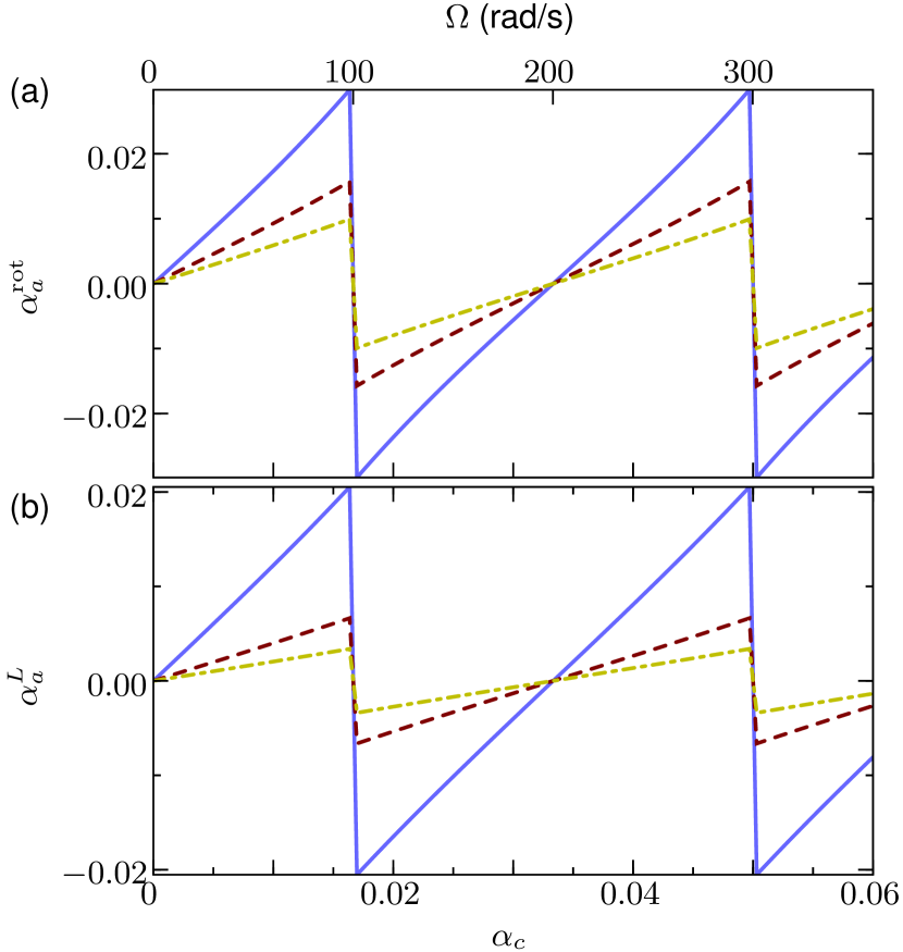
Figure 1: (Color online) Induced phase in the lattice with $30$ lattice sites for (a) a ring rotating with angular speed $\Omega$ and (b) the BEC in a lattice with phase term $\alpha_{c}$. We assume a BEC of ⁸⁷Rb with a linear density $n_{0}=5\times 10^{6}~{}\mathrm{m}^{-1}$. The impurities are ⁸⁷Rb atoms in a different hyperfine level. The lattice spacing is $d=400~{}\mathrm{nm}$, which means that the ring has a circumference of $L=12~{}\mathrm{\mu m}$. In (a) the interspecies coupling strength is $\kappa/2dE_{R}=0.045$, where $E_{R}=\hbar^{2}\pi^{2}/2m_{a}d^{2}$ is the recoil energy of the impurity lattice with impurity mass $m_{a}$, and the curves indicate different BEC couplings $g/2dE_{R}=0.01,0.015,0.02$ (solid, dashed, dashed-dotted lines, respectively). In (b) we assume that both lattices have the same depth, interspecies coupling is $U_{I}/J_{c}=1.5$, and BEC couplings $U_{c}/J_{c}=0.5,1,1.5$ (solid, dashed, and dashed-dotted lines, respectively).

In order to be able to compare our analytical results with numerical solutions we now introduce a system which is numerically solvable beyond the Bogoliubov approximation. This allows us to study the validity of our model of an induced phase beyond the Bogoliubov approximation. We assume that the BEC consisting of $N_{c}$ atoms is trapped in a ring-shaped optical lattice with $N_{s}$ lattice sites and spacing $d$, which is independent of the lattice for the impurities. We will derive an analytical expression for the induced phase in the Bogoliubov approximation, which will have a similar form as the expression in the continuous case of Sec. II.1, Eq. (9). We will use these results for the discussion of the numerical results in Sec. III. One can show that in the limit of $N_{s}\rightarrow\infty$ with $N_{s}d=L=\mathrm{const}$ the two expressions coincide.

The Hamiltonian of the condensate is given by a generalized Bose-Hubbard Hamiltonian Rey et al. (2007)

$$\begin{split}\hat{H}_{BH}&=-J_{c}\sum_{j}\left(\mathrm{e}^{2\pi i\alpha_{c}}\hat{c}_{j+1}^{\dagger}\hat{c}_{j}^{\phantom{\dagger}}+\mathrm{e}^{-2\pi i\alpha_{c}}\hat{c}_{j}^{\dagger}\hat{c}_{j+1}^{\phantom{\dagger}}\right)\\ &\quad+\frac{U_{c}}{2}\sum_{j}^{\phantom{\dagger}}\hat{c}_{j}^{\dagger}\hat{c}_{j}^{\phantom{\dagger}}(\hat{c}_{j}^{\dagger}\hat{c}_{j}^{\phantom{\dagger}}-1),\end{split}$$ (11)

where $J_{c}$ and $U_{c}$ are the hopping and onsite interaction terms of the BEC, respectively, and $\hat{c}_{j}$ is the bosonic annihilation operator for site $j$. For a lattice rotating with angular frequency $\Omega$ the phase factor $\alpha_{c}$ is given by $\alpha_{c}=m_{b}\Omega N_{s}d^{2}/4\pi^{2}\hbar$ Rey et al. (2007). The impurities are trapped in a second lattice as before, for which we assume that it has the same spacing $d$ and the same number of lattice sites $N_{s}$ as the BEC lattice. In this picture the interaction between impurity and BEC atoms is given by

$$\hat{H}_{I}=U_{I}\sum_{j}\hat{n}_{j}\hat{c}_{j}^{\dagger}\hat{c}_{j},$$ (12)

where $U_{I}$ is the coupling strength between the two species. In the remainder of this section we will derive analytically the induced phase of this system resulting from our approximate polaron model. Later we will use Eqs. (11) and (12) for numerical computations of the full two-species model.

Similar to the implementation discussed in the preceding section we now expand the annihilation operators $\hat{c}_{j}$ around an order parameter $\phi_{j}$ as $\hat{c}_{j}=\phi_{j}+\hat{\xi}_{j}$. Then we rewrite this expansion in the momentum representation with quasimomentum $2\pi q/N_{s}$, where $q$ is an integer, and apply a Bogoliubov transformation with quasiparticle operators $\hat{b}_{q}$ and $\hat{b}_{q}^{\dagger}$. For the fluctuations to be small we require that $U_{I}/U_{c}\bar{n}_{0}\ll 1$, where $\bar{n}_{0}=N_{c}/N_{s}$ is the number of BEC atoms per lattice site. The main result is that, as before, we arrive at an effective Hamiltonian of the Hubbard-Holstein form with polarons as the quasiparticles hopping across lattice sites. A derivation of the results is given in the Appendix. In the coherent dynamics limit the Bogoliubov excitations mediate additional interactions and induce a phase in the impurities. The excitations in this system have an energy

$$\hbar\omega_{q}^{L}=E_{q}^{L}+\Lambda_{q},$$ (13)

where $E_{q}^{L}=\sqrt{\epsilon_{q}^{L}(\epsilon_{q}^{L}+2U_{c}\bar{n}_{0})}$, $\Lambda_{q}=-2J_{c}\sin(2\pi q/N_{s})\sin(\Delta\theta/N_{s})$, and $\epsilon_{q}^{L}=4J_{c}\sin^{2}(\pi q/N_{s})\cos(\Delta\theta/N_{s})$. The angle $\Delta\theta$ is determined via the relation $2\pi\alpha_{c}=2\pi\nu/N_{s}+\Delta\theta/N_{s}$ with $\nu$ an integer and $\Delta\theta\in[-\pi,\pi)$. The ground state momentum is determined by the winding number $\nu=\lfloor\alpha_{c}N_{s}\rceil$, where the symbol $\lfloor\cdot\rceil$ denotes rounding to the nearest integer. One can show that the phonon energies in Eq. (13), reduce to the excitation energies of the rotating ring, Eq. (7), in the limit $N_{s}\rightarrow\infty$ with $N_{s}d=L=\text{const}$. The coupling matrix elements between impurities and phonons are given by

$$M_{j,q}^{L}=\frac{U_{I}}{\hbar\omega_{q}^{L}}\sqrt{\frac{\bar{n}_{0}}{N_{s}}}\sqrt{\frac{\epsilon_{q}^{L}}{E_{q}^{L}}}\mathrm{e}^{2\pi iqj/N_{s}}.$$ (14)

From Eq. (5) we calculate the induced phase of the impurity atoms as

$$\alpha_{a}^{L}=\frac{U_{I}^{2}\bar{n}_{0}}{2\pi N_{s}}\sum_{q=1}^{N_{s}-1}\frac{\epsilon_{q}^{L}}{E_{q}^{L}}\frac{1}{(\hbar\omega_{q}^{L})^{2}}\sin(2\pi q/N_{s}).$$ (15)

The form of this induced phase is very similar to the one for a BEC in a rotating ring, Eq. (9). Here however, the cutoff in the phonon quasimomentum is introduced by the quantization of the momentum through the finite lattice. This results in a finite sum instead of a Gaussian depending on the impurity localization width $\sigma$. The reduced hopping term is given by

$$\begin{split}J_{a}^{L}&=\tilde{J}_{a}\exp\Biggl{(}-\frac{U_{I}^{2}\bar{n}_{0}}{N_{s}}\sum_{q=1}^{N_{s}-1}\frac{\epsilon_{q}^{L}}{E_{q}^{L}}\frac{1}{(\hbar\omega_{q}^{L})^{2}}\\ &\quad\times[1-\cos(2\pi q/N_{s})][2N_{q}(T)+1]\Biggr{)}.\end{split}$$

Numerical tests show that the rescaled induced phase $\alpha_{a}^{L}2\pi N_{s}/U_{I}^{2}\bar{n}_{0}$ becomes maximal for $\Delta\theta\rightarrow\pi$ and $U_{c}\bar{n}_{0}\rightarrow 0$. However, Bogoliubov theory loses validity at $\Delta\theta=\pi$ because the ground state becomes degenerate. At small $U_{c}/J_{c}$ we find $\bar{n}_{0}\simeq\bar{n}=N_{c}/N_{s}$ so in order to maximize the constant factor in the induce phase, we have to choose a large filling $\bar{n}$ and large interspecies coupling $U_{I}$. However, the interspecies coupling has to remain sufficiently small to fulfill the condition $U_{I}/U_{c}\bar{n}\ll 1$ that was necessary for the analytical derivation.

In Fig. 1(b) we plot the induced phase according to Eq. (15) for similar parameters as in Fig. 1(a) but now with a BEC in a rotating optical lattice. The induced phase now critically depends on the BEC phase $\alpha_{c}$, which takes the role of the frequency in the preceding section. We observe jumps in the induced phase at critical BEC phases, which have the same origin as the critical frequencies in the rotating ring. The critical phases occur at $\alpha_{\text{crit}}=(2j+1)/2N_{s}$, where $j$ is an integer. We can expect similar orders of magnitude for the induced phase for both setups with or without an optical lattice for the BEC atoms. Note that both the upper and lower x-axes in the figure are valid for both plots because we assume two species of the same mass and the phase in the Bose-Hubbard Hamiltonian $\hat{H}_{BH}$ is a linear function of the frequency.

II.3 The rotating BEC in a static ring

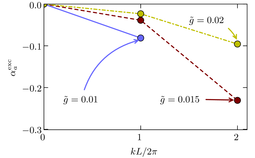
Figure 2: (Color online) Induced phase with a BEC in an excited state. The parameters are the same as in Fig. 1(a) and we abbreviate $\tilde{g}=g/2dE_{R}$. The critical momenta for the different interaction strengths are given by $k_{\text{crit}}L/2\pi\simeq 2.1$, $2.6$, $3.0$ (for $\tilde{g}=0.01,0.015,0.02$, respectively). The lines are only to guide the eye.

Again we consider a quasi-1D BEC in a ring of radius $R=L/2\pi$ and the impurities trapped in a ring-shaped optical lattice immersed into the BEC. In contrast to Sec. II.1, here we assume that the BEC rotates but the ring does not. Hence, the BEC is not in the ground state of the Hamiltonian. This excited state can be created, for example, with a STIRAP process Nandi et al. (2004); Juzeliūnas et al. (2005) or by initializing the BEC in a rotating ring whose rotation is then turned off for the duration of the experiment. The interaction-free Hamiltonian has the same form as the one in the rotating ring, Eq. (6), but with $v=0$. As before we expand the fluctuations around the order parameter in terms of Bogoliubov excitations. The BEC field operator is then given by

$$\hat{\phi}(x)=\mathrm{e}^{ikx}\left[\sqrt{n_{0}}+\sideset{}{{}^{\prime}}{\sum}_{q}\left(u_{q}(x)\hat{b}_{q}-v_{q}^{*}(x)\hat{b}_{q}^{\dagger}\right)\right].$$ (16)

Periodicity requires the quantization of the phase $k=2\pi m/L$ with $m$ an integer. Plugging this ansatz into the GPE results in the chemical potential $\mu_{b}^{\text{exc}}=\hbar^{2}k^{2}/2m_{b}+gn_{0}$. The solutions of the BdG equations diagonalize the quadratic part of the Hamiltonian. In Fetter (1972) they are given as

$$u_{q}(x) =\frac{u_{q}}{\sqrt{L}}\mathrm{e}^{iqx},$$

$$v_{q}(x) =\frac{v_{q}}{\sqrt{L}}\mathrm{e}^{iqx}$$

with the same coefficients $u_{q}$, $v_{q}$ as in the case of a rotating ring [see definition below Eqs. (8)]. The energies of these solutions are given by

$$\hbar\omega_{q}^{\text{exc}}=E_{q}^{B}+\hbar qw,$$

where $w=\hbar k/m_{b}$ is the speed associated with momentum $k$. For $\hbar\omega_{q}^{\text{exc}}$ to be positive we have assumed that the velocity of the BEC is less than the speed of sound, i.e., $w<c$, which is equivalent to a critical momentum $k_{\text{crit}}=1/\xi_{h}$. Again we assume that the impurity wave function is given by a Gaussian centered at the position $x_{j}$ of lattice site $j$. This allows us to evaluate the induced phase as

$$\alpha_{a}^{\text{exc}}=\frac{\kappa^{2}n_{0}}{2\pi L}\sideset{}{{}^{\prime}}{\sum}_{q}\frac{\epsilon_{q}^{0}}{E_{q}^{B}}\frac{1}{(\hbar\omega_{q}^{\text{exc}})^{2}}\mathrm{e}^{-q^{2}\sigma^{2}/2}\sin(qd).$$

We see that the form of this phase is the same as in Eq. (9) but now the phonon energy depends on the full momentum of the BEC $k$, not only the mismatch to the ground state $\Delta k$. Similarly, the form of the reduced hopping is the same as Eq. (10) but with $\hbar\omega_{q}^{\text{rot}}$ replaced by $\hbar\omega_{q}^{\text{exc}}$. The higher energies allow for larger induced phases but entail the experimental difficulty of maintaining the BEC in an excited state Ögren and Kavoulakis (2009); Ryu et al. (2007). A derivation of the life time of this excited state is beyond the scope of the present work.

Figure 2 shows the induced phase in this setup for experimentally accessible parameters below the critical momentum. Induced phases up to $\alpha_{a}^{\text{exc}}\simeq-0.25$ are readily achievable in this setup and even higher phase are possible by slightly changing the parameters. The reason for the negative sign of the phase is that the dispersion favors phonons with negative quasimomentum. A negative quasimomentum, i.e., total phonon quasimomentum $k-|q|$, pushes the system closer to the ground state at zero total momentum.

III Probing the phase twist

In Klein and Jaksch (2009) it was shown that the presence of a phase twist in the impurity Hamiltonian can be observed as a drift of the impurities. If we prepare a Gaussian-shaped distribution of impurity atoms centered at lattice site $j$, then it will expand and the mean position of this packet will drift either to the left or right depending on the induced phase. This drift can be verified experimentally. It is also present for impurity speeds below the speed of sound, which, at first glance, seems to contradict the Landau criterion of superfluid flow Landau (1941); Leggett (1999). From this criterion one would expect that a BEC rotating below the Landau critical speed does not impart a momentum on the impurity. Recent work by Sykes et al. Sykes et al. (2009) and earlier works by Roberts et al. Roberts and Pomeau (2005); Roberts (2006) suggest Doppler-shifted scattering processes of quantum fluctuations in the BEC with the impurity as a source for this drift. When an incoming wave of a BEC quantum fluctuation is reflected off an impurity it experiences a Doppler shift depending on the propagation direction, which leads to an overall drag force on the impurity. In contrast to their derivation, our results are based on the nonperturbative Lang-Firsov transformation and we assume periodic boundary conditions.

In the remainder of this section, we present detection methods for the induced phase twist, namely, via mass current measurements and ToF expansion. In order to compare the effective one-species model, Eq. (4), with numerical results we use a two-species Bose-Hubbard Hamiltonian $\hat{H}_{2BH}=\hat{H}_{a}+\hat{H}_{BH}$, which can be solved by numerical diagonalization for small systems.

III.1 Impurity ground state momentum

For a single impurity our effective one-species model predicts a vanishing ground state momentum for $|\alpha_{a}|<1/2N_{s}$. In the full two-species model interactions between the two atom species cause a broadening of the reduced impurity ground state in momentum space even for a single impurity. We now investigate how this broadening can be used to measure the induced phase $\alpha_{a}$ of our effective model. For vanishing induced phase the broadening in momentum space is symmetric around the zero momentum state. However, for $0<|\alpha_{a}|<1/2N_{s}$ the broadening becomes asymmetric around the zero momentum state. This leads to a small nonvanishing mean momentum of the impurity ground state. We note that the origin of this effect is different from the expected jump of the momentum ground state at the critical phases $\alpha_{\text{crit}}$. At a critical phase the macroscopic occupation of a momentum state changes, whereas the asymmetric broadening is a perturbative effect and does not cause such a macroscopic shift. To see this effect analytically we calculate the ground state of the Hubbard-Holstein Hamiltonian, Eq. (3), in first-order Rayleigh-Schrödinger perturbation theory for a single impurity Kuper and Whitfield (1963). For simplicity we let $\bar{E}_{j}=0$ and $\tilde{\mu}_{a}=0$ so that we can rewrite Eq. (3) in momentum space as $\hat{H}_{\text{HH}}=\sum_{k}E_{k}^{a}\hat{a}_{k}^{\dagger}\hat{a}_{k}^{\vphantom{\dagger}}+\sideset{}{{}^{\prime}}{\sum}_{q}\hbar\omega_{q}^{\text{rot}}\hat{b}_{q}^{\dagger}\hat{b}_{q}^{\vphantom{\dagger}}+\sideset{}{{}^{\prime}}{\sum}_{q,k}\hbar\omega_{q}^{\text{rot}}M_{q}^{\text{rot}}\left(\hat{b}_{q}^{\vphantom{\dagger}}\hat{a}_{k+q}^{\dagger}\hat{a}_{k}^{\vphantom{\dagger}}+\hat{b}_{q}^{\dagger}\hat{a}_{k-q}^{\dagger}\hat{a}_{k}^{\vphantom{\dagger}}\right)$, where $\hat{a}_{k}$ annihilates an impurity with quasimomentum $k$, $E_{k}^{a}=-2\tilde{J}_{a}\cos(kd)$ is the unperturbed impurity dispersion with quasimomentum $k$, and $M_{q}^{\text{rot}}$ is the Fourier-transformed coupling matrix element $M_{j,q}$. The coupling term mixes phonon and impurity excitations. We write the unperturbed states as $\ket{k,N_{q}}$, which indicates an impurity with quasimomentum $k$ and $N_{q}$ Bogoliubov excitations with quasimomentum $q$. With this notation the perturbed (dressed) ground state is

$$\ket{k_{0},0}^{(1)}=\ket{k_{0},0}+\sideset{}{{}^{\prime}}{\sum}_{q}\frac{\hbar\omega_{q}M_{q}}{E^{a}_{k_{0}}-E^{a}_{k_{0}-q}-\hbar\omega_{q}}\ket{k_{0}-q,1_{q}},$$

where $k_{0}$ is the quasimomentum of the impurity ground state. The quasimomentum distribution $n_{k}$ and mean quasimomentum $\bar{k}$ of this state are given by

$$n_{k} =\langle\hat{a}_{k}^{\dagger}\hat{a}_{k}\rangle=\delta_{kk_{0}}+\left(\frac{\hbar\omega_{k_{0}-k}|M_{k_{0}-k}|}{E^{a}_{k_{0}}-E^{a}_{k}-\hbar\omega_{k_{0}-k}}\right)^{2},$$ (17)

$$\bar{k} =\sum_{k}n_{k}k.$$ (18)

To be able to compare the numerically obtained mean quasimomentum with this formula we insert the expression for $M_{k}$ for the BEC in an optical lattice, Eq. (14), into Eq. (17). Moreover, in a lattice the quasimomentum $k$ is expressed as $2\pi k/N_{s}$, where $k$ is now an integer. With the resulting quasimomentum distribution $n_{k}$ the mean quasimomentum, Eq. (18), reads

$$\bar{k}=-\frac{U_{I}^{2}\bar{n}_{0}}{N_{s}}\sideset{}{{}^{\prime}}{\sum}_{k=-\lfloor N_{s}/2\rceil+1}^{\lfloor N_{s}/2\rceil-1}\frac{\epsilon_{k}^{L}}{E_{k}^{L}}\frac{2\pi k/N_{s}}{\left(E^{a}_{0}-E^{a}_{k}-\hbar\omega_{k}^{L}\right)^{2}},$$ (19)

where we have used the fact that $\epsilon_{k}^{L}$, $E_{k}^{L}$, and $E_{k}^{a}$ are even functions of $k$. This expression should be compared to the expression for the induced phase, Eq. (15). The sine in Eq. (15) can be linearized for $2\pi q/N_{s}$ close the roots of the sine. Furthermore, the summation indices of both expressions can be shifted so that the two expressions formally coincide apart from the different energy denominators and a constant. To analyze the energy denominator in Eq. (19) we assume $U_{c}=0$ for clarity. Then it is given by $E^{a}_{0}-E^{a}_{k}-\hbar\omega^{L}_{k}=-2(\tilde{J}_{a}+J_{c})[1-\cos(2\pi k/N_{s})]-\Lambda_{k}\simeq-\hbar\omega^{L}_{k}(1+\tilde{J}_{a}/J_{c})$ for phases $\alpha_{c}$ close to $j/N_{s}$ ($j$ integer), that is small $\Lambda_{k}$. We might thus expect that

$$\bar{k}\simeq-\frac{2\pi}{(1+\tilde{J}_{a}/J_{c})^{2}}\alpha_{a}^{L}.$$ (20)

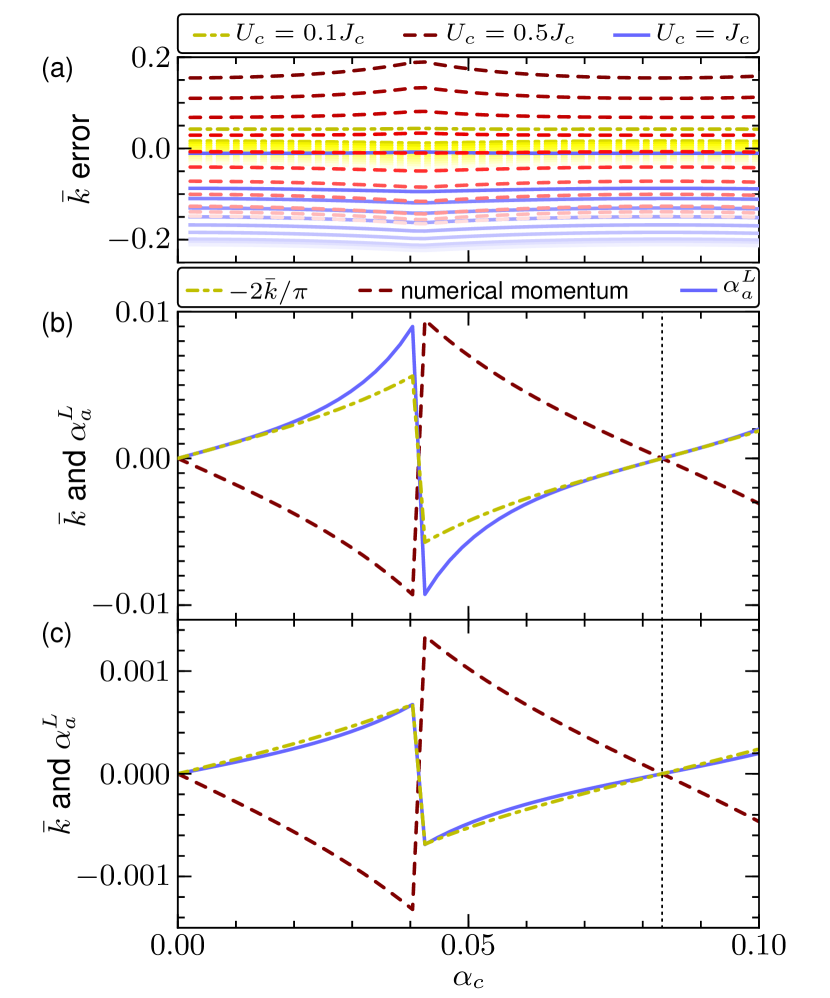
Figure 3: (Color online) (a) Relative error $\bar{k}_{\text{ana}}/\bar{k}_{\text{num}}-1$ of Eq. (19) compared to the numerically exact ground state quasimomentum for different interactions at $N_{s}=12$, $6$ BEC atoms, and one impurity with $\tilde{J}_{a}=J_{c}$. Line styles indicate different BEC interactions $U_{c}$ (see legend) and increasing lightness (from top to bottom) indicates decreasing interspecies coupling $U_{I}/J_{c}\in\{0.2,0.15,0.14,\dots,0.05,0.01\}$ (dashed-dotted lines), $\{0.9,0.8,\dots,0.1,0.05,0.01\}$ (dashed), $\{1,0.7,0.6,\dots,0.1,0.05,0.01\}$ (solid). (b)–(c) Comparison of analytical induced phase (solid), numerically exact mean quasimomentum (dashed) and the rescaled analytical mean quasimomentum $-2\bar{k}/\pi$ (dashed-dotted) for (b) $U_{c}=0.5J_{c}$, $U_{I}=0.4J_{c}$ and (c) $U_{c}=J_{c}$, $U_{I}=0.2J_{c}$. The rescaling factor $-2/\pi$ results from Eq. (20). The dotted vertical line indicates $\alpha_{c}=1/N_{s}$.

In order to check the validity of these approximations we have computed ground states of the two-species Bose-Hubbard Hamiltonian with a single impurity. From the reduced density matrix of the impurity we compute the mean quasimomentum and compare it with Eq. (19). Figure 3(a) shows the error of the formula (19) relative to the numerical results for different sets of interactions. As expected, the accuracy of the analytical result is better for small interactions (e.g., approximately $\pm 5\%$ for $U_{c}=0.1J_{c}$). In Fig. 3(b)–(c) we compare the mean quasimomentum of the impurity ground state with the analytical result for the induced phase, Eq. (15). Clearly, our approximations discussed in the preceding paragraph predict the value of the induced phase for $\alpha_{a}^{L}$ close to $\alpha_{c}=j/N_{s}$ ($j$ integer), that is away from the critical phases $\alpha_{\text{crit}}=(2j+1)/2N_{s}$, where Bogoliubov theory fails. Also note that in Fig. 3(b) the constraints on the validity of our analytical derivation of the induced phase are not met ($U_{I}\not\ll U_{c}\bar{n}_{0}$). Nevertheless, the rescaled mean quasimomentum approximates the induced phase well close to the roots of $\alpha_{a}^{L}$, which means that qualitatively our effective polaron model still describes the underlying physics.

Our computational resources restrict the size of the systems studied here to moderately small number of lattice sites and filling factors. Therefore, we could not directly observe the jump of the impurity to a macroscopic occupation of a nonzero momentum ground state for $\alpha_{a}^{L}>\alpha_{\text{crit}}$. However, our results clearly indicate an imbalanced momentum distribution owing to the influence of an induced phase. For larger number of lattice sites the critical phase $\alpha_{\text{crit}}$ decreases. Furthermore, the quantization of the impurity ground state momentum in units of $2\pi/N_{s}$ becomes denser for larger lattices so that more allowed momentum states become available for the impurity. Therefore, we expect to see a macroscopic population of a nonzero momentum state in larger systems caused by a large induced phase as predicted by our effective model. Such a macroscopic population will be observable as an impurity current in an experiment. The current measured by the operator

$$\hat{C}_{a}=\frac{i\tilde{J}_{a}m_{a}}{\hbar}\sum_{j}\left(\hat{a}_{j+1}^{\dagger}\hat{a}_{j}^{\phantom{\dagger}}-\hat{a}_{j}^{\dagger}\hat{a}_{j+1}^{\phantom{\dagger}}\right)$$

is closely related to the mean momentum of the impurity. It is straightforward to show that the current of a single impurity with momentum $\bar{k}$ is $\langle\hat{C}_{a}\rangle=2\tilde{J}_{a}m_{a}\sin(2\pi\bar{k})/\hbar$. For small $\bar{k}$ as in Fig. 3 we may approximate $\langle\hat{C}_{a}\rangle\propto\sin(2\pi\bar{k})\simeq 2\pi\bar{k}$. In the preceding paragraph we have seen that close to the zero crossing the induced phase and mean momentum are proportional, which shows that the induced phase and the mass current measured by $\hat{C}_{a}$ are proportional around $\alpha_{c}=1/N_{s}$.

III.2 Time of flight images

Another experimentally readily accessible method to probe for a phase term is the ToF expansion of the atoms. After their evolution the atoms are abruptly released from the trap and expand for a time $t$ before they are imaged. If interactions can be neglected during the time of flight, the imaged density distribution corresponds to the momentum distribution of the atoms in the trap. This distribution at a position $\mathbf{x}$ is given by

$$\rho_{\text{ToF}}(\mathbf{x})=|\tilde{w}(\mathbf{K})|^{2}\sum_{j_{1},j_{2}}\rho_{1}(\mathbf{R}_{j_{1}},\mathbf{R}_{j_{2}})\mathrm{e}^{i\mathbf{K}\cdot(\mathbf{R}_{j_{1}}-\mathbf{R}_{j_{2}})},$$

where we neglect a constant factor $(m_{a}/\hbar t)^{3}$ Bloch et al. (2008). In the ballistic approximation the momentum is $\mathbf{K}=m_{a}\mathbf{x}/\hbar t$ with $m_{a}$ the mass of an impurity atom, and $\tilde{w}(\mathbf{K})$ the Fourier transform of the Wannier function of the impurity trapped in an optical lattice. The one-particle density matrix is given by $\rho_{1}(\mathbf{R}_{j_{1}},\mathbf{R}_{j_{2}})=\langle\hat{a}_{\mathbf{R}_{j_{1}}}^{\dagger}\hat{a}_{\mathbf{R}_{j_{2}}}^{\phantom{\dagger}}\rangle$, where $\hat{a}^{\dagger}_{\mathbf{R}_{j}}$ creates an impurity atom at position $\mathbf{R}_{j}$. In a ring of radius $R$ the positions $\mathbf{R}_{j}$ are fixed at $\mathbf{R}_{j}=R[\sin(2\pi j/N_{s}),\cos(2\pi j/N_{s})]$. For tightly localized atoms we can set $\tilde{w}(\mathbf{K})=1/\sqrt{N_{s}}$ and write

$$\begin{split}\rho_{\text{ToF}}(\mathbf{x})&=\frac{1}{N_{s}}\sum_{j_{1},j_{2}}\rho_{1}(\mathbf{R}_{j_{1}},\mathbf{R}_{j_{2}})\\ &\quad\times\exp\{iK_{x}R[\sin(2\pi j_{1}/N_{s})-\sin(2\pi j_{2}/N_{s})]\\ &\qquad+iK_{y}R[\cos(2\pi j_{1}/N_{s})-\cos(2\pi j_{2}/N_{s})]\}.\end{split}$$

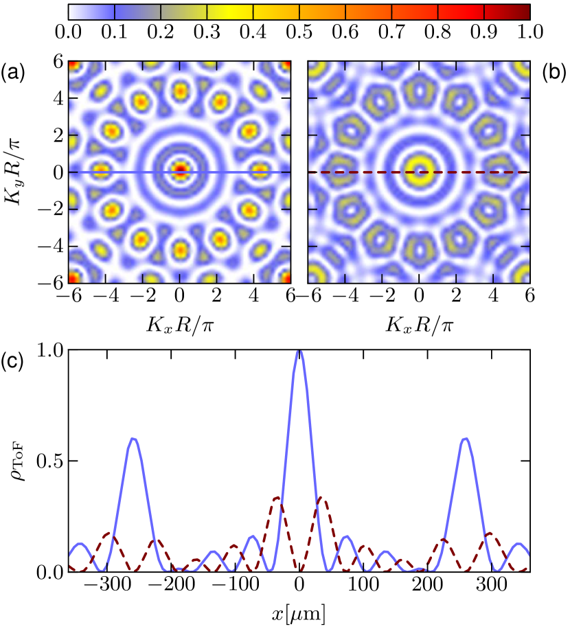
Figure 4: (Color online) Time of flight distribution $\rho_{\text{ToF}}$ of a single impurity released from a ring lattice with $N_{s}=12$ at $T=0$ in the single-species model, Eq. (4). The central peak in (a) indicates a zero quasimomentum ground state for $\alpha_{a}=0.04$. In (b) the vanishing density in the center indicates that the ground state exhibits nonzero momentum ($\alpha_{a}=0.05$). The jump between these two momentum states occurs at $\alpha_{a}=1/2N_{s}\simeq 0.042$. In (c) we show the corresponding density profiles indicated with horizontal lines in (a) and (b). The ToF expansion time is $t=50~{}\mathrm{ms}$ for ⁸⁷Rb atoms in a ring of radius $R=12\mu\mathrm{m}$.

To illustrate the effect of an induced phase term in the effective impurity Hamiltonian, Eq. (4), we first consider the ToF expansion of a single atom, which is not immersed in a BEC. While this atom alone without a surrounding BEC would not exhibit a phase term in practice, it is possible to include this phase term in the numerical calculation to illuminate its effect. We will study the full two-species system in the next paragraph. We have seen in the preceding sections that the critical phases $\alpha_{\text{crit}}$ correspond to a macroscopic jump in the momentum of the ground state. As a consequence, if the induced phase crosses $\alpha_{\text{crit}}$, the ground state of the impurity will jump to a higher momentum state. Since the ToF distribution represents the momentum distribution of the trapped atoms, we expect a central peak for nonrotating impurities and a vanishing density at the center for impurities with a nonzero momentum Cozzini et al. (2006); Nunnenkamp et al. (2008). ToF images can reveal this jump in the momentum of the impurity with good accuracy. Corresponding density plots are shown in Fig. 4(a) for a phase below and in Fig. 4(b) for a phase above the lowest critical phase $\alpha_{\text{crit}}=1/2N_{s}$. In Fig. 4(c) we plot the profiles of the density distribution after a realistic time of flight. The different profiles of the two ToF images should be clearly distinguishable with typical camera resolutions Nelson et al. (2007).

Figure 5: (Color online) Influence of temperature on the ToF images in the two-species Bose-Hubbard model. A single impurity is submerged into a BEC with $6$ atoms in $N_{s}=12$ lattice sites, hopping $\tilde{J}_{a}=J_{c}$, interspecies coupling $U_{I}=0.5J_{c}$, BEC interaction $U_{c}=0.4J_{c}$, and BEC phase $\alpha_{c}=0.042$. In (a) $k_{B}T=0$ and in (b) $k_{B}T=2J_{c}$.

We now return to the numerical study of the full two-species Bose-Hubbard model with a rotating BEC and a stationary impurity lattice. For the moderately small system sizes studied here we cannot expect to see a clear transition to a macroscopic occupation of a nonzero impurity momentum state because the induced phase is not sufficiently large to cause this jump. Instead, in Fig. 5 we show the influence of nonzero temperature on the central peak in the ToF image of the impurity. The BEC phase is chosen to be close to the critical phase $1/2N_{s}$ so that the induced phase is expected to be large. The density distribution in Fig. 5(a) is very similar to the single-species calculation in Fig. 4(a), which means that small interspecies interactions do not influence the ToF image significantly. However, the induced phase is not sufficiently large to cause a macroscopic occupation of a nonzero momentum state as revealed by a vanishing central density in Fig. 4(b). This is consistent with our analytical formula of the effective polaron model, Eq. (15), which does predict an induced phase below the critical phase $1/2N_{s}$ for the parameters used in Fig. 5. In Fig. 5(b) we have chosen the same parameters as in Fig. 5(a) but with a large temperature. The finite temperature in this plot manifests itself in a thermal background distribution superimposed on the coherent distribution, which reduces the contrast of the ToF image. However, even at such large temperatures the features of the distribution are still visible and we expect this method to be able to distinguish between the distributions with a central peak or a central dip at typical experimental temperatures.

An application of this phase detection method via ToF images might be to use the impurity as a nondestructive probe to reveal the rotational state of the underlying BEC. If the rotation is sufficiently close to a critical phase, the probe will acquire a phase which is detected by the central dip in the ToF image.

IV Clustering of impurity atoms

The presence of the coherent phonon cloud surrounding the lattice atoms mediates a long-range interaction between distant atoms. Furthermore, the onsite interaction decreases with the polaronic level shift $E_{p}$. For a sufficiently large mediated interaction this can result in an attractive onsite potential Klein et al. (2007). In this section, we will see how a phase twist influences the clustering properties of the impurities. All computations in this section are based on numerically exact diagonalization of either the one- or two-species Bose-Hubbard Hamiltonian.

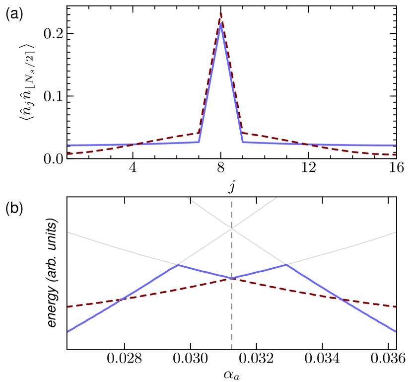
Figure 6: (Color online) (a) Correlations of impurities for $N_{s}=16$ lattice sites, $3$ atoms, and $U_{a}=-0.125\tilde{J}_{a}$. The two lines represent the two families of correlations depending on the momentum state of the system, i.e., the phase $\alpha_{a}$. Each family is a set of correlations for many values of $\alpha_{a}$. (b) The spectrum exhibits crossings below and above the critical phases $\alpha_{\text{crit}}$ (the first critical phase is indicated with a vertical dashed line), where the impurities switch their momentum ground state (thick solid and dashed lines). The thin gray lines indicate higher lying energy levels.

We study the effective single-species Bose-Hubbard model, Eq. (4), which contains a phase term $\alpha_{j,j^{\prime}}=\alpha_{a}$ in the hopping, and assume an attractive interaction ($U_{a}/\tilde{J}_{a}<0$). The effect of the mediated interaction is measured by the density-density correlation $\langle\hat{n}_{j}\hat{n}_{j^{\prime}}\rangle$ between sites $j$ and $j^{\prime}$. In Fig. 6(a) we see the effect of the phase term on the density-density correlations $\langle\hat{n}_{j}\hat{n}_{\lfloor N_{s}/2\rceil}\rangle$. Depending on the value of the induced phase the ground state is either in a weakly or a more strongly bound state. The strongly bound state with a higher onsite correlation is observed when the ground state of the system changes its momentum. In the energy spectrum this switch corresponds to a crossing of the two lowest energy levels. The energy spectrum of the system in Fig. 6(b) shows such crossings close to the first critical phase $\alpha_{\text{crit}}=1/2N_{s}$. We find two such crossings below and above each critical phase. For the values of $\alpha_{a}$ in between two such crossings the ground state becomes stronger bound. Thus the two families of correlations indicated in Fig. 6(a) consist of the correlations for all $\alpha_{a}$ either between two crossing above and below a critical phase or outside the crossing region. For different sets of parameters the picture may feature more than two differently bound sets of states depending on the number of crossings within the lowest energy level. In conclusion, the effect of a phase term in the attractive Bose-Hubbard model is to introduce energy crossings and to bind the atoms more strongly for certain values of the phase.

V Quantum chaos

We now briefly address the question if our system exhibits quantum chaotic behavior as observed recently for a single-mode Bose-Hubbard model with a phase twist Buonsante and Wimberger (2008). In our two-component Bose-Hubbard model, the phase of the second component is induced through coupling with the first component. This is different from the one-species model, where such an interspecies coupling is not present and where a phase term has to be assumed a priori. To formalize the notion of quantum chaos we denote with $\Delta E_{j}$ the distance between two neighboring energy levels $E_{j}$ and $E_{j+1}$, and with $\overline{\Delta E}$ the average over all spacings $\Delta E_{j}$. Furthermore, we define a quasi-continuous parameter $s=\Delta E/\overline{\Delta E}$ for the normalized energy spacings. Then a nonchaotic system follows the Poisson distribution with a probability density $p(s)=\exp(-s)$. On the other hand, a quantum chaotic system follows a GOE distribution $p(s)=\pi s\exp(-\pi s^{2}/4)/2$. The repulsion of levels expressed in the GOE is a result of correlations in the system, which are not present in the uncorrelated Poissonian (nonchaotic) statistics.

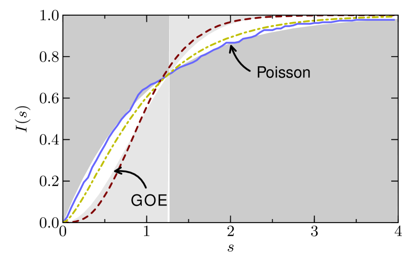
Figure 7: (Color online) Cumulative level spacing for different disorder strengths $e/J_{c}=0,1,20$ (solid blue, dashed red, dashed-dotted yellow lines, respectively). The edge of the dark shaded area indicates the Poisson prediction and the light shaded area the GOE prediction. The curves describe a crossover from regular behavior to chaotic, and back to regular for increasing disorder. This is for $3$ BEC atoms and $2$ impurities in lattices with $5$ sites averaged over $100$ independent disorder realizations. The other parameters are $U_{c}=1.5J_{c}$, $U_{a}=0.1J_{c}$, $U_{I}=J_{c}$, $\alpha_{c}=0.057$.

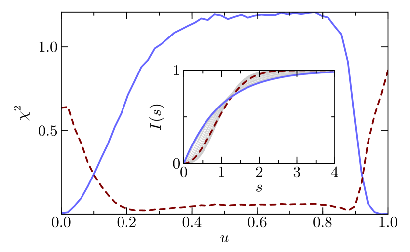
Figure 8: (Color online) $\chi^{2}$ tests of the Poisson (solid line) and GOE predictions (dashed line). For intermediate values of $u$ ($0.2\lesssim u\lesssim 0.9$) the energy distribution closely follows the GOE prediction. Below and above these values we observe a more regular behavior as the system is in either the hopping-only or the no-hopping state, respectively. As parameters we have chosen $N_{s}=5$ lattice sites, $3$ BEC atoms, $2$ impurities, $\alpha_{c}=0.057$. The results have been averaged over $100$ independent disorder realizations. The inset shows the individual cumulative level distributions (thin lines, which appear as a gray area at this resolution) together with the Poisson (solid line) and GOE predictions (dashed line).

Because of the various symmetries in the Bose-Hubbard model one cannot expect a global quantum chaotic behavior of such a system. One approach is to restrict oneself to the local behavior in suitable subspaces which do not exhibit these symmetries Kolovsky and Buchleitner (2004). Another approach—and typically easier to achieve in experiments—is to break symmetries explicitly, for example, breaking translational symmetry by introducing random disorder Buonsante and Wimberger (2008). We introduce disorder into the two-component Bose-Hubbard Hamiltonian with a phase twist by adding a local term with a random strength

$$\hat{H}_{\text{dis}}=\sum_{j}\left(e_{j}^{\vphantom{\dagger}}\hat{c}_{j}^{\dagger}\hat{c}_{j}^{\phantom{\dagger}}+e_{j}^{\prime}\hat{a}_{j}^{\dagger}\hat{a}_{j}^{\phantom{\dagger}}\right).$$

The energies $e_{j}$ and $e_{j}^{\prime}$ are two independent random variables uniformly distributed on an interval $(-e/2,e/2)$. In Fig. 7 we plot the integrated level distribution $I(s)=\int_{0}^{s}p(s^{\prime})ds^{\prime}$ for different values of the disorder strength $e$. For vanishing disorder, the system follows closely the regular behavior of the Poisson distribution. Choosing the same order of magnitude for all energy scales $J_{a,c}\simeq U_{a,c}\simeq U_{I}\simeq e$ we recover a similar behavior as observed in the one-component Bose-Hubbard model in Buonsante and Wimberger (2008). The energy level distribution follows most closely the distribution of a GOE, which indicates quantum chaos. Increasing the disorder further reestablishes the regular behavior because the atoms tend to localize in the disorder potential. The effect of the interspecies interaction on the level spacing is investigated in Fig. 8. There we have defined a parameter $u=U_{I}/e=U_{a,c}/e$ with $J_{a,c}/e=1-u$. As we sweep $u$ from $0$ to $1$, the underlying Hamiltonian changes from describing an ideal two-component system with hopping to a fully interacting system without hopping. In the absence of the disorder potential these two extremal cases would lead to degenerate eigenenergies (going from momentum Fock eigenstates to spatial Fock states). Disorder lifts the degeneracy and we can observe global quantum chaotic behavior. We recover very similar curves with the definition $u=U_{I}/e$ and $J_{a,c}/e=U_{a,c}/e=1-u$. The $\chi^{2}$ tests plotted in Fig. 8 indicate that the system initially follows a regular behavior but quickly changes to a GOE distribution. Increasing the interaction further, ultimately the behavior becomes regular again in the no-hopping regime. We have defined $\chi^{2}=\sum_{j}[I_{\text{num}}(s_{j})-I(s_{j})]^{2}$, where $I_{\text{num}}(s_{j})$ are the numerically obtained cumulative level spacings at point $s_{j}$ and $I(s_{j})$ is either the integrated Poisson or GOE distribution.

VI Conclusion

We have presented a method for creating an artificial magnetic field in a ring of trapped neutral atoms. Our method works by submerging atoms trapped in an optical lattice into a BEC which exhibits a phase term. We have discussed different setups which lead to an induced phase in the impurities. First, with a BEC in a rotating ring, second, with a rotating BEC in a static ring. We have then derived an effective polaron model, which reduces the problem to a single-species Hubbard model with a phase term on the hopping. For realistic parameters our analytical formulas predict induced phases up to $\alpha_{a}\simeq 0.03$ in the first setup or $|\alpha_{a}|\simeq 0.25$ with a BEC in an excited rotational state. Comparisons with numerical solutions of the full problem for small systems show that our model can be used to qualitatively describe the system even beyond the constraints set by the analytical derivation. Furthermore, we have discussed methods for observing the induced phase in the impurities: by using ToF images and measuring mass currents. The ToF images show a sharp transition when a critical value of the induced phase is crossed. Increasing temperature or interspecies coupling obscures the sharp transition but the main features of the transition remain observable. Finally, we have compared and extended studies of quantum chaos to the two-species Bose-Hubbard Hamiltonian with a phase twist. By introducing random disorder we could observe the onset of chaos when all energy scales in the system are of the same order, similar to the result of a one-species Bose-Hubbard Hamiltonian with a phase twist. In the two-species model the interspecies coupling ensures that the impurities exhibit a nontrivial phase, which is necessary to observe quantum chaos in this model.

Contemporary optical lattice technology allows the investigation of large systems of coherent neutral atoms evolving under a precisely known Hamiltonian, which is often not the case in actual condensed matter experiments. The methods presented here can be seen as a simulation of the effects of magnetic fields on ring systems. However, the 1D treatment also allows us to gain insight into a 2D system of impurities immersed into a rotating 2D BEC Klein and Jaksch (2009). Our results suggest that, in general, one may expect a decrease in the induced phase for nonvanishing interaction in 2D. However, the reduction is not expected to destroy the large phases obtainable in 2D. Furthermore, detection methods similar to the ones presented here will be applicable in the 2D setup. In 2D a phase in the hopping term of the Bose-Hubbard Hamiltonian gives rise to the quantum Hall effect Palmer and Jaksch (2006). In light of this prospect, an extension of our methods to 2D will be of great interest and offer a quantum simulator for even more condensed matter models.

*

Appendix A Bogoliubov approximation in the lattice with a phase twist

To derive the Bogoliubov excitations for a BEC in a 1D lattice with a phase term in the hopping we follow van Oosten et al. (2001), where the authors derive the Bogoliubov approximation for a Bose-Hubbard model without a phase twist. First, we include the chemical potential $\mu_{c}^{L}$ in the Bose-Hubbard Hamiltonian, Eq. (11),

$$\begin{split}\hat{H}_{BH}&=-J_{c}\sum_{j}\left(\mathrm{e}^{2\pi i\alpha_{c}}\hat{c}_{j+1}^{\dagger}\hat{c}_{j}^{\phantom{\dagger}}+\mathrm{e}^{-2\pi i\alpha_{c}}\hat{c}_{j}^{\dagger}\hat{c}_{j+1}^{\phantom{\dagger}}\right)\\ &\quad+\frac{U_{c}}{2}\sum_{j}^{\phantom{\dagger}}\hat{c}_{j}^{\dagger}\hat{c}_{j}^{\phantom{\dagger}}(\hat{c}_{j}^{\dagger}\hat{c}_{j}^{\phantom{\dagger}}-1)-\mu_{c}^{L}\sum_{j}\hat{c}_{j}^{\dagger}\hat{c}_{j}^{\phantom{\dagger}}.\end{split}$$ (21)

We rewrite this Hamiltonian in the momentum representation with $\hat{c}_{j}=(1/\sqrt{N_{s}})\sum_{q}\hat{d}_{q}\mathrm{e}^{i2\pi qj/N_{s}}$. Noting that $\sum_{j}\mathrm{e}^{i2\pi j(q-q^{\prime})/N_{s}}=N_{s}\delta_{q,q^{\prime}}$ we arrive at

$$\begin{split}\hat{H}_{BH}&=\sum_{q}\left(\bar{\epsilon}_{q}^{L}-\mu_{c}^{L}\right)\hat{d}_{q}^{\dagger}\hat{d}_{q}^{\phantom{\dagger}}\\ &\quad+\frac{U_{c}}{2N_{s}}\sum_{q,q^{\prime},q^{\prime\prime},q^{\prime\prime\prime}}\hat{d}_{q}^{\dagger}\hat{d}_{q^{\prime}}^{\dagger}\hat{d}_{q^{\prime\prime}}^{\phantom{\dagger}}\hat{d}_{q^{\prime\prime\prime}}^{\phantom{\dagger}}\delta_{q+q^{\prime},q^{\prime\prime}+q^{\prime\prime\prime}},\end{split}$$

where $\bar{\epsilon}_{q}^{L}=-2J_{c}\cos(2\pi q/N_{s}-\theta)$ and $\theta=2\pi\alpha_{c}$. For the case considered in Sec. II.2 the BEC is assumed to be in the ground state with integer winding number $q_{0}$, which minimizes the energy $\bar{\epsilon}_{q}^{L}$. We therefore write $\theta=2\pi q_{0}/N_{s}+\Delta\theta/N_{s}$, where $\Delta\theta\in[-\pi,\pi)$ determines the mismatch of the externally given phase twist $\theta$ and the phase of the ground state. The ground state energy is then given by $\bar{\epsilon}_{q_{0}}^{L}=-2J_{c}\cos(\Delta\theta/N_{s})$.

The ground state is occupied with a macroscopically large number of atoms in mode $q_{0}$, that is $\langle\hat{d}_{q_{0}}^{\dagger}\hat{d}_{q_{0}}^{\phantom{\dagger}}\rangle\simeq\langle\hat{d}_{q_{0}}^{\phantom{\dagger}}\hat{d}_{q_{0}}^{\dagger}\rangle\sim N_{0}$ and all other momentum state densities with $q\neq q_{0}$ are negligible. This allows us to rewrite the creation and annihilation operators in terms of a mean field contribution and quantized fluctuations, that is

$$\hat{d}_{q_{0}},\hat{d}_{q_{0}}^{\dagger} \rightarrow\sqrt{N_{0}},$$

$$\hat{d}_{q}^{\phantom{\dagger}},\hat{d}_{q}^{\dagger} \rightarrow\hat{d}_{q}^{\phantom{\dagger}},\hat{d}_{q}^{\dagger}\quad\text{for }q\neq q_{0}.$$

The chemical potential attains a value such that the Hamiltonian is minimal with respect to $N_{0}$. It is given by $\mu_{c}^{L}=\bar{\epsilon}_{q_{0}}^{L}+U_{c}\bar{n}_{0}$, where $\bar{n}_{0}=N_{0}/N_{s}$ is the density of the condensed atoms. An effective Hamiltonian is derived by only keeping terms up to second order in the fluctuations. For the second order part we keep two operators and replace the respective other two by $N_{0}$ in the interaction terms of the Hamiltonian. Furthermore, we substitute the chemical potential and use the bosonic commutation relation $[\hat{d}_{q}^{\phantom{\dagger}},\hat{d}_{q}^{\dagger}]=1$. This procedure yields the Hamiltonian

$$\begin{split}\hat{H}^{(0+2)}&=-\frac{1}{2}U_{c}\bar{n}_{0}N_{0}-\frac{1}{2}\sideset{}{{}^{\prime}}{\sum}_{q}\left(\bar{\epsilon}_{q}^{L}-\bar{\epsilon}_{q_{0}}^{L}+U_{c}\bar{n}_{0}\right)\\ &\quad+\frac{1}{2}\sideset{}{{}^{\prime}}{\sum}_{q}\left(\hat{d}_{q_{0}+q}^{\dagger},\hat{d}_{q_{0}-q}^{\phantom{\dagger}}\right)D\begin{pmatrix}\hat{d}_{q_{0}+q}\\ \hat{d}_{q_{0}-q}^{\dagger}\end{pmatrix},\end{split}$$

where

$$D=\begin{pmatrix}\tilde{\epsilon}_{q_{0}+q}^{L}+U_{c}\bar{n}_{0}&U_{c}\bar{n}_{0}\\ U_{c}\bar{n}_{0}&\tilde{\epsilon}_{q_{0}-q}^{L}+U_{c}\bar{n}_{0}\end{pmatrix}.$$

Here we have defined $\tilde{\epsilon}_{q_{0}\pm q}^{L}\mathrel{\mathop{\mathchar 58\relax}}=\bar{\epsilon}_{q_{0}\pm q}^{L}-\bar{\epsilon}_{q_{0}}^{L}$. The quadratic terms are diagonalized by the Bogoliubov transformation

$$\begin{pmatrix}\hat{b}_{q}\\ \hat{b}_{-q}^{\dagger}\end{pmatrix}=\begin{pmatrix}u_{q}&v_{q}\\ v_{q}^{*}&u_{q}^{*}\end{pmatrix}\begin{pmatrix}\hat{d}_{q_{0}+q}\\ \hat{d}_{q_{0}-q}^{\dagger}\end{pmatrix}=\mathrel{\mathop{\mathchar 58\relax}}B\begin{pmatrix}\hat{d}_{q_{0}+q}\\ \hat{d}_{q_{0}-q}^{\dagger}\end{pmatrix}.$$ (22)

In order for $\hat{b}_{q}$ and $\hat{b}_{q}^{\dagger}$ to obey the bosonic commutation relation the coefficients have to fulfill $|u_{q}|^{2}-|v_{q}|^{2}=1$. Plugging this expansion into the effective Hamiltonian and requiring that the resulting matrix $(B^{-1})^{\dagger}DB^{-1}$ is diagonal we arrive at the following conditions for the coefficients

$$\tilde{\epsilon}_{q_{0}+q}^{L}|u_{q}|^{2}+\tilde{\epsilon}_{q_{0}-q}^{L}|v_{q}|^{2}+U_{c}\bar{n}_{0}|u_{q}-v_{q}|^{2} =\hbar\omega_{q}^{L},$$

$$-2\epsilon_{q}^{L}u_{q}v_{q}+U_{c}\bar{n}_{0}(u_{q}-v_{q})^{2} =0,$$

where $\epsilon_{q}^{L}=(\tilde{\epsilon}_{q_{0}+q}^{L}+\tilde{\epsilon}_{q_{0}-q}^{L})/2=4J_{c}\sin^{2}(\pi q/N_{s})\cos(\Delta\theta/N_{s})$. These equations have the solution

$$\hbar\omega_{q}^{L}=E_{q}^{L}+\Lambda_{q},$$

$$|v_{q}|^{2}=|u_{q}|^{2}-1=\frac{1}{2}\left(\frac{\epsilon_{q}^{L}+U_{c}\bar{n}_{0}}{E_{q}^{L}}-1\right),$$

where we have defined $E_{q}^{L}=\sqrt{\epsilon_{q}^{L}(\epsilon_{q}^{L}+2U_{c}\bar{n}_{0})}$ and $\Lambda_{q}\mathrel{\mathop{\mathchar 58\relax}}=(\tilde{\epsilon}_{q_{0}+q}^{L}-\tilde{\epsilon}_{q_{0}-q}^{L})/2=-2J_{c}\sin(2\pi q/N_{s})\sin(\Delta\theta/N_{s})$. Thus the Hamiltonian up to second order is

$$\begin{split}\hat{H}^{(0+2)}&=-\frac{1}{2}U_{c}\bar{n}_{0}^{2}N_{s}+\frac{1}{2}\sideset{}{{}^{\prime}}{\sum}_{q}\left[\hbar\omega_{q}^{L}-\left(\bar{\epsilon}_{q}^{L}-\bar{\epsilon}_{q_{0}}^{L}+U_{c}\bar{n}_{0}\right)\right]\\ &\quad+\frac{1}{2}\sideset{}{{}^{\prime}}{\sum}_{q}\hbar\omega_{q}^{L}\hat{b}_{q}^{\dagger}\hat{b}_{q}^{\phantom{\dagger}}.\end{split}$$

For vanishing phase twist $\Lambda_{q}=0$ and the excitations have an energy given by $E_{q}^{L}$, which has the form of the free Bogoliubov energy $E_{q}^{B}$ but with the free dispersion replaced by the dispersion relation of the first band in the lattice. For small $q$ we see that $E_{q}^{L}$ is linear in the quasimomentum, which means that the quasiparticles behave like phonons as in the continuous case. For higher $q$ the spectrum resembles massive particles in a lattice. Turning on a phase twist results in an asymmetry in the spectrum because $\Lambda_{q}$ is an odd function of $q$. Hence, the system of quasiparticles will prefer the branch of quasimomenta with lower energies, which will result in a drift of quasiparticles.

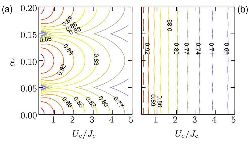
Figure 9: (Color online) Contours of the relative condensate density $\bar{n}_{0}/\bar{n}$ at $T=0$ for (a) $N_{s}=10$ and $\bar{n}=0.5$, and (b) $N_{s}=30$ and $\bar{n}=2$. The values in the plot indicate the relative density of the respective contour.

Next we focus on the interaction Hamiltonian $\hat{H}_{I}$ between BEC and impurities, Eq. (12). As in the continuous case, we only keep terms linear in the fluctuations in the interaction Hamiltonian. Rewriting it in the momentum representation and introducing a macroscopic population of one mode $q_{0}$ yields

$$\begin{split}H_{I}^{(0+1)}&=U_{I}\bar{n}_{0}\sum_{j}\hat{n}_{j}\\ &\quad+\frac{U_{I}\sqrt{N_{0}}}{N_{s}}\sum_{j}\hat{n}_{j}\sideset{}{{}^{\prime}}{\sum}_{q}\Bigl{(}\hat{d}_{q+q_{0}}^{\dagger}\mathrm{e}^{-i2\pi jq/N_{s}}\\ &\qquad+\hat{d}_{q+q_{0}}^{\phantom{\dagger}}\mathrm{e}^{i2\pi jq/N_{s}}\Bigr{)}.\end{split}$$

Here we have shifted the summation index by $q_{0}$ in order for the Bogoliubov transformation, Eq. (22), to be applicable. After application of the transformation we find

$$\begin{split}H_{I}^{(0+1)}&=U_{I}\bar{n}_{0}\sum_{j}\hat{n}_{j}\\ &\quad+\sum_{j}\hat{n}_{j}\sideset{}{{}^{\prime}}{\sum}_{q}\hbar\omega_{q}^{L}\left(M_{j,q}^{L}\hat{b}_{q}^{\phantom{\dagger}}+M_{j,q}^{L*}\hat{b}_{q}^{\dagger}\right),\end{split}$$

where the coupling between the impurities and the Bogoliubov modes is given by

$$M_{j,q}^{L}=\frac{U_{I}\sqrt{N_{0}}}{N_{s}}\frac{1}{\hbar\omega_{q}^{L}}(u_{q}^{*}-v_{q}^{*})\,\mathrm{e}^{-i2\pi jq/N_{s}}.$$

The condensate density $\bar{n}_{0}$ is defined as the macroscopic, condensed part of the total density $\bar{n}=N_{c}/N_{s}$. The noncondensed part then arises from the expectation value of the fluctuation number operators, that is $\bar{n}=\bar{n}_{0}+\sideset{}{{}^{\prime}}{\sum}_{q}\langle\hat{d}_{q}^{\dagger}\hat{d}_{q}^{\phantom{\dagger}}\rangle/N_{s}$. Substituting the fluctuations via Eq. (22) we see that $\bar{n}_{0}$ is implicitly given by

$$\begin{split}\bar{n}&=\bar{n}_{0}+\frac{1}{N_{s}}\sideset{}{{}^{\prime}}{\sum}_{q}\Biggl{[}\frac{\epsilon_{q}^{L}+U_{c}\bar{n}_{0}}{2E_{q}^{L}}\Biggl{(}\frac{2}{\mathrm{e}^{\hbar\omega_{q}^{L}/k_{B}T}-1}+1\Biggr{)}+\frac{1}{2}\Biggr{]}.\end{split}$$

The Boltzmann factor enters through averaging over the phonon distribution at a temperature $T$. In Fig. 9 we plot the relative condensate density $\bar{n}_{0}/\bar{n}$ for two different filling factors and lattice sizes. It becomes clear that our mean field approach is not valid close to the critical values of $\alpha_{c}$ at very low interaction $U_{c}$ because the condensate density vanishes [see Fig. 9(a)]. On the other hand, we see that for small interaction we can assume that $\bar{n}_{0}\simeq\bar{n}$ provided that $\alpha_{c}$ is not too close to a critical value.

References

- Lewenstein et al. (2007) M. Lewenstein, A. Sanpera, V. Ahufinger, B. Damski, A. Sen, and U. Sen, Adv. Phys. 56, 243 (2007), arXiv:cond-mat/0606771.
- Jaksch and Zoller (2005) D. Jaksch and P. Zoller, Ann. Phys. (NY) 315, 52 (2005), arXiv:cond-mat/0410614.
- von Klitzing et al. (1980) K. von Klitzing, G. Dorda, and M. Pepper, Phys. Rev. Lett. 45, 494 (1980).
- Sørensen et al. (2005) A. S. Sørensen, E. Demler, and M. D. Lukin, Phys. Rev. Lett. 94, 086803 (2005), arXiv:cond-mat/0405079.
- Palmer and Jaksch (2006) R. N. Palmer and D. Jaksch, Phys. Rev. Lett. 96, 180407 (2006), arXiv:cond-mat/0604600v1.
- Palmer et al. (2008) R. N. Palmer, A. Klein, and D. Jaksch, Phys. Rev. A 78, 013609 (2008), arXiv:0803.3771v2.
- Schmidt (1997) V. V. Schmidt, The physics of superconductors (Springer, Berlin, 1997).
- Ryu et al. (2007) C. Ryu, M. F. Andersen, P. Clade, V. Natarajan, K. Helmerson, and W. D. Phillips, Phys. Rev. Lett. 99, 260401 (2007), arXiv:0709.0012v2.
- Wilkin and Gunn (2000) N. K. Wilkin and J. M. F. Gunn, Phys. Rev. Lett. 84, 6 (2000), arXiv:cond-mat/9906282v1.
- Cooper et al. (2001) N. R. Cooper, N. K. Wilkin, and J. M. F. Gunn, Phys. Rev. Lett. 87, 120405 (2001), arXiv:cond-mat/0107005v1.
- Schweikhard et al. (2004) V. Schweikhard, I. Coddington, P. Engels, V. P. Mogendorff, and E. A. Cornell, Phys. Rev. Lett. 92, 040404 (2004), arXiv:cond-mat/0308582v2.
- Rosenbusch et al. (2002) P. Rosenbusch, D. S. Petrov, S. Sinha, F. Chevy, V. Bretin, Y. Castin, G. Shlyapnikov, and J. Dalibard, Phys. Rev. Lett. 88, 250403 (2002), arXiv:cond-mat/0201568v2.
- Bretin et al. (2004) V. Bretin, S. Stock, Y. Seurin, and J. Dalibard, Phys. Rev. Lett. 92, 050403 (2004), arXiv:cond-mat/0307464v1.
- Juzeliūnas and Öhberg (2004) G. Juzeliūnas and P. Öhberg, Phys. Rev. Lett. 93, 033602 (2004), arXiv:cond-mat/0402317v2.
- Juzeliūnas et al. (2005) G. Juzeliūnas, P. Öhberg, J. Ruseckas, and A. Klein, Phys. Rev. A 71, 053614 (2005), arXiv:cond-mat/0412015v3.
- Jaksch and Zoller (2003) D. Jaksch and P. Zoller, New J. Phys. 5, 56 (2003), arXiv:quant-ph/0304038v1.
- Klein and Jaksch (2009) A. Klein and D. Jaksch, Europhys. Lett. 85, 13001 (2009), arXiv:0808.1898.
- Morizot et al. (2006) O. Morizot, Y. Colombe, V. Lorent, H. Perrin, and B. M. Garraway, Phys. Rev. A 74, 023617 (2006).
- Gupta et al. (2005) S. Gupta, K. W. Murch, K. L. Moore, T. P. Purdy, and D. M. Stamper-Kurn, Phys. Rev. Lett. 95, 143201 (2005), arXiv:cond-mat/0504749v1.
- Heathcote et al. (2008) W. H. Heathcote, E. Nugent, B. T. Sheard, and C. J. Foot, New J. Phys. 10, 043012 (2008).
- Nandi et al. (2004) G. Nandi, R. Walser, and W. P. Schleich, Phys. Rev. A 69, 063606 (2004).
- Bruderer et al. (2007) M. Bruderer, A. Klein, S. R. Clark, and D. Jaksch, Phys. Rev. A 76, 011605(R) (2007), arXiv:0704.2757v2.
- Bruderer et al. (2008) M. Bruderer, A. Klein, S. R. Clark, and D. Jaksch, New J. Phys. 10, 033015 (2008), arXiv:0710.4493v2.
- Klein et al. (2007) A. Klein, M. Bruderer, S. R. Clark, and D. Jaksch, New J. Phys. 9, 411 (2007), arXiv:0710.3539v2.
- Nunnenkamp et al. (2008) A. Nunnenkamp, A. M. Rey, and K. Burnett, Phys. Rev. A 77, 023622 (2008), arXiv:0711.3831v2.
- Bohigas et al. (1984) O. Bohigas, M. J. Giannoni, and C. Schmit, Phys. Rev. Lett. 52, 1 (1984).
- Kolovsky and Buchleitner (2004) A. R. Kolovsky and A. Buchleitner, Europhys. Lett. 68, 632 (2004), arXiv:cond-mat/0403213v2.
- Mahan (2000) G. D. Mahan, Many-Particle Physics (Kluwer Academic/Plenum Publishers, New York, 2000).
- Buonsante and Wimberger (2008) P. Buonsante and S. Wimberger, Phys. Rev. A 77, 041606(R) (2008), arXiv:0710.1853v3.
- Franke-Arnold et al. (2007) S. Franke-Arnold, J. Leach, M. J. Padgett, V. E. Lembessis, D. Ellinas, A. J. Wright, J. M. Girkin, P. Öhberg, and A. S. Arnold, Opt. Express 15, 8619 (2007).
- LeBlanc and Thywissen (2007) L. J. LeBlanc and J. H. Thywissen, Phys. Rev. A 75, 053612 (2007).
- Petrov et al. (2000) D. S. Petrov, G. V. Shlyapnikov, and J. T. M. Walraven, Phys. Rev. Lett. 85, 3745 (2000), arXiv:cond-mat/0006339v1.
- Castin (2004) Y. Castin, J. Phys. IV France 116, 89 (2004), arXiv:cond-mat/0407118v2.
- Baym et al. (1999) G. Baym, J.-P. Blaizot, M. Holzmann, F. Laloë, and D. Vautherin, Phys. Rev. Lett. 83, 1703 (1999), arXiv:cond-mat/9905430v3.
- Zobay and Rosenkranz (2006) O. Zobay and M. Rosenkranz, Phys. Rev. A 74, 053623 (2006).
- Kohn (1959) W. Kohn, Phys. Rev. 115, 809 (1959).
- Jaksch et al. (1998) D. Jaksch, C. Bruder, J. I. Cirac, C. W. Gardiner, and P. Zoller, Phys. Rev. Lett. 81, 3108 (1998), arXiv:cond-mat/9805329v3.
- Holstein (1959) T. Holstein, Annals of Physics (NY) 8, 343 (1959).
- Madison et al. (2001) K. W. Madison, F. Chevy, V. Bretin, and J. Dalibard, Phys. Rev. Lett. 86, 4443 (2001), arXiv:cond-mat/0101051v1.
- Hodby et al. (2001) E. Hodby, G. Hechenblaikner, S. A. Hopkins, O. M. Marago, and C. J. Foot, Phys. Rev. Lett. 88, 010405 (2001), arXiv:cond-mat/0106262v1.
- Carusotto and Castin (2004) I. Carusotto and Y. Castin, C. R. Physique 5, 107 (2004), arXiv:cond-mat/0311601v2.
- Rey et al. (2007) A. M. Rey, K. Burnett, I. I. Satija, and C. W. Clark, Phys. Rev. A 75, 063616 (2007), arXiv:cond-mat/0611332v1.
- Fetter (1972) A. L. Fetter, Ann. Phys. 70, 67 (1972).
- Ögren and Kavoulakis (2009) M. Ögren and G. Kavoulakis, J. Low Temp. Phys. 154, 30 (2009).
- Landau (1941) L. Landau, J. Phys. U.S.S.R. 5, 71 (1941).
- Leggett (1999) A. J. Leggett, Rev. Mod. Phys. 71, S318 (1999).
- Sykes et al. (2009) A. G. Sykes, M. J. Davis, and D. C. Roberts, Phys. Rev. Lett. 103, 085302 (2009), arXiv:0904.0995.
- Roberts and Pomeau (2005) D. C. Roberts and Y. Pomeau, Phys. Rev. Lett. 95, 145303 (2005).
- Roberts (2006) D. C. Roberts, Phys. Rev. A 74, 013613 (2006).
- Kuper and Whitfield (1963) C. G. Kuper and G. D. Whitfield, eds., Polarons and Excitons (Oliver and Boyd, Edinburgh, 1963).
- Bloch et al. (2008) I. Bloch, J. Dalibard, and W. Zwerger, Rev. Mod. Phys. 80, 885 (2008), arXiv:0704.3011v2.
- Cozzini et al. (2006) M. Cozzini, B. Jackson, and S. Stringari, Phys. Rev. A 73, 013603 (2006), arXiv:cond-mat/0510143v1.
- Nelson et al. (2007) K. D. Nelson, X. Li, and D. S. Weiss, Nat. Phys. 3, 556 (2007).
- van Oosten et al. (2001) D. van Oosten, P. van der Straten, and H. T. C. Stoof, Phys. Rev. A 63, 053601 (2001), arXiv:cond-mat/0011108v1.