Interfacial instability and DNA fork reversal by repair proteins

Abstract

A repair protein like RecG moves the stalled replication fork in the direction from the zipped to the unzipped state of DNA. It is proposed here that a softening of the zipped-unzipped interface at the fork results in the front propagating towards the unzipped side. In this scenario, an ordinary helicase destabilizes the zipped state locally near the interface and the fork propagates towards the zipped side. The softening of the interface can be produced by the aromatic interaction, predicted from crystal structure, between RecG and the nascent broken base pairs at the Y-fork. A numerical analysis of the model also reveals the possibility of a stop and go type motion.

I Introduction

The semi-conservative replication of DNA requires its unzipping by helicases, and synthesis of new strands over the opened parent strands by dna-polymerases (DNA-polymerase III) with high processivitylehn ; baker98 . The basic features of replication are as follows. The two strands of DNA run in opposite directions. The polymerase with unidirectional 3’-5’ motion can then follow the helicase on one strand (the leading strand) only, but not on the other (the lagging strand). Though the two polymerases are identical, the lagging strand polymerase performs a more complicated job, e.g. (i) it makes the new strand in pieces (Okazaki fragments), (ii) it has to shift repeatedly to newer positions closer to the moving helicase, (iii) it restarts the polymerization process anew after every shift, and, then (iv) the small Okazaki fragments are to be joined by dna ligase. In addition primase is required for initiation of the Okazaki fragments, sliding clamp proteins to tether the polymerases to DNA, to name a few more. Moreover, the fidelity of replication requires additional repair or proof-reading capabilities which need to become functional as and when needed. Processivity in this context is defined as the number of base pairs added at a stretch each time the replication machinery binds to DNA (for E. Coli, $4.6\times 10^{6}$ base pair long DNA is ultimately replicated in 40mins). It is understood that most of the polymeric molecules of the replication machinery can work independently in vitro but all of these need to work in tandem over a long time and long distance (along the DNA) for the processivity observed during replication.

The controversy with the replication dynamics can be summarized in the following waylehn ; baker98 . In one class of models, the replication machineries move on the DNA. See Fig. 1a. One needs tight coupling between the lagging strand polymerase and the helicase, though they are independent, to facilitate repeated recognition of the newly unzipped region of DNA. Not only the polymerase and helicase, others like the primase, ligase also need to get correlated on the lagging strand. The antithesis is the proposal of a replisome - a complex of all the objects staying together with the DNA looping through the complex in a very particular mannerodonnell . See Fig. 1b. Since the DNA goes through the replisome, there is expected to be a depletion layer of nutrients surrounding a replisome and it needs to be supplemented by a current towards it. More perplexing is that, if a complex can exist for a long enough time during replication, then why it is so elusive in vitro and what is responsible for the “bound state” in vivo.

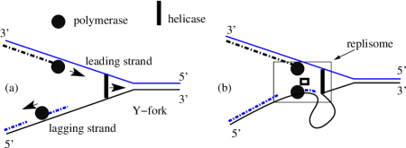
Figure 1: Schematic diagram of the replication process. Only the helicase and the polymerases are shown with arrows indicating directions of motion. The solid lines are the parent DNA strands with 3’, 5’ ends marked. The dash-dot lines represent the newly synthesized DNA. In (a), the members of the replication machinery move on the DNA individually. The small fragments on the lagging strand are the Okazaki fragments. The replisome model is shown in (b). The small thick lined box is the clamp loader that loads the lagging strand DNA on the replisome. In both models, the whole machinery works near the Y-fork.

Single molecular experiments have revealed correlations between synthesis by T7 DNA polymerase and T7 helicase activity on a dsDNA, e.g. efficient duplex DNA synthesis require combined action of polymerase and helicase but no direct or specific interaction between the polymerase and helicase play any rolepatel . For bacteriophage T4, the assembly of the polymerase and the clamp-loader with DNA has been found to be highly dynamic and well coordinatedbenko . The “replisome” may itself be dynamic in nature with not just two but even three polymerases, and others like repair factors can be dynamically attached to itlovett . In case the replication process were tightly controlled, hard-coded in the functioning of the molecules, then that would be reflected in the statistics of the lengths of the Okazaki fragments on the lagging strand as well. The probability distribution of the lengths of these fragments for T4 and T7 have been found to be very broad and highly non-gaussian, compared to very sharp distributions expected from individual primase controlled modelsokazaki . Purely stochastic models have been proposed to study correlations in Okazaki fragment distributionscowan . These newer experimental methods and analysis, apart from elucidating the nature of the complexity of replication, are also bringing out the importance of dynamics and correlations (also called coordination) of the protein complexes and DNA strands in particular near the fork.

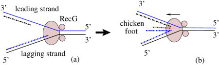
Figure 2: Schematic diagram of the repair process by RecG (shaded ellipse and two circles) at the Y-fork. (a) RecG at the stalled Y-fork with a longer lagging strand pair. (b) Fork reversal and chicken-foot configuration (Holliday junction). The arrow denotes the direction of motion of the fork. The four arm junction is created by the fork reversal and the continuation of the leading strand pair by making use of the pair on the lagging strand.

An important aspect of the replication process is the repair mechanism also involving helicases. A helicase is a motor protein that generally facilitates in opening the DNA and leads the replication machineries. Such a helicase moves from the unzipped (i.e., the open side) to the closed side. There are actually many helicases, e.g. almost 20 in E. Coli (though not clear why so many), but they generically are known to have a part (called the wedge domain) that maintains the two strands of the DNA at a distance much larger than the base pair distance. The motor action (e.g. for dnaBdnab ) and often additional pulling action (e.g. PcrApcra ) carry the opening process on. It stops in case there is a nick or a lesion on the leading strand. The replication process stalls, the whole replication assembly disperses, and a repair process takes over. Often, RecG is the helicase that starts the repair job by performing a fork reversalatkin . Based on the crystal structure, it was suggested that the wedge domain maintains the separation but in addition there are two domains that sit on the zipped side and pushes the DNA towards the unzipped side thereby scooping out the DNA on the lagging strandrecg . See Fig. 2. This continues until the nascent end on the leading strand is reached, forming a chickenfoot configuration. The job of RecG is over, the repair process is completed by other objects via a Holliday junction and then the replication restarts. In this model, RecG has two jobs, zipping the parent strands and unzipping the nascent duplex on the lagging strand. The activities of a pre-assembled RecG-DNA on (i) a three way DNA (consisting of the Y-fork with a nascent duplex on the lagging strand) and (ii) a two-way DNA (consisting of a pure Y-fork) are found to be the same, if initial transients are ignoredmartinez .

We therefore take this view that the main job in the repair process of RecG is the zipping of the DNA or the fork reversal.

Our purpose in this paper is to show how a coupling of the helicase and the replication fork (Y-fork) can be used to formulate the backward mobility of RecG-like repair proteins, in addition to the forward motion of general helicases. Our hypothesis is that the Y-fork is an essential element in the whole replication process, and it is at the heart of the correlated dynamicsepl04 . This hypothesis is based on the observation that in both the biological models and experiments mentioned earlier, the common feature is the proximity of a Y-fork - the junction of an unzipped and a zipped DNA, and dynamics plays an important role, may even be responsible for the formation of the replisome.

The first step to motivate this connection is to analyze the helicase activity. Traditionally, DNA opening is considered a melting phenomenon where thermal noise, fluctuations in base pair breaking-joining, and polymer configurations play important roleslehn . A different mechanism is the force induced unzipping transition at temperatures below the melting pointsmb ; maren ; maren2 ; zip . In the unzipping scenario, a coexistence of the two phases separated by a domain wall, at this first-order transition, is the Y-fork. The wedge domain of a helicase provides the constraint to maintain the DNA in a fixed distance ensemble, and, therefore, a Y-fork develops. The helicase activity is then tantamount to setting the Y-fork interface in motion. In this language, the replication problem can be recast as a velocity selection problem. The Y-fork dynamics is described by the internal dynamics of DNA, the helicase motion is controlled by the energy supply and its own dynamical mechanism, and similarly for other individuals. Thus, each has its own characteristic velocity acting alone, and that’s the velocity one measures in vitrorecbcd . Despite this diversity, these should have the same velocity when together during replication. Hence, the issue of velocity selection. Similarly, a repair process is not just a resealing of the Y-fork under DNA dynamics but has to be closely knit with the repair process. The specialty of RecG comes from the crystal structure which indicates a competition of the closed rings of the wedge domain with the nascent broken pairs of the DNA through aromatic interactionrecg ; atkin . That both the forward and the backward motions can be handled in the same framework lends credence to the basic hypothesis.

The outline of the paper is as follows. Using a Landau type functional to describe the zipped-unzipped coexistence we formulate the propagating front equation when there is a local perturbation around the interface. The coupling of RecG with the interface is then introduced and the effective dynamics written down. This strong coupling that can lead to the elastic or diffusive term to change sign, stabilized by a fourth derivative term, is then studied. This formulation is done in Sec II. A perturbative approach is used to calculate, via a Goldstone mode, the velocity of propagation, the starting point being the zero velocity coexisting phase situation.This is done in Sec III. A numerically exact solution of a discretized version of the model is then presented in Sec IV. Apart from verification of the predictions of the perturbation theory, nonperturbative effects are also found. Sec V is the summary and conclusion.

II Model and velocity selection

II.1 Dynamics

We start with the fact that a double-stranded DNA in equilibrium below its melting point can show phase coexistence with an interface separating the two phases, the zipped and the unzipped phases. A helicase (or its wedge domain mentioned in Sec I) provides the necessary constraint of a fixed distance ensemble to generate the coexistence. To open the DNA this interface needs to be translocated.

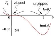
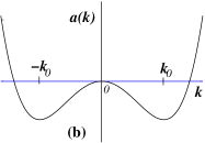
Figure 3: (a) $F_{h}(\phi)$ vs $\phi$ for $h=0$ and $h=0.4$. The perturbation by $h$ makes the unbound state the stable phase. (b) $a(k)$ vs $k$ for the $D^{\prime}<0$ case. The minima at $k=\pm k_{0}$ suggest that the stable state is not the homogeneous state with $\phi=0$ or $1$, but a different state with a modulating wave-vector $k=k_{0}$.

For standard helicases like dnaB, the motor action just forces through the DNA so that as the location of the constraint of the fixed distance ensemble shifts, the bound state region becomes metastable or unstable with respect to the unzipped state. For helicases like PcrA, there is an additional pull by a hand-like branch on the DNA strand near the Y-fork. This is also an example of an active mechanism to make the state near the Y-fork meta- or unstable but not in the bulk. With this in mind, let us formulate our model in the following way. The equilibrium phase coexistence - Y-fork - by a static helicase, can be described by a Landau like free energy $F_{h}(\phi)$ where $\phi$ is a scaled distance. By choosing $\phi=0$ as the bound state and $\phi=1$ as the open state, with a slightly negative $\phi$ representing an overtight state, we take

$$f_{h}(\phi)\equiv-\frac{dF_{h}(\phi)}{d\phi}=\phi(\phi-\frac{1}{2}+h)(1-\phi),$$ (1)

- so that the effective Landau-Hamiltonian can be written as

$${\cal{F}}\{\phi\}=\int dz\left[\frac{D}{2}\left(\frac{\partial\phi}{\partial z}\right)^{2}+F_{h}(\phi)\right],$$ (2)

where $D$ is an elastic constant and

$$F_{h}(\phi)=\frac{\phi^{2}}{4}-\frac{\phi^{3}}{2}+\frac{\phi^{4}}{4}+h\left(-\frac{\phi^{2}}{2}+\frac{\phi^{3}}{3}\right).$$ (3)

The phase coexistence occurs at $h=0$. The coefficients are chosen, for simplicity, to have the extrema of $F_{h}$ in a symmetrical fashion. The perturbation $h>0$ makes the unzipped state the favoured phase. See Fig. 3a. The dynamics is described by

$$\frac{\partial\phi}{\partial t}=\frac{\delta{\cal{F}}}{\delta\phi}=D\frac{\partial^{2}\phi}{\partial z^{2}}+f_{h}(\phi),$$ (4)

with the boundary condition:

$$\phi(-\infty)=1,\ \phi(+\infty)=0,$$ (5)

and $h(z,t)$ is non-zero only near the interface. In Eqs. 1 and 4, $f_{h}$, represents the effective force. The boundary conditions ensure that we have open or unzipped strand on the left side while a closed terminal on the right side. The chain-length has been taken to be infinity. Despite the resemblance, this is not the Fisher-Kolmogorov problemkpp ; wim because there is no bulk instability here.

Where is the helicase in this set of equations? For a static case, $h=0$, and there is no propagation. The boundary conditions impose a kink $\phi(z)$ that goes from $\phi=1$ to $\phi=0$, but the location $z_{0}$ of the kink is arbitrarychaikin . This is a Goldstone-like mode; the interface or the kink separating the unzipped and the zipped phases can be placed anywhere along the chain because neither Eq. 4 cares about $z_{0}$, nor there is any energy cost in shifting the interface. However, a static helicase fixes the position of the Y-fork and therefore it kills the Goldstone mode by fixing $z_{0}$ where the Y-fork would be. The local instability is taken into account by $h(z,t)$ which parametrizes the motor action and the active mechanism of the helicase. In short, the helicase at time $t=0$ is replaced by two features: (i) the time independent boundary conditions and the location of the initial Y-fork represent the wedge domain, and (ii) the passive or active process of the helicase is represented by the local instability parameter $h$.

The dynamic activity of a helicase makes $z_{0}$ a function of time. A propagating mode would imply

$$\phi(z,t)\equiv\Phi(z-ct),$$ (6)

with $c$ the velocity of the front. The helicase must move with the same velocity and the perturbation too, so that

$$h(z,t)\equiv H((z-ct)/W),\ H(z)\neq 0{\ {\rm for}\ }|z|<1.$$ (7)

This matching of velocity is the velocity selection mentioned earlier. $W$ is the width of the region over which the helicase affects the fork. A simpler, more practical, choice would be an implicit definition $h\neq 0$ for $|\phi-\phi_{h}|\leq\delta\phi_{w}$.

RecG is similar to other helicases so far as the existence of a wedge domain is concerned, but its interaction is with the broken bonds at the interface (more like a surfactant). In other words, unlike the ordinary helicases that unzips, it does not produce any instability of any phase but rather interacts with the interface. With that in mind we introduce a new Gaussian variable $y(z,t)$ representing the helicase and its interaction with the interface (for which $\partial\phi/\partial z\neq 0$) as

$${\cal{F}}\{\phi\}=\int dz\left[\frac{D}{2}\left(\frac{\partial\phi}{\partial z}\right)^{2}+F_{0}(\phi)+2\lambda\,y\,\frac{\partial\phi}{\partial z}+Ky^{2}\right],$$ (8)

with $(K>0)$, where the subscript $0$ indicates $h=0$ in Eq. 1, i.e., there is no perturbation in the coexisting part of the free energy.

Instead of coupled dynamics, we consider the effective dynamics of the Y-fork by integrating out the $y$ field. Such an integration leads to a new effective Hamiltonian of the type Eq. 2, with a reduced elastic constant $D^{\prime}=D-\lambda^{2}/K$. For sufficiently large $\lambda$, $D^{\prime}$ can become negative and for stability a higher order term is added. The effective Landau energy can then be taken as

$${\cal{F}}\{\phi\}=\int dz\left[\frac{D^{\prime}}{2}\left(\frac{\partial\phi}{\partial z}\right)^{2}+\frac{\gamma}{2}\left(\frac{\partial^{2}\phi}{\partial z^{2}}\right)^{2}+F_{0}(\phi)\right].$$ (9)

The dynamics is given by

$$\frac{\partial\phi}{\partial t}=D\frac{\partial^{2}\phi}{\partial z^{2}}-\gamma\frac{\partial^{4}\phi}{\partial z^{4}}-h_{R}\frac{\partial^{2}\phi}{\partial z^{2}}+\phi(\phi-\frac{1}{2})(1-\phi),$$ (10)

where the helicase (perturbing) part is written explicitly as the $h_{R}$ term with $h_{R}\neq 0$ in a region near $\phi=0$. We use the fact that RecG operates near the zipped side. With negative $D^{\prime}$, there is a preference for a modulated structure. To see the effect of $D^{\prime}<0$, we rewrite the gradient-dependent part of ${\cal F}\{\phi\}$ in Fourier modes as

$${\cal F}(\phi)=\frac{1}{2}\int\>dk\>a(k)\>\phi_{k}\phi_{-k},$$ (11)

where

$$\phi(z)=\int\frac{dk}{(2\pi)^{1/2}}e^{ikz}\>\phi_{k},\ {\rm and}\ a(k)=D^{\prime}k^{2}+\gamma k^{4}.$$

This favours, as shown in Fig. 3b, a modulated state with wave-vector $k_{0}=\gamma/|D^{\prime}|$. Such a modulated structure would be a state with bubbles - but that does not happen here because the perturbation is only local, meant to destabilize the interface.

The difference between the two types of helicases is now seen in the respective $h$-type terms. In Eq. 4, the $h$-term affects the stability of the phase while in Eq. 10 it affects the interface.

III Perturbative approach

We now treat the helicase effect as a small perturbation and show the change in the direction of velocity in the two cases in a first order perturbation theory. Let us take Eq. 2 for illustration. If there is no perturbation, then the free-energy, Eqs. (1, 2), suggest a static interface, i.e., velocity $c=0$. The profile with small perturbation can therefore be written as

$$\phi=\phi_{0}(z)+\delta\phi(z-ct,t)$$ (12)

where the zeroth order solution is the static solution satisfying

$$D\frac{\partial^{2}\phi_{0}}{\partial z^{2}}+\phi_{0}(\phi_{0}-\frac{1}{2})(1-\phi_{0})=0.$$ (13)

For the boundary conditions of Eq. 4, Eq. 13 gives the static kink solution $\phi_{0}(z)$ that gives the $z$-dependent profile near the interfacechaikin . The perturbed part satisfies to first order an inhomogeneous differential equation

$$\left[\frac{\partial\ }{\partial t}-D\frac{\partial^{2}\ }{\partial z^{2}}-f^{\prime}(\phi_{0})\right]\delta\phi=\delta f(\phi_{0})=h\phi_{0}(1-\phi_{0})$$ (14)

where $f^{\prime}(\phi_{0})=df/d\phi|_{\phi=\phi_{0}}$. This solution of this equation can be written in terms of the Green functionwim

$$\delta\phi=\int_{t_{0}}^{t}d\tau\int_{-\infty}^{\infty}d\xi\>G(t,\tau,z,\xi)\ \delta f(\phi_{0})$$ (15)

Moreover, at first order, the velocity $c$ is small and the perturbed part can be written as

$$\delta\phi=\frac{d\phi_{0}}{dz}\ (t-t_{0})c.$$

This shows that the velocity can be determined from the coefficient of the term linear in $t$.

The Green function has an eigen-function expansion for the spatial part

$$\left[D\frac{\partial^{2}\ }{\partial z^{2}}+f^{\prime}(\phi_{0})\right]\psi_{n}=E_{n}\psi_{n},$$ (16)

where $E_{n}$ are the eigen-values and $\psi_{n}$ the corresponding eigenfunctions. Since we are considering a dissipative system, it is guaranteed that $E_{n}\geq 0$. For all the eigen-functions with $E_{n}>0$, the Green function will have a time contribution $G(t,t_{1},z,z_{1})\sim\exp(-E_{n}(t-t_{1}))$ so that in the long time limit, these modes will not contribute, except for the initial transients.

The Goldstone mode corresponds to a solution with $E_{0}=0$ as can be verified directly with $\psi_{0}=d\phi_{0}/dz$. This zero mode produces the linear term in the solution (not an exponential decay in time) and the velocity of the front comes from this term only. The velocity then is given by

$$c=\frac{\int\phi_{0}^{\prime}(z_{1})(\delta f(z_{1}))dz_{1}}{\int[\phi_{0}^{\prime}(z_{1})]^{2}dz_{1}}.$$ (17)

If the helicase perturbation is operational in a region between $\phi=\phi_{+}$ to $\phi=\phi_{-}$, then the velocity can be written as

$$c=D\frac{\Delta F}{{\cal E}},$$ (18)

where ${\cal E}=\int[\phi_{0}^{\prime}(z)]^{2}dz$ is the kink energy and

$$\Delta F=\int_{\phi_{-}}^{\phi_{+}}\delta f(\phi)d\phi$$

is the free energy cost per unit length in the region of the bite. The expression for the kink energy follows from Eqs. (13) and (8). The velocity found in Eq. 18 is positive, as it should be.

This procedure can be implemented for the RecG case, Eq. 10. The instability of the interface now leads to a moving front but with a negative velocity at least in the perturbative regime. The perturbation theory via the Goldstone mode yields

$$c=-h_{R}\frac{1}{{\cal E}}\left(\frac{\partial\phi_{0}}{\partial z}\right)^{2}\Bigg{|}_{-}^{+},$$ (19)

where the limits are the two end points of the bite. What we see is a negative velocity because of the reduction of the elastic constant and the curvature of the profile of the zeroth order interface near $\phi=0$. By symmetry one would get a positive velocity if the perturbation were at $\phi=1$.

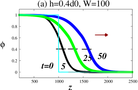
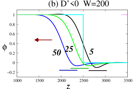
Figure 4: $\phi$ vs. $z$ profile for various times as marked. Both $z$ and $t$ are discretized. (a) For general helicase, Eq. 4 and (b) for RecG-type case for Eq. 10. The horizontal bar indicates the location of the perturbation. In (a) the helicase bites at $\phi=0.5$ while in (b) the bite is at $\phi=0.1$, in both cases over a length $2W$. We see the velocity (direction indicated by an arrow) towards the zipped side in (a) but in the opposite direction in (b). The data are for $D=\gamma=1,h_{R}=2$, so that $D^{\prime}<0$.

III.1 Numerical Solution

The perturbation theory is around the static solution and need not be valid in practical situations. More structures can be expected if we look at the nonperturbative effects of the helicase term in presence of the dynamically generated front. To do so, we solved the discretized versions of the equations numerically via an implicit procedure. The arbitrary lattice spacing $\Delta z$ and time $\Delta t$ are chosen small for convergence. We have taken $\Delta t=10^{-4}$ and $\Delta z=10^{-2}$. All the other parameters are chosen in these units.

The results are shown in Fig. 4 and 5 in discretized $z$ and time $t$. The location $z_{0}$ of the interface is taken to be the point where $\phi=0.5$. We start with a sharp interface at time $t=0$, with $z_{0}$ chosen away from the boundary. Initial transients allow the interface to evolve to its natural shape. This shape in the steady state has been found not to depend on the initial profile. The perturbations are applied over a region as indicated in Fig. 4. For Fig. 4a, the local perturbation favours the unzipped state as shown in Fig. 3a while in Fig. 4b, $h_{R}$ perturbation makes both states unstable (Fig 3b). The velocity measurements were done once the steady state is reached and the interface is not close to the boundaries to avoid finite size or boundary effects.

A check on the perturbation theory would be the linearity of the velocity for small perturbations. We have verified this and also the fact that for a wide perturbation (much larger than the width of the interface) the velocity should saturate to the bulk valueepl04 . These verifications are not shown here. Fig. 4 shows the change in the direction of the velocity by the two perturbations. In (a) the helicase bites at a particular value of $\phi=0.5$, but since the perturbation makes the $\phi=0$ state metastable, the propagation is always towards the zipped side - opening of DNA. In case (b), the bite is also at a particular value of $\phi$ but close to the bound state side. We chose $\phi=0.1$. Owing to the instability of the profile, there is a push towards the unzipped side. The profile in Fig. 4b shows the structure developed - the monotonicity of the profile of Fig. 4a is gone. This non-monotonicity can lead to new phenomenon not captured by the firstorder perturbation. Depending on the width of the bite, there may even be a cancellation in Eq. 19 as we see in the case marked 400 (ignoring the initial transients) In this situation, the helicase would have a stop-and-go type motion, of course towards the unzipped side. Though RecG may not do so, but there are other helicases like RecQ, RecA which are known to have such peculiar motions. Therefore the proposed destabilizing mechanism can lead to varieties of motions. Moreover, these parameters provide us with a set of values to classify or differentiate the helicases quantitatively.

Figure 5: Velocity as a function of time for the RecG type case. because of the continuous change of the profile, the velocity may show a time dependence as seen in the case marked 400 (the spatial width of the perturbation in arbitrary units). Same situation as in Fig. 4b.

IV Summary

A few comments can be made here. In the case of front propagation due to bulk instability, almost a century old problemkpp , there is a pushed to pulled type dynamic transition as reflected in the nature of the velocity of propagationwim . In our approach, the biochemically controllable width $W$ within which a helicase works actually acts as a finite length cut-off for the bulk transition, and, therefore, it provides a new testing ground for any finite size scaling of the bulk nonequilibrium transition. This would be an extremely interesting situation where a biological problem can shed new lights on an age-old physics/material science problem.

Biological models have so far ignored the importance of the interface or treating the Y-fork as a coexistence. We hope our results would motivate new experiments to measure the elastic energy of the interface ($D$), possibly via independent propagation velocity measurement. In addition, the helicases need to be classified by the nature of the perturbation and its strength and width. One needs to wait for these independent experimental results for any quantitative comparisons between the model calculations presented here and related biological experiments.

We summarize our results here. The Y-fork generated by a helicase, if kept in equilibrium, is a coexistence of two phases. Ordinary helicases work by destabilizing the zipped phase near the interface and the local instability leads to the Y-fork motion towards the zipped side, thereby opening the fork. For RecG, the aromatic interaction between the helicase and the interface leads to a destabilization of the interface, and this could close the DNA by a fork motion towards the open side. We show this by a perturbation method that also verifies the results for the ordinary case. A numerically exact solution is used to study the Y-fork motion in presence of the dynamically generated front. In the interface destabilization case, more complex stop-and-go type motion is found to be possible. Coming back to the problem of replication, our results enable us now to use this formulation to describe the replication in a co-moving frame with the Y-fork, bypassing a direct reference to the helicase. It remains to be seen if one can couple the Y-fork motion with the polymerase activity.

References

- (1) A. L. Lehninger, Principles of Biochemistry, 5ed, W.H. Freeman, New York, 2008
- (2) T. A. Baker and S. P. Bell, Cell, 92, 295 (1998).
- (3) M. O’Donnell, J. Bio. Chem., 281 10653 (2006); Nina Y. Yao et al, PNAS 106 13236 (2009).
- (4) D. Fass, C. E. Bogden and J. M. Berger, Structure, 7, 691 (1999).
- (5) N. M. Stano et al, Nature 435 370 (2005).
- (6) M. A. Trakselis, et al, PNAS, 98 8368 (2001).
- (7) S. T. Lovett, Mol. Cell, 27 523 (2007).
- (8) P. D. Chastain II etal, Mol. Cell 6 803 (2000).
- (9) R. Cowan, in Handbook of Statistics, Vol 20, p137, Ed. C. R. Rao and D. N. Shanbang, North-Holland, Amsterdam (2001).
- (10) P. Soultanas et al., EMBO J. 19 3799 (2000).
- (11) J. Atkinson and P. McGlynn, Nucleic Acids Research 37, 3475 (2009).
- (12) M. R. Singleton, S. Scaife,and D. B. Wigley, Cell 107, 79 (2001).
- (13) M. M. Martinez-Senac and M. R. Webb, Biochem. 44 16967 (2005).
- (14) S. M. Bhattacharjee, Europhysics Letts. 65, 574 (2004)
- (15) S. M. Bhattacharjee, J. Phys. A, 33 L423 (2000); (cond-mat/9912297).
- (16) Jeff Z.Y. Chen, Phys. Rev. E 66, 031912 (2002); A. E. Allahverdyan et al., Phys. Rev. E 69, 061908 (2004); Pui-Man Lam, J. C. S. Levy, and Hanchen Huang, Biopolymers 73, 293 (2004); R. Kapri, J. Chem. Phys. 130, 145105 (2009).
- (17) D. Marenduzzo, A. Trovato, and A. Maritan, Phys. Rev. E 64, 031901 (2001).
- (18) R. Kapri, S. M. Bhattacharjee and F. Seno Phys. Rev. Lett. 93, 248102 (2004); R. Kapri, S. M. Bhattacharjee Phys. Rev. Lett. 98, 098101 (2007)
- (19) P. R. Bianco, et al., Nature 409 374 (2001); K. M. Dohoney and J. Gelles, Nature 409, 370 (2001).
- (20) R. Luther, Z. Elektrochem. 12, 596 (1906); R. A. Fisher, Ann. Eugenics. 7, 355 (1937); A. Kolmogorov, L. Petrovsky and N. Piscounoff, Bull. Univ. Moscow, Ser. Int., Sect. A 1,1 (1937).
- (21) Wim van Saarloos, Phys. Rept. 386, 29 (2003).
- (22) P. M. Chaikin and T.C. Lubensky, Principles of Condensed Matter Physics, (Cambridge University Press, Cambridge, 1995).