Linear response theory of activated surface diffusion with interacting adsorbates

Abstract

Activated surface diffusion with interacting adsorbates is analyzed within the Linear Response Theory framework. The so-called interacting single adsorbate model is justified by means of a two-bath model, where one harmonic bath takes into account the interaction with the surface phonons, while the other one describes the surface coverage, this leading to defining a collisional friction. Here, the corresponding theory is applied to simple systems, such as diffusion on flat surfaces and the frustrated translational motion in a harmonic potential. Classical and quantum closed formulas are obtained. Furthermore, a more realistic problem, such as atomic Na diffusion on the corrugated Cu(001) surface, is presented and discussed within the classical context as well as within the framework of Kramer’s theory. Quantum corrections to the classical results are also analyzed and discussed.

I Introduction

The main purpose of spectroscopic experiments involving a probe and a system at thermal equilibrium with a reservoir or thermal bath consists of measuring the system response under the perturbation caused by the probe gordon ; mcquarrie . The intrinsic properties of matter can be extracted by analyzing this response, which thus becomes a very important tool for physicists, who can elucidate the microscopic structure and its dynamics through it. Many times this response can be described by first order perturbation theory and determined by the spectrum of the spontaneous fluctuations of the reservoir, as established by the so-called fluctuation-dissipation (FD) theorem kubo . Within this linear approximation, the probability per time unit that the full system formed by probe and reservoir changes from the initial state to the final state is given by the Fermi golden rule. More specifically, the probe transition probability from an initial state to a certain final state is given by the time Fourier transform of the autocorrelation function associated with the operator defined by the matrix element of the corresponding interaction Hamiltonian. This type of studies is based on the work developed by van Hove vanhove ; vineyard , who introduced the space-time correlation function (namely the van Hove function), a generalization of the well-known pair-distribution function from the theory of liquids, as a tool to study the scattering of probe particles (slow neutrons) by quantum systems consisting of interacting particles at thermal equilibrium. Within the Born approximation in scattering theory, the nature of the scattered particles as well as the details of the system-probe interaction potential are largely irrelevant, this essentially reducing the scattering problem to a typical statistical mechanics problem lovesey . The linear response function of a system consisting of interacting particles, also known as dynamic structure factor or scattering law, can be then related to the spontaneous-fluctuation spectrum of such particles and expressed in terms of particle density-density correlation functions lovesey ; hansen ; bee . As is known, a complete description of this dynamics can also be obtained through the linear response theory, where the FD theorem is used to derive alternative response function expressions for the dynamic structure factor.

From quasielastic He atom scattering (QHAS) experiments at low energies very detailed information about defect and adsorbate dynamics on surfaces can be obtained lahee ; manson ; hofmann ; eli1 . Manson and Celli manson generalized van Hove’s theory of neutron scattering by crystals and liquids to atom surface scattering within the transition matrix formalism. Within this approach, small coverage of adsorbates and/or defects were assumed in order to ignore both their interactions as well as multiple scattering with He atoms. Diffuse elastic and inelastic features were interpreted again through the dynamical structure factor which is proportional to the observed line shapes and is expressed in terms of the transfer of energy and parallel momentum to the He atoms before and after the scattering process. The QHAS technique has also been applied to study surface diffusion on metals with different types of atomic and molecular adsorbates, the diffusion of Na adatoms (at different coverages) on Cu(001) being one of the most extensively studied systems. In the case of massive particles, where very large timescales are involved, the dynamic structure factor can be expressed in terms of the adsorbate positions, which has led to the so-called single adsorbate model. Within this approach, where low coverage is assumed, surface diffusion (i.e., the adsorbate motion) is described by classical stochastic trajectories of adsorbates issued from solving the standard Langevin equation. As in the case of Brownian-like particles, this equation encompasses two contributions: (1) a (external) force arising from the deterministic, phenomenological adiabatic potential describing the adsorbate-substrate interaction at zero surface temperature; and (2) a stochastic force (usually, a Gaussian white noise) accounting for the vibrational effects induced by the temperature on the surface lattice atoms (and therefore on the adsorbates). The system dynamics is then obtained after solving the Langevin equation graham ; elis ; eli1 ; vega1 ; vega2 , analyzing the results derived from it in terms of the so-called motional narrowing effect vega1 ; vega2 as well as Kramers’ turnover theory vega3 ; guantes1 and the dephasing theory guantes2 . Within this scenario, it is usually assumed that He-adsorbate interactions play no role on the surface dynamics, thus being scarcely analyzed.

When the coverage is increased, the dynamic structure factor also provides valuable information about the nature of the adsorbate-adsorbate interaction, which should be included in the corresponding theoretical studies. In this way, pairwise potential functions accounting for the adsorbate-adsorbate interactions are usually introduced into Langevin molecular dynamics (LMD) simulations elis . Recently, an alternative procedure has been considered, where such pairwise interactions are described by a purely stochastic model, namely the interacting single adsorbate (ISA) model ruth1 ; ruth2 ; ruth3 ; ruth4 . This approach, also within the standard Langevin framework, is based on both the theory of spectral-line collisional broadening developed by van Vleck and Weisskopf vvleck-weiss and the elementary kinetic theory of gases mcquarrie , and explains fairly well the experimental broadening observed with increasing coverage elis . The standard Langevin equation is solved with two different, non-correlated noise functions: (1) a Gaussian white noise accounting for the surface friction, as before, and (2) a white shot noise gardiner replacing the pairwise interaction potential which simulates the adsorbate-adsorbate collisions. A double Markovian assumption is therefore considered (for the interaction with the surface and for the interaction among adsorbates). This assumption holds because, on the one hand, substrate excitation timescales are much shorter than the timescales associated with the adatom motions (the maximum frequency of the substrate excitation is around 20-30 meV, while the characteristic vibrational frequency of the adatom is around 4-6 meV). On the other hand, the time between consecutive collisions (measured through a collisional frequency, which would depend on temperature, coverage or the adparticle mass) is typically much longer than the effective time that a collisional effect may last (i.e., the time two adsorbates may effectively be in physical contact). Therefore, memory effects are not taken into account. Just as the adsorbate-surface interaction is characterized by a (surface) friction, the adsorbate-adsorbate interaction will also be describable in terms of a collisional friction, which will vary with coverage. With this simple stochastic model, where the total friction is the sum of the substrate friction and the collisional friction, a good agreement with the experimental results for coverages up to 0.12, approximately, has been obtained. For higher coverage values, the model cannot be applied due to the appearance of ordered structures, as it has been observed ellis experimentally between 0.12 and 0.16. Recently, the collisional friction has been estimated from experiments with benzene on graphite allison0 . Although further investigation at a microscopic level and first-principle calculations are needed, this simple stochastic model at moderate coverages is able to provide a complementary view of diffusion (through the quasielastic Q-peak) and low frequency vibrational motions (through the frustrated translational T-mode peak), at or around zero energy transfers (very long time dynamical processes), respectively. This could be understood because any trace of the true interaction potential seems to be wiped out due to the relatively large number of collisions taking place at very long times (the time scale for the diffusion regime). Actually, this purely stochastic model can be derived from a microscopic classical Hamiltonian model characterized by two baths associated with two independent collections of harmonic oscillators german , one related to the surface phonons and the other one describing the presence of adsorbates, the source of the collisional friction. In this model, the coupling to low-lying electron-hole excitations (electroninc friction) was not considered for simplicity. One of the purposes in the present work is to extend this two-bath model to quantum activated diffusion.

Surface diffusion processes are also studied experimentally by means of the so-called spin echo techniques. Thus, since the advent of He spin echo (HeSE) spectroscopy allison1 ; allison2 ; allison3 and the improved signal in the neutron spin echo (NSE) spectrometer farago ; fouquet , fast diffusion processes are more accessible and allow us to to better determine interaction potentials. In both types of experiments, the observable is the so-called intermediate scattering function or polarization function, which is the inverse time Fourier transform of the dynamic structure factor. This is a complex function whose real and imaginary parts can be observed experimentally allison2 ; allison3 . The intermediate scattering function is also the space Fourier transform of the van Hove function, which, in general, is also a complex-valued function. The complex character of these functions can be understood as a signature of the quantum nature of the diffusion dynamics. In this regard, a quantum Markovian theory of surface diffusion for interacting adsorbates has also been proposed recently ruth5 . The imaginary part of the van Hove function is important at small values of time or high temperatures (timescales of the order of $\hbar\beta$, with $\beta=1/k_{B}T$, $k_{B}$ being Boltzmann’s constant). This dynamical regime takes place when the mean de Broglie wavelength $\lambda_{B}=\hbar/\sqrt{2mk_{B}T}$ ($m$ is the adsorbate mass) is of the order of or greater than typical interparticle distances. For these timescales and distances, the adparticle positions are no longer variables, but Heisenberg operators that do not commute at two different times. This theory thus tries to reconcile classical and quantum calculations when no diffusion by tunneling is considered.

The purpose of this work is to provide an analysis of activated surface diffusion with interacting adsorbates within the linear response theory framework. The theoretical framework of the aforementioned two-bath model is then applied to simple systems, such as diffusion on flat surfaces and the frustrated translational motion in a harmonic potential, obtaining classical and quantum closed formulas. Moreover, a more realistic problem, such as atomic Na diffusion on on the corrugated Cu(001) surface, is presented and discussed within the classical context as well as within the framework of Kramer’s theory, introducing quantum corrections to the classical results which will be analyzed and discussed. Note that an appropriate understanding of this surface dynamics is very important, for diffusion is a preliminary step in more complicated surface phenomena, such as heterogeneous catalysis, crystal growth, lubrication, associative desorption, etc. Furthermore, the QHAS and HeSE techniques can be considered as the surface science analogue of the quasielastic neutron scattering techniques, which has been widely and successfully applied to analyze diffusion in bulk.

According to our purposes, we have organized this work as follows. In Section II, we give a general overview of the Linear Response Theory applied to activated surface diffusion. In particular, a revision of the classical two-bath model is presented. Regarding the quantum version of this model, a proposal and discussion are also given in order to describe the stochastic trajectories of the adsorbates at different coverages. In Section III, applications to simple models (flat surfaces and driven damped harmonic oscillator) as well as to more realistic problems, as atomic Na diffusion on Cu(001), are analyzed within the context of classical and quantum dynamics. Kramers’s turnover theory is also analyzed within the classical context. Finally, in Section IV we summarize the conclusions derived from this work as well as some future work.

II General theory for activated surface diffusion

II.1 Dynamic structure factor and intermediate scattering function

Space-time correlation functions yip91 can be used to describe the decay of spontaneous thermal fluctuations at surfaces, being central to the study of transport phenomena. These functions are defined as the thermodynamic average of the product of two dynamical variables, each one expressing the instantaneous deviation from its corresponding equilibrium value at particular points on the surface and time. A complete description of the particle dynamics in a many-body system is then reached when the behavior of the corresponding correlation functions over the entire wavenumber range is studied. This range splits into different characteristic regions, each one associated with a different set of properties of the system. In the case of scattering experiments, since the momentum and energy transfers are the relevant quantities, any correlation-function theory has to be developed necessarily in terms of such quantities. Space-time correlation functions can also be used to describe the response of a fluid under a weak, external perturbation. Indeed, the reason why space-time correlation functions are central quantities in transport phenomena in fluids is, precisely, because of the equivalence between spontaneous fluctuation and linear response.

In general, a surface local dynamical variable is defined as

$$A({\bf R},t)=\frac{1}{\sqrt{N}}\sum_{i=1}^{N}a_{i}(t)\delta({\bf R}-{\bf R}_{i}(t)),$$ (1)

where $a_{i}(t)$ is any physical quantity and ${\bf R}_{i}(t)=(x_{i}(t),y_{i}(t))$ is the time-dependent center of the position operator of the adparticle on a two-dimensional surface. The corresponding fluctuation is usually defined as $\delta A({\bf R},t)=A({\bf R},t)-\langle A({\bf R},t)\rangle_{\beta}$, where the average on a canonical ensemble is denoted by $\langle\ \cdot\ \rangle_{\beta}$. The dynamical variable conserves if it satisfies a continuity equation of the form

$$\dot{A}({\bf R},t)=-\nabla_{\bf R}\cdot{\bf J}_{A}({\bf R},t),$$ (2)

where ${\bf J}_{A}$ is the current associated with the $A$ variable and the dot over $A$ denotes the total time derivative. Here, the dynamical variables of particular interest are the number density,

$$\rho({\bf R},t)=\frac{1}{\sqrt{N}}\sum_{i=1}^{N}\delta({\bf R}-{\bf R}_{i}(t)),$$ (3)

and the current density

$${\bf J}({\bf R},t)=\frac{1}{\sqrt{N}}\sum_{i=1}^{N}{\bf v}_{i}(t)\delta({\bf R}-{\bf R}_{i}(t)),$$ (4)

where ${\bf v}_{i}$ accounts for the velocities of the $N$ adparticles. The corresponding van Hove fluctuation density autocorrelation function vanhove ; lovesey reads as

$$G(|{\bf R}-{\bf R}^{\prime}|,t)=\Sigma\langle\delta\rho({\bf R}^{\prime},0)\delta\rho({\bf R},t)\rangle_{\beta},$$ (5)

and a similar expression holds for the current density. The adparticle density is given by $\rho=N/\Sigma$, where $\Sigma$ is the surface area and the coverage is defined by $\theta=N/N_{\rm max}$, with $N_{\rm max}$ being the maximum number of sites in the $\Sigma$ area. In most physical systems, correlation effects are negligible at large space or time separation, the asymptotic limit being a simple product of thermodynamically averaged quantities.

In analogy to scattering of slow neutrons by crystals and liquids vanhove ; vineyard ; lovesey , the observable magnitude in QHAS experiments is the so-called differential reflection coefficient,

$$\frac{d^{2}\mathcal{R}(\Delta{\bf K},\omega)}{d\Omega d\omega}=n_{d}\mathcal{F}S(\Delta{\bf K},\omega).$$ (6)

This coefficient gives the probability that the He atoms (probe particles) scattered from the interacting adsorbates on the surface reach a certain solid angle $\Omega$ with an energy exchange $\hbar\omega=E_{f}-E_{i}$ and wave vector transfer parallel to the surface $\Delta{\bf K}={\bf K}_{f}-{\bf K}_{i}$. In Eq. (6), $n_{d}$ is the concentration of adparticles; ${\mathcal{F}}$ is the atomic form factor, which depends on the interaction potential between the probe atoms in the beam and the adparticles on the surface; and $S(\Delta{\bf K},\omega)$ is the dynamic structure factor, which gives, apart from other peaks, the Q and T-mode peaks, also providing a complete information about the dynamics and structure of the adsorbates through particle distribution functions. Experimental information about long distance correlations is obtained from the dynamic structure factor when considering small values of $\Delta{\bf K}$, while information on long time correlations is provided at small energy transfers, $\hbar\omega$.

The pair distribution functions are given by means of the van Hove or time-dependent pair correlation function $G({\bf R},t)$ vanhove . This function is related to the dynamic structure factor by a double Fourier transform, in space and time, as

$$S(\Delta{\bf K},\omega)=\frac{1}{2\pi\hbar N}\int\!\!\!\int G({\bf R},t)e^{i(\Delta{\bf K}\cdot{\bf R}-\omega t)}\ \!d{\bf R}\ \!dt.$$ (7)

Given an adparticle at the origin at some arbitrary initial time, $G({\bf R},t)$ represents the average probability to find a particle (the same or another one) at the surface position ${\bf R}=(x,y)$ at a time $t$. Thus, this function generalizes the well–known pair distribution function $g({\bf R})$ from statistical mechanics mcquarrie ; hansen by providing information about the interacting particle dynamics.

The position operators of the adsorbates are given, in general, by the corresponding Heisenberg operators (defined for all $j=1,\cdots,N$ adparticles and time $t$),

$${\bf R}_{j}(t)=e^{iHt/\hbar}{\bf R}_{j}e^{-iHt/\hbar},$$ (8)

where $H$ is the Hamiltonian of the total system. As mentioned above, the space Fourier transform of the $G$-function is the intermediate scattering function,

$$I(\Delta{\bf K},t) = N\int\!\!\!\int G({\bf R},t)e^{i\Delta{\bf K}\cdot{\bf R}}\ \!d{\bf R}$$ (9)

$$= \frac{1}{N}\langle\rho_{\Delta{\bf K}}(t)\rho^{\dagger}_{\Delta{\bf K}}(0)\rangle_{\beta},$$

where the $\rho_{\Delta{\bf K}}$ operator defined as

$$\rho_{\Delta{\bf K}}(t)=\sum_{j=1}^{N}e^{-i{\Delta{\bf K}}\cdot{\bf R}_{j}(t)}=\rho^{\dagger}_{-\Delta{\bf K}}(t)$$ (10)

is the Fourier component of the adsorbate number-density operator,

$$\rho({\bf R},t)=\sum_{j=1}^{N}\delta({\bf R}-{\bf R}_{j}(t)).$$ (11)

Thus, in (9) the brackets denote the ensemble average over the trajectories associated with each adsorbate ${\bf R}_{j}(t)$. The intermediate scattering function is the typical observable issued from HeSE and NSE experimental techniques. Taking into account the relations (7) to (11), we note that the dynamic structure factor can be expressed in terms of a density-density correlation function and determined by the spectrum of the spontaneous fluctuations. Moreover, the static structure factor, defined as $S(\Delta{\bf K},t=0)$, is related to $g({\bf R})$, which describes the instantaneous correlation between adsorbates.

From relations (3) and (4), one finds by direct differentiation in the reciprocal space the continuity or number conservation equation,

$$\frac{\partial\rho_{\Delta{\bf K}}(t)}{\partial t}=i\Delta{\bf K}\cdot{\bf J}_{\Delta{\bf K}}(t),$$ (12)

which inserted into (9), and taking into account (7), we obtain the basic relation

$$S(\Delta{\bf K},\omega)=\frac{\Delta{\bf K}^{2}}{\omega^{2}}J_{l}(\Delta{\bf K},\omega),$$ (13)

where $J_{l}$ is the longitudinal (projected along the wave vector transfer direction) current correlation function. This relation is rigorous as far as the adparticles are not being created or absorbed.

The dynamic structure factor $S(\Delta{\bf K},\omega)$ is an even function in frequency. Therefore, all the odd moments vanish and the frequency moments or frequency sum rules (static correlation functions) are $\Delta{\bf K}$-dependent quantities,

$$\omega^{2n}(\Delta{\bf K})=\frac{1}{2\pi}\int\omega^{2n}S(\Delta{\bf K},\omega)d\omega=(-1)^{n}\left[\frac{\partial^{2n}I(\Delta{\bf K},t)}{\partial t^{2n}}\right]_{t=0},$$ (14)

which are obtained from a Taylor series expansion of the intermediate scattering function at short times (or small distances). In particular, the zeroth-order moment corresponds to the static structure factor,

$$\omega^{0}(\Delta{\bf K})=S(\Delta{\bf K}),$$ (15)

since it describes the average distribution of interparticle distances on the surface; the second order moment is related to the thermal speed $v_{0}=\sqrt{2k_{B}T/m}$, as

$$\omega^{2}(\Delta{\bf K})=\Delta{\bf K}^{2}v_{0}^{2}.$$ (16)

Due to the quantum character of the different operators introduced above, several comments are worth stressing. First, $\rho_{\Delta{\bf K}}(t)$ and $\rho_{\Delta{\bf K}}^{\dagger}(0)$ commute only at $t=0$. Second, the system studied here is assumed to be stationary and, therefore, the origin of time is arbitrary for the correlation function associated with the density operators. Third, the complex character of the corresponding correlation function is a signature of the quantum dynamics of the interacting system. Fourth, the $G$-function is also complex, but the dynamic structure factor is real and positive definite because it represents a cross-section. More properties of the $\rho_{\Delta{\bf K}}(t)$ operator, the $G$-function and the dynamic structure factor can be found in Lovesey’s book lovesey . And fifth, the so-called detailed balance condition can be expressed as schofield

$$S(\Delta{\bf K},\omega)=e^{\hbar\omega\beta}S(-\Delta{\bf K},-\omega),$$ (17)

which expresses that the probability that a He atom loses an energy $\hbar\omega$ is equal to $e^{\hbar\omega\beta}$ times the probability that a He atom gains an energy $\hbar\omega$.

After van Hove vanhove , if $R_{0}$ is the range of the $G$-function and $T_{0}$ its relaxation time, $\hbar/R_{0}$ and $\hbar/T_{0}$ determine the orders of magnitude of average momentum and energy transfers in the scattering process of the probe particles, which for light masses display the observable recoil effect. Thus, the time variation of $G$ affects the total scattering and angular distributions only for a particle spending at least a time of order $T_{0}$ over a correlation length $R_{0}$. Moreover, if the mean de Broglie wavelength, $\lambda_{B}$, is small compared to interadparticle distances or the range of adsorbate-adsorbate interaction, no quantum effect will manifest in the $G$-function, which deals with pairs of adparticles separated by distances of the order of $R_{0}$. Nevertheless, for small timescales ($t\ll T_{0}$ or $t\sim\hbar\beta)$), the dynamics entirely concentrates in a region of the order of or less than $\lambda_{B}$, and quantum effects are noticeable. At these distances, the adparticles can be considered as a two-dimensional free gas. The imaginary part of the $G$-function is greater at small values of time.

II.2 The Hamiltonian for the system and the thermal bath

II.2.1 The one-bath model

In order to go a step further into the dynamics, we need to specify a Hamiltonian as introduced in Eq. (8). In surface diffusion, the full system+bath Hamiltonian is usually written eli1 as

$$H = \frac{p_{x}^{2}}{2m}+\frac{p_{y}^{2}}{2m}+V(x,y)$$ (18)

$$+\sum_{i=1}^{N}\left[\frac{p_{x_{i}}^{2}}{2m_{i}}+\frac{m_{i}}{2}\left(\omega_{x_{i}}x_{i}-\frac{c_{x_{i}}}{m_{i}\omega_{x_{i}}}\ \!x\right)^{2}\right]$$

$$+\sum_{i=1}^{N}\left[\frac{p_{y_{i}}^{2}}{2m_{i}}+\frac{m_{i}}{2}\left(\omega_{y_{i}}y_{i}-\frac{c_{y_{i}}}{m_{i}\omega_{y_{i}}}\ \!y\right)^{2}\right],$$

where $(p_{x},p_{y})$ and $(x,y)$ are the adparticle momenta and positions, and $(p_{x_{i}},x_{i})$ and $(p_{y_{i}},y_{i})$ with $i=1,\cdots,N$ are the momenta and positions of the bath oscillators (phonons), with mass and frequency given by $m_{i}$ and $\omega_{i}$, respectively; phonons with polarization along the $z$-direction are not considered. The Hamiltonian was originally considered by Magalinskii maga and Caldeira and Leggett caldeira , who used it for weak and strong dissipation (a general discussion about the Hamiltonian (18) can be found in Weiss’ book weiss ). In surface diffusion, $V(x,y)$ is in general a periodic function describing the surface corrugation at zero temperature.

The harmonic frequencies of the bath modes and the coupling coefficients are expressed in terms of spectral densities, defined caldeira as

$$J_{i}(\omega)=\frac{\pi}{2}\sum_{j=1}^{N}\frac{c_{i_{j}}^{2}}{m_{j}\omega_{i_{j}}^{2}}\left[\delta(\omega-\omega_{i_{j}})\right].$$ (19)

with $i=x,y$. This enables the passage to a continuum model. The associated friction functions are defined through the cosine Fourier transform of the spectral densities as

$$\eta_{i}(t)=\frac{2}{\pi m}\int_{0}^{\infty}d\omega\frac{J_{i}(\omega)}{\omega}\cos\omega t,$$ (20)

with $i=x,y$. For Ohmic friction, $\eta_{i}(t)=2\eta_{i}\delta(t)$ where $\eta_{i}$ is a constant and $\delta(t)$ is the Dirac delta function. In this model, the noise is shown to be white when Ohmic friction is assumed. The paradigm of white noise is the Gaussian white noise. Dealing with large systems (the surface seen as a thermal bath) where the number of collisions between substrate and adsorbate is very high, the fundamental theorem of probability theory, namely the central limit theorem, assures that the fluctuations of the bath will be Gaussian distributed. Diffusion can then be described by a Brownian-type motion involving a continuous Gaussian stochastic process. In virtue of the FD theorem, such fluctuations can be related to the friction coming mainly from surface phonons: the phonon friction. Electronic friction due to low-lying electron-hole pair excitations are usually neglected in most of cases.

II.2.2 The two-bath model

The diffuse elastic intensity of the He atoms scattered at large angles away from the specular direction provides very detailed information on the mobility of adsorbates on surfaces. Based on the transition matrix formalism, Manson and Celli manson proposed a quantum diffuse inelastic theory for small and intermediate coverages of adsorbates on the surface by ignoring multiple scattering effects of He atoms. The dynamical structure factor is then obtained by assuming all the crystal vibrational modes ($N$) and point-like scattering centers ($M$) satisfying the harmonic approximation with a given frequency distribution function. Therefore, following the same type of arguments, we could assume two independent, uncorrelated baths to describe diffusion of interacting adsorbates. As before, the first bath consists of the surface phonons. Meanwhile, the second bath is formed by $M$ adsorbates which, obviously, changes with the surface coverage given by experimental conditions german .

For a two-bath model (for a given coverage), we take one adsorbate as the tagged particle or system, while the remaining ones constitute the second bath descibed by $M$ harmonic oscillators. In this way, the corresponding total Hamiltonian reads as german

$$H = \frac{p_{x}^{2}}{2m}+\frac{p_{y}^{2}}{2m}+V(x,y)$$ (21)

$$+\sum_{i=1}^{N}\left[\frac{p_{x_{i}}^{2}}{2m_{i}}+\frac{m_{i}}{2}\left(\omega_{x_{i}}x_{i}-\frac{c_{x_{i}}}{m_{i}\omega_{x_{i}}}\ \!x\right)^{2}\right]$$

$$+\sum_{i=1}^{N}\left[\frac{p_{y_{i}}^{2}}{2m_{i}}+\frac{m_{i}}{2}\left(\omega_{y_{i}}y_{i}-\frac{c_{y_{i}}}{m_{i}\omega_{y_{i}}}\ \!y\right)^{2}\right]$$

$$+\sum_{j=1}^{M}\left[\frac{{\bar{p}}_{x_{j}}^{2}}{2{\bar{m}}_{j}}+\frac{{\bar{m}}_{j}}{2}\left({\bar{\omega}}_{x_{j}}{\bar{x}}_{j}-\frac{d_{x_{j}}}{{\bar{m}}_{j}{\bar{\omega}}_{x_{j}}}\ \!x\right)^{2}\right]$$

$$+\sum_{j=1}^{M}\left[\frac{{\bar{p}}_{y_{j}}^{2}}{2{\bar{m}}_{j}}+\frac{{\bar{m}}_{j}}{2}\left({\bar{\omega}}_{y_{j}}{\bar{y}}_{j}-\frac{d_{y_{j}}}{{\bar{m}}_{j}{\bar{\omega}}_{y_{j}}}\ \!y\right)^{2}\right],$$

where the barred magnitudes label the same quantities as in the one-bath model, but now referring to a bath of $M$ adsorbates, which are also considered as a collection of harmonic oscillators. The $c_{k_{j}}$ and $d_{k_{j}}$ coefficients, with $k=x,y$, give the coupling strengths between the adsorbate and the substrate phonons or other adsorbates, respectively. The spectral density for the two baths is defined analogously to the one-bath model,

$$J_{i}(\omega)=\frac{\pi}{2}\sum_{j=1}^{N}\frac{c_{i_{j}}^{2}}{m_{j}\omega_{i_{j}}^{2}}\left[\delta(\omega-\omega_{i_{j}})\right]+\frac{\pi}{2}\sum_{j=1}^{M}\frac{d_{i_{j}}^{2}}{{\bar{m}}_{j}{\bar{\omega}}_{i_{j}}^{2}}\left[\delta(\omega-{\bar{\omega}}_{i_{j}})\right],$$ (22)

but now it is split into two sums, one spectral density due to the surface phonons and the other one due to adsorbates. In a similar way, the friction functions are defined as in Eq. (20) but now the spectral density is given by (22). The friction function is also split into two terms, one due to the phonons, $\gamma(t)$, and the other one due to the presence of adsorbates, $\lambda(t)$. This last friction function could be interpreted like a collisional friction. Again, for Ohmic friction, $\eta_{i}(t)=2(\gamma+\lambda)\delta(t)$, where $\gamma$ and $\lambda$ are constant and $\delta(t)$ is the Dirac delta function.

Extension of the one-bath model to two baths is carried out to describe collisions among adsorbates when the coverage is increased up to a certain value. Again, if the friction is assumed to be Ohmic, the noise will be white. Adsorbate collisions can be seen as discrete events. It is well known that an appropriate way to model this type of noise is by considering a Poisson process, being generally designated as a white shot noise. As has been shown elsewhere ruth2 ; ruth3 , this white shot noise can be obtained as a limiting case of a color noise. It is also clear that when the diffusion regime is reached, the discrete Poisson process becomes a continuous Gaussian process. The introduction of the second bath allows us to describe adsorbate collisions by a new friction coefficient, the collisional friction. If the two baths are not correlated, the corresponding noises are also not correlated and this is the key point of the ISA model. The total friction coefficient, the sum of the phonon and collisional frictions, is related to the fluctuations of both baths through the FD theorem. This sum of frictions has recently been estimated by the He spin echo technique allison0 ; allison3 .

Before concluding this subsection, we would like to emphasize that if an external driving force is also present (He atoms are sampling the surface to explore the motion of adparticles) a new extra term should be added to the total Hamiltonian, (18) or (21) (see Section III).

II.3 The Langevin equation in the two-bath model

The next task is to eliminate the environmental (two-baths) degrees of freedom, which leads to a damped equation of motion of the system coordinates. If the Heisenberg picture of quantum mechanics is used, where the time evolution of a given operator $A$ is given by

$${\dot{A}}=\frac{i}{\hbar}[H,A],$$ (23)

a generalized Langevin equation (GLE) for each coordinate of the system is obtained, reading as follows

$$m\ddot{x}(t)+m\int_{0}^{t}\eta_{x}(t-t^{\prime})\ \!\dot{x}(t^{\prime})\ \!dt^{\prime}+\frac{\partial V(x,y)}{\partial x}=N_{x}(t)$$ (24)

and

$$m\ddot{y}(t)+m\int_{0}^{t}\eta_{y}(t-t^{\prime})\ \!\dot{y}(t^{\prime})\ \!dt^{\prime}+\frac{\partial V(x,y)}{\partial y}=N_{y}(t),$$ (25)

where the associated friction functions are defined through the cosine Fourier transform of the spectral densities given by Eq. (22),

$$\eta_{i}(t)=\frac{2}{\pi m}\int_{0}^{\infty}d\omega\frac{J_{i}(\omega)}{\omega}\cos\omega t,$$ (26)

with $i=x,y$. Due to the splitting of the spectral density (22), note that the friction function also splits into two terms, one due to the phonons, $\gamma(t)$, and the other one due to the presence of adsorbates, $\lambda(t)$.

The inhomogenity in Eqs. (24) and (25) represents a fluctuating force which depends on the initial position of the system and initial positions and momenta of the oscillators of each bath; a generalization of the one bath model weiss . The fluctuating force in each direction can again be split into two sums, one due to the phonons and the other due to adsorbates. As both baths are assumed to be uncorrelated, the same property holds for the two noises. For each noise and each cartesian component, it can be easily shown that its equilibrium (canonical ensemble) expectation value with respect to the heat bath including the corresponding bilinear coupling to the system vanishes. On the contrary, the noise autocorrelation function (each cartesian component and each bath) is a complex quantity because in general it does not commute at different times. In the classical limit $\hbar\rightarrow 0$, each noise correlation reduces to $mk_{B}T\eta_{i}(t)$, with $i=x,y$. For Ohmic friction, i.e., delta correlated, we have white noises. In the quantum case weiss ; ingold , and also for Ohmic friction, the imaginary part of each noise function is a step function and its real part goes with ${\rm csch}^{2}(\pi t/\hbar\beta)$. Thus, at zero surface temperature, the noise is still correlated even for long time (it decays algebraically like $t^{-2}$) in contrast to the classical case. These facts give rise to important differences with respect to the classical case such as, for example, the noise and the system coordinates are correlated instead of being zero. In order to simplify the theory, we will consider only classical noise but keeping in mind that our quantum results (see Section III) will be only valid for not too low surface temperatures. In the QHAS and HeSE experimental techniques used for fast diffusion, the lowest attainable surface temperature is around 50–100 K. In a future work, quantum noise and tunneling will be considered in surface diffusion problems at very low temperatures.

Thus, if $\eta(t)=2\eta\delta(t)=2(\gamma+\lambda)\delta(t)$ (Ohmic friction), Eqs. (24) and (25) reduce to two coupled standard Langevin equations (Markovian approximation) (the delta function counts only one a half when the integration is carried out from zero to infinity) ruth1 ; ruth2 ; ruth3 ,

$$m\ddot{\bf R}=-m\eta\dot{\bf R}-{\bf F}({\bf R}),+\delta{\bf N},$$ (27)

which is the basis of the ISA model, and where $\delta{\bf N}$ is given by the sum of two noncorrelated noises: the lattice (thermal) vibrational effects and the adsorbate-adsorbate collisions, which are simulated by a Gaussian white noise ($G$) and a shot white noise ($S$) (Poissonian distributed), respectively. Thus, for each degree of freedom, we have $\delta N(t)=\delta N_{G}(t)+\delta N_{S}(t)$. Let us remark that a Poissonian distribution behaves as a Gaussian distribution for very long times. The Langevin equation is then solved for one single particle in presence of two noises.

For a good simulation of a diffusion process, one has to consider very long times in comparison to the timescales associated with the friction caused by the surface or to the typical vibrational frequencies observed when the adsorbates keep moving inside a surface well. This means that there will be a considerably large number of collisions during the time elapsed in the propagation, and therefore that, at some point, the past history of the adsorbate could be irrelevant regarding the properties we are interested in. This memory loss is a signature of a Markovian dynamical regime, where adsorbates have reached what we call the statistical limit. Otherwise, for timescales relatively short, the interaction is not Markovian and it is very important to take into account the effects of the interactions on the particle and its dynamics (memory effects). The diffusion of a single adsorbate is thus modeled by a series of random pulses within a Markovian regime (i.e., pulses of relatively short duration in comparison with the system relaxation) simulating collisions among adsorbates. In particular, we describe these adsorbate-adsorbate collisions by means of a white shot noise as a limiting case of a colored shot noise gardiner , as mentioned above. This interaction is, therefore, described in terms of the collisional friction, which depends on the surface coverage. Thus, the ISA model essentially consists of solving the standard Langevin equation with two noise sources and frictions: a Gaussian white noise accounting for the friction with the substrate and a white shot noise characterized by a collisional friction simulating the adsorbate-adsorbate collisions. This way of simulating the interaction among adsorbates reduces the dynamical problem to the diffusion of a single adsorbate (like in the SA approximation) and the $N$ factor appearing in the $S$ or $I$ functions, Eqs. (7) and (9), has not to be considered.

Finally, the surface coverage $\theta$ and $\lambda$ or collisional friction can be related in a simple manner. In the elementary kinetic theory of transport in gases mcquarrie diffusion is proportional to the mean free path $\bar{l}$, which is proportionally inverse to both the density of gas particles and the effective area of collision when a hard-sphere model is assumed. For two-dimensional collisions the effective area is replaced by an effective length (twice the radius $\rho$ of the adparticle) and the gas density by the surface density $\sigma$. Accordingly, the mean free path is given by

$$\bar{l}=\frac{1}{2\sqrt{2}\rho\sigma}.$$ (28)

Taking into account the Chapman-Enskog theory for hard spheres, the self-diffusion coefficient can be written as

$$D=\frac{1}{6\rho\sigma}\ \!\sqrt{\frac{k_{B}T}{m}}.$$ (29)

Now, from Einstein’s relation, and taking into account that $\theta=a^{2}\sigma$ for a square surface lattice of unit cell length $a$, we finally obtain

$$\lambda=\frac{6\rho}{a^{2}}\ \!\sqrt{\frac{k_{B}T}{m}}\ \!\theta.$$ (30)

Therefore, given a certain surface coverage and temperature, $\lambda$ can be readily estimated from (30). Notice that when the coverage is increased by one order of magnitude, the same holds for $\lambda$ at a given temperature. Notice that $\lambda$ could also be considered as a phenomenological parameter, just like the substrate friction $\gamma$.

II.4 Linear response functions

The dynamic structure factor can also be related to the linear response function of the system lovesey ,

$$\phi(\Delta{\bf K},t)=\frac{i}{\hbar N}\langle[\rho_{\Delta{\bf K}}(t),\rho_{\Delta{\bf K}}^{\dagger}]\rangle,$$ (31)

through the FD theorem, expressed as

$$S(\Delta{\bf K},\omega)=\frac{1}{2\pi i}[1+n(\omega)]\int^{\infty}_{-\infty}e^{i\omega t}\ \phi(\Delta{\bf K},t)\ dt,$$ (32)

where $1+n(\omega)=[1-\exp(-\hbar\omega\beta)]^{-1}$ is the detailed balance factor, with $n(\omega)$ the Boltzman factor. Equation (32) relates the spectrum of spontaneous fluctuations, $S(\Delta{\bf K},\omega)$, to the dissipation part of the response function. Time derivatives of the response function are related to the Heisenberg equation of motion (23), of the $\rho_{\Delta{\bf K}}$ operator and moments of the dynamic structure factor involve nested commutators to evaluate them. The $\phi$-function is a causal function because it can not be defined before the external perturbation has been switched on. For the scattering with He atoms, the perturbation starts at $-\infty$ and ends at $+\infty$ and typically has a bell shape (see Section III).

In (32), the time Fourier transform of $\phi$ defines a generalized susceptibility function $\chi(\Delta{\bf K},\omega)$ and, therefore, can be reexpressed as

$$S(\Delta{\bf K},\omega)=-i[1+n(\omega)]\chi(\Delta{\bf K},\omega).$$ (33)

This susceptibility is complex and the real and imaginary parts are related through the well-known Kramers-Kronig or dispersion relations lovesey . On the other hand, the time derivative of the linear response function is related to the so-called relaxation function as follows

$$R_{\phi}(\Delta{\bf K},t)=\int_{t}^{\infty}dt^{\prime}\phi(\Delta{\bf K},t^{\prime}),$$ (34)

which describes the relaxation of the density after the external perturbation (He atoms) has been switched off. Physically, $R_{\phi}$ goes to zero as $t\rightarrow\infty$ and at $t=0$ this function coincides with the isothermal susceptibility. Thus, the dynamic structure factor can again be reexpressed in terms of the relaxation function as

$$S(\Delta{\bf K},\omega)=[1+n(\omega)]\,\omega\,{\tilde{R}}_{\phi}(\Delta{\bf K},\omega),$$ (35)

where ${\tilde{R}}_{\phi}(\Delta{\bf K},\omega)$ is the time Fourier transform of the relaxation function.

Finally, the dynamic structure factor can also be expressed in terms of the Green function which is directly related to the linear response function, generalized susceptibility and the relaxation function lovesey ,

$$S(\Delta{\bf K},\omega)=-\frac{1}{\pi\hbar}\left[1+n(\omega)\right]{\rm Im}\ \!G(\Delta{\bf K},\omega),$$ (36)

where

$${\rm Im}G(\Delta{\bf K},\omega)=-\hbar\ \!{\rm Im}\ \!\chi(\Delta{\bf K},\omega),$$ (37)

with ${\rm Im}\ \!G(\Delta{\bf K},\omega)$ being the imaginary part of the Green function.

III Applications

In general, an exact, direct calculation of $I(\Delta{\bf K},t)$ or $S(\Delta{\bf K},\omega)$ is difficult to carry out due to the noncommutativity of the adparticle position operators at different times, which obey a Langevin-Markovian equation, here described by (27), where the friction is assumed Ohmic and the interaction potential is not separable. However, for certain simple cases, close formulas can be easily obtained.

The product of the two exponential operators in (9) can be evaluated according to a special case of the Baker-Hausdorff theorem (the disentangling theorem). If $A$ and $B$ are two operators then $e^{A}e^{B}=e^{[A,B]/2}e^{A+B}$, which only holds when the corresponding commutator is a c-number. Thus, (9) reads now as ruth5

$$I(\Delta{\bf K},t)=I_{1}(\Delta{\bf K},t)I_{2}(\Delta{\bf K},t),$$ (38)

which is a product of two quantum intermediate scattering functions $I_{j}(\Delta{\bf K},t)$ with $j=1,2$ associated with the exponentials of the commutator $[A,B]$ and $A+B$, respectively. If we identify ruth5 the operators $A$ and $B$ as $A=i\Delta{\bf K}\cdot{\bf R}(0)$ and $B=-i\Delta{\bf K}\cdot{\bf R}(t)$, the factor $I_{1}$ involving their commutator will depend on the character of the dynamics; for classical dynamics, this factor is one. The second factor can also be written as follows

$$I_{2}(\Delta{\bf K},t)=\langle e^{-i\Delta{\bf K}\cdot(\hat{\bf R}(0)-\hat{\bf R}(t))}\rangle=\langle e^{-i\Delta K\int_{0}^{t}\hat{v}_{\Delta{\bf K}}(t^{\prime})dt^{\prime}]}\rangle\simeq e^{-\Delta K^{2}\int_{0}^{t}(t-t^{\prime})C_{v}(t^{\prime})dt^{\prime}}$$ (39)

within the so-called Gaussian approximation and where $C_{v}(t)=\langle{v}_{\Delta{\bf K}}(t){v}_{\Delta{\bf K}}(0)\rangle$ is the velocity autocorrelation function along the direction given by $\Delta{\bf K}$ or the longitudinal direction. Equation (39) is exact if the velocity operator gives rise to a Gaussian stochastic process. In the cases we are going to analyze below, we will discuss the factorization given by (38) in more detail.

III.1 Diffusion on flat surfaces

In the case of diffusion on flat or very low corrugated surfaces, where the role of the adiabatic adsorbate-substrate interaction potential is negligible and only the action of the thermal phonons and surrounding adsorbates are relevant, one can assume $V(x,y)\approx 0$. Thus, the stochastic single-particle trajectories ${\bf R}(t)$ running on the surface obey the following Langevin-Markovian equation (27)

$$m\ddot{\bf R}(t)=-m\eta\dot{\bf R}(t)+\delta{\bf N}(t),$$ (40)

where $\delta{\bf N}(t)=\delta{\bf N}_{G}(t)+\delta{\bf N}_{S}(t)$ is the two-dimensional fluctuation of the total noise acting on the adparticle.

He atoms are usually the probe particles and it is generally assumed that they do not influence the surface dynamics, that is, their influence can be considered a perturbation. Some considerations are in order about the driving force or external perturbation. First, the attractive part of the interaction potential does not play an important role in vibrational excitation problems, and it can usually be neglected. And second, the incident energy for the incoming particles is large compared to the vibrational excitation of the adsorbate (the frustrated translational or rotational modes which are of very low frequency). A semiclassical description of the projectile-adsorbate interaction allows for an estimate of the collisional time and the duration of energy transfer. Thus, if $r$ is the distance between the He atom and the center of mass of the adsorbate and their interaction is accepted to be exponentially repulsive david , $V_{e}(r)=A\exp[-\alpha^{\prime}r]$, it can be easily shown that the external force can be expressed as $F_{e}(t)=C\ \!{\rm sech}^{2}\alpha^{\prime}t$ with $C=\alpha^{\prime}v_{i}\sin\theta_{i}/2$ where $v_{i}$ and $\theta_{i}$ are the incident velocity and angle, respectively. The parameter $\alpha^{\prime}$ gives the rate of energy exchange between the translational (He atoms) and frustrated translational (adsorbates) motions. The hyperbolic function has the physically correct behavior at the asymptotic limits ($t\rightarrow\pm\infty$), and it is maximum at $t=0$ where the closest distance to the adsorbate is reached (bell shape). A similar expression can be obtained for the external force if instead of a pure repulsive interaction a Morse interaction is used.

Due to the fact that for a flat surface no direction is priveleged, and if the adsorbate motion is driven by the external force $F_{e}(t)$, we have from Eq. (40) that

$$\langle\ddot{x}(t)\rangle_{\beta}+\eta\langle\dot{x}(t)\rangle_{\beta}=\frac{1}{m}F_{e}(t).$$ (41)

Within the linear response framework we could write the particular solution of the differential equation as

$$\langle{\tilde{x}}(t)\rangle_{\beta}=\int_{-\infty}^{t}ds\phi(t-s)F_{e}(s),$$ (42)

or, after Fourier transforming,

$$\langle\tilde{R}(\omega)\rangle_{\beta}=\chi(\omega)\tilde{F}_{e}(\omega),$$ (43)

where

$$\tilde{F}_{e}(\omega)=\frac{A\omega}{\alpha^{\prime 2}}\ \!{\rm csc}\left(\frac{\pi\omega}{2\alpha^{\prime}}\right).$$ (44)

Now, if we assume that $\omega/\alpha^{\prime}$ keeps close to unity during the interaction along time, the cosecant function will be also close to unity and the dynamic susceptibility will be that of a free adparticle on a flat surface,

$$\chi(\omega)=\frac{1}{m}\frac{1}{-\omega^{2}-i\eta\omega},$$ (45)

which is exact whenever an Ohmic friction $\eta$ is assumed and any direction given by $\Delta K$ is considered. This expression of the dynamic susceptibility is valid for both the classical and quantum case.

III.1.1 Classical dynamics

The adparticle motion can then be regarded as quasi-free since it is not ruled by a potential, but only influenced by the two stochastic forces. Within this regime, the velocity is a Gaussian stochastic process and the velocity autocorrelation function in any direction (since there is no priveleged direction) is given by Doob’s theorem ruth3 ,

$$\mathcal{C}_{v}(t)=\frac{k_{B}T}{m}\ \!e^{-\eta t}.$$ (46)

The expression for the intermediate scattering function resulting from (39), where $I(\Delta K,t)=I_{2}(\Delta K,t)$ is

$$I(\Delta K,t)=\exp\left[-\chi^{2}\left(e^{-\eta t}+\eta t-1\right)\right],$$ (47)

where the so-called shape parameter $\chi$ jcp-elliot ; ruth3 is defined as

$$\chi^{2}\equiv\langle v_{0}^{2}\rangle\Delta K^{2}/\eta^{2}.$$ (48)

From this relation we can obtain both the mean free path $\bar{l}\equiv\tau\sqrt{\langle v_{0}^{2}\rangle}$ and the self-diffusion coefficient $D\equiv\tau\langle v_{0}^{2}\rangle$ (Einstein’s relation). When the coverage increases, the collisions among adsorbates are also expected to increase, and so $\lambda$ and therefore $\eta$. As can be easily shown, (47) displays a Gaussian decay at short times that does not depend on the particular value of $\eta$ (ballistic motion), while at longer times it decays exponentially with a rate given by $\eta^{-1}$. Thus, with $\eta$, the decay of the intermediate scattering function becomes slower.

The above described effects can be quantitatively understood by means of the expression of the dynamic structure factor obtained analytically from (47),

$$S(\Delta K,\omega) = \frac{e^{\chi^{2}}}{\pi\eta}\ \!\chi^{-2\chi^{2}}\ \!{\rm Re}\left\{\chi^{-2i\omega/\eta}[\tilde{\Gamma}(\chi^{2}+i\omega/\eta)-\tilde{\Gamma}(\chi^{2}+i\omega/\eta,\chi^{2})]\right\}$$ (49)

$$= \frac{e^{\chi^{2}}}{\pi}\sum_{n=0}^{\infty}\frac{(-1)^{n}\chi^{2n}}{n!}\frac{(\chi^{2}+n)\eta}{\omega^{2}+[(\chi^{2}+n)\eta]^{2}}\ \!.$$

Here, the $\tilde{\Gamma}$ symbol in the first line denotes both the Gamma and incomplete Gamma functions (depending on the corresponding argument), respectively. As can be noted in the high friction limit, (49) becomes a Lorentzian function, its full width at half maximum (FWHM) being $\Gamma=2\eta\chi^{2}$, which approaches zero as $\eta$ increases (narrowing effect). This is in sharp contrast to what one could expect — as the frequency between successive collisions increases one would expect that the line shape gets broader (effect of the pressure in the spectral lines of gases). The physical reason for this effect could be explained as follows. As $\eta$ increases particle’s mean free path decrease and therefore correlations are lost more slowly. In the limit case where friction is such that the particle remains in the same place, the van Hove function becomes a $\delta$-function, the intermediate scattering function remains equal to one and the dynamic structure factor consists of a $\delta$-function at $\omega=0$. Conversely, in the low friction limit the line shape is given by a Gaussian function, whose width is $\Gamma=2\sqrt{2\ln 2}\sqrt{k_{B}T/m}\ \!\Delta K$, which does not depend on $\eta$. This is the case for a two–dimensional free gas toeprl ; ruth6 . This gradual change of the line shapes as a function of the friction and/or the parallel momentum transfer leading to a change of the shape parameter $\chi$ is known as the motional narrowing effect vega1 ; vega2 . Notice that, in our approach, friction is related to the coverage. Thus, at higher coverages a narrowing effect is predicted for a flat surface ruth1 .

III.1.2 Quantum dynamics

In the Heisenberg representation, Eq. (40) still holds, its formal solution being

$${\bf R}(t)={\bf R}(0)+\frac{{\bf P}(0)}{m\eta}\ \!\Phi(\eta t)+\frac{1}{m\eta}\int_{0}^{t}\Phi(\eta t-\eta t^{\prime})\delta{\bf N}(t^{\prime})dt^{\prime},$$ (50)

where ${\bf P}(0)$ is the initial adparticle momentum operator and $\Phi(x)=1-e^{-x}$. Then, the commutator between ${\bf R}(0)$ and ${\bf R}(t)$ is obtained from Eq. (50) obtaining a c-number. Then, the factor $I_{1}$, by assuming a classical noise as previously mentioned, reads as ruth5

$$I_{1}(\Delta{\bf K},t)=\exp\left[\frac{i\hbar\Delta{\bf K}^{2}}{2\eta m}\ \!\Phi(\eta t)\right]=\exp\left[\frac{iE_{r}}{\hbar}\frac{\Phi(\eta t)}{\eta}\right],$$ (51)

where $E_{r}=\hbar^{2}\Delta{\bf K}^{2}/2m$ is the adsorbate recoil energy. As is apparent, the argument of the exponential function becomes less important as the adparticle mass and the total friction increase. The time-dependence only comes from $\Phi(\eta t)$. At short times ($\lesssim\hbar\beta$), $\Phi(\eta t)\approx\eta t$ and the argument of $I_{1}$ becomes independent of the total friction, thus increasing linearly with time. On the other hand, in the asymptotic time limit, this argument approaches a constant phase.

In order to calculate the $I_{2}$ factor we start from Eq. (40) describing an adparticle with mass $m$ moving on a flat surface in presence of more adsorbates. The dynamic susceptibility is also given by Eq. (45) and its time behavior by

$$\chi(t)=\frac{2}{m\eta}e^{-\eta t/2}\sinh(\eta t/2)\Theta(t)$$ (52)

where $\Theta(t)$ is the step function due to causality. The FD theorem allows us to express the equilibrium position autocorrelation function, $C_{x}(t)=\langle x(t)x(0)\rangle$, in terms of the imaginary part of the dynamic susceptibility and, after Fourier transforming, we find

$$C_{x}(t)=\frac{\hbar}{\pi m}\int_{-\infty}^{+\infty}d\omega\frac{\eta\omega}{\omega^{4}+\eta^{2}\omega^{2}}\frac{e^{-i\omega t}}{1-e^{-\beta\hbar\omega}}.$$ (53)

From the relations

$$\frac{1}{1-e^{-\beta\hbar\omega}}=\frac{1}{2}+\frac{1}{2}\ \!{\rm coth}\left(\beta\hbar\omega/2\right)$$ (54)

and

$${\rm coth}(\beta\hbar\omega/2)=\frac{2}{\beta\hbar\omega}\left(1+2\sum_{n=1}^{\infty}\frac{\omega^{2}}{\nu_{n}^{2}+\omega^{2}}\right),$$ (55)

where the so-called Matsubara frequencies are defined by

$$\nu_{n}=\frac{2\pi n}{\hbar\beta},$$ (56)

we can decompose the correlation function as $C_{x}(t)=S_{x}(t)+iA_{x}(t)$, i.e., into its symmetric and antisymmetric parts, respectively. For $t>0$, these functions read as

$$S_{x}(t)=-\frac{1}{m\beta\eta}\left(t\ \!{\rm sign}[t]+\frac{1}{\eta}e^{-\eta t}\right)+\frac{2}{\beta m}\sum_{n=1}^{\infty}\frac{\eta e^{-\nu_{n}t}-\nu_{n}e^{-\eta t}}{\nu_{n}(\eta^{2}-\nu_{n}^{2})}$$ (57)

and

$$A_{x}(t)=-\frac{\hbar}{2\eta m}\left(1-e^{-\eta t}\right),$$ (58)

which can be trivially related to (52) by the FD theorem. In (57), the sign function of the real number $t$ is defined as follows: $+1$ for $t>0$ and $-1$ for $t<0$. Now, since

$$C_{v}(t)=-\frac{d^{2}}{dt^{2}}C_{x}(t),$$ (59)

then

$$C_{v}(t)=\left(\frac{1}{\beta m}-i\frac{\hbar\eta}{2m}\right)e^{-\eta t}-\frac{2\eta}{\beta m}\sum_{n=1}^{\infty}\frac{\nu_{n}e^{-\nu_{n}t}-\eta e^{-\eta t}}{\eta^{2}-\nu_{n}^{2}},$$ (60)

where the real part is identical to 46) except for the infinite sum of the Matsubara frequencies. Quantum effects are important at low surface temperatures, the long time behavior being mainly determined by the first term of the Matsubara series. In such cases, relaxation is no longer governed only by the damping constant weiss ; ingold .

Finally, (60) is substituted into (39) in order to obtain the factor $I_{2}$,

$$I_{2}(\Delta{\bf K},t)=e^{-\Delta K^{2}\int_{0}^{t}(t-t^{\prime})C_{v}(t^{\prime})dt^{\prime}}=e^{-\Delta K^{2}[f(t)+g(t)]},$$ (61)

where the time-dependent functions $f(t)$ and $g(t)$ are given by

$$f(t)=\left(\frac{1}{m\beta\eta^{2}}-i\frac{\hbar}{2m\eta}\right)[e^{-\eta t}+\eta t-1]$$ (62)

and

$$g(t)=\frac{2}{m\beta}\sum_{n=1}^{\infty}\frac{\nu_{n}e^{-\eta t}-\eta e^{-\nu_{n}t}+\eta-\nu_{n}}{\nu_{n}(\eta^{2}-\nu_{n}^{2})}.$$ (63)

The total intermediate scattering function (38) can be then expressed as

$$I(\Delta{\bf K},t)=e^{-\chi^{2}[\alpha^{*}\eta t-\Phi(\eta t)]}e^{-\Delta K^{2}g(t)},$$ (64)

with $\chi=\Delta K^{2}\langle v_{0}^{2}\rangle/\eta^{2}$ and $\alpha=1+i\hbar\beta/2$, the thermal square velocity being $\langle v_{0}^{2}\rangle=1/m\beta$. The recoil energy is included in the imaginary part of the product $\chi^{2}\alpha^{*}$, which disappears when $\hbar\rightarrow 0$. Equation (61) is slightly different to that obtained elsewhere ruth5 , where the factor $I_{2}$ was treated classically,

$$I_{2}(\Delta{\bf K},t)=e^{-\chi^{2}[\eta t-\Phi(\eta t)]},$$ (65)

and, therefore, the total intermediate scattering function (38) can be expressed as

$$I(\Delta{\bf K},t)=e^{\alpha\chi^{2}}\,e^{-\chi^{2}[\eta t+\alpha\Phi(\eta t)]}.$$ (66)

Equation (64) is the generalization of the intermediate scattering function for the quantum motion of interacting adsorbates in a flat surface. The dependence of this function on $\Delta{\bf K}^{2}$ through the shape parameter is the same as in the classical theory ruth3 . No previous information about the velocity autocorrelation function is needed. However, classically, the intermediate scattering function is usually obtained from Doob’s theorem, which states that the velocity autocorrelation function for a Gaussian, Markovian stationary process decays exponentially with time risken . The ballistic or free-diffusion regime and the diffusive regime are apparent from (66). The first one is dominant at very low times, $\eta t\ll 1$, and the second one at very long times, $\eta t\gg 1$.

The diffusion coefficient can be obtained from

$$D=\lim_{t\rightarrow\infty}\int_{0}^{t}C_{v}(t^{\prime})dt^{\prime}.$$ (67)

Thus, from Eqs. (60) and (62), the diffusion coefficient is the real part of the complex number given by

$$D=\frac{k_{B}T}{m\eta}-i\frac{\hbar}{2m},$$ (68)

which coincides with Einstein’s law for the classical case (insuring that the adparticle velocity distribution becomes Maxwellian asymptotically). The same result is reached from the mean square displacement, $\langle({\bf R}(t)-{\bf R}(0))^{2}\rangle$, which takes into account only the symmetric part of the position autocorrelation function. Quantum fluctuations (the Matsubara frequencies) do not affect this result at low temperatures except the time limit to which the mean square displacement (MSD) is linear with time may become very large. At zero temperature, $D$ is also zero and the MSD is no longer linear with time. The infinite sum of Matsubara frequencies determines now the long time limit behavior. As previously mentioned, the limit to zero surface temperatures is questionable if in the commutator we neglect the correlation between the noise and the coordinate system.

III.2 Diffusion on harmonic potentials

The harmonic model is an appropriate working model to understand the bound motion inside the wells of a corrugated surface and, therefore, to also understand the behavior associated to the T-mode, which comes precisely from the oscillating behavior undergone by the adparticle when the diffusional motion is temporarily frustrated. Now if we again assume that $\omega/\alpha^{\prime}$ keeps close to unit during the interaction along time, the cosecant function will be close to one and the dynamic susceptibility will be that of an adparticle subject to a one-dimensional harmonic potential

$$\chi(\omega)=\frac{1}{m}\frac{1}{-\omega^{2}-i\eta\omega+\omega_{0}^{2}},$$ (69)

$\omega_{0}$ being the frequency of the harmonic oscillator. This expression is exact whenever an Ohmic friction $\eta$ is assumed. This expression of the dynamic susceptibility is valid for both the classical and quantum cases.

III.2.1 Classical dynamics

In contrast with the case of a dynamics where $V(x,y)$ does not play a relevant role, we can devise a particle fully trapped within a harmonic potential well. Thus, for a harmonic oscillator, the behavior of the adparticle becomes very apparent when looking at the corresponding velocity autocorrelation function, which reads risken ; vega1 ; ruth3 as

$$C_{v}(t)=\frac{k_{B}T}{m}\ \!\frac{\omega_{0}}{\bar{\omega}}\ \!e^{-\eta t/2}\cos(\bar{\omega}t+\delta_{1}),$$ (70)

with

$$\bar{\omega}\equiv\sqrt{\omega_{0}^{2}-\frac{\eta^{2}}{4}},$$ (71)

and $\tan\delta_{1}=\eta/2\bar{\omega}$. Note that (46) can be easily recovered after some algebra in the limit $\omega_{0}\to 0$ from (70).

The only information about the structure of the lattice is found in the shape parameter through $\Delta K$ [see Eq. (48)]. When large parallel momentum transfers are considered, both the periodicity and the structure of the surface have to be taken into account. Consequently, the shape parameter should be changed for different lattices. The simplest model including the periodicity of the surface is that developed by Chudley and Elliott elliott , who proposed a master equation for the pair-distribution function in space and time assuming instantaneous discrete jumps on a two-dimensional Bravais lattice. Very recently, a generalized shape parameter based on that model has been proposed to be jcp-elliot

$$\chi_{l}(\Delta{\bf K})\equiv\sqrt{\frac{\Gamma_{\nu}(\Delta{\bf K})}{2\eta}},$$ (72)

where, within our approach, $\gamma$ is substituted by $\eta$. Here, $\Gamma_{\nu}(\Delta{\bf K})$ represents the inverse of the correlation time and is expressed as

$$\Gamma_{\nu}(\Delta{\bf K})=\nu\sum_{\bf j}P_{\bf j}\ \![1-\cos({\bf j}\cdot\Delta{\bf K})],$$ (73)

$\nu$ being the total jump rate out of an adsorption site and $P_{\bf j}$ the relative probability that a jump with a displacement vector ${\bf j}$ occurs.

Substituting now (70) into (39) leads to the following expression for the intermediate scattering function

$$I(\Delta K,t)=\exp\left\{-\frac{\chi_{l}^{2}\eta^{2}}{\bar{\omega}\omega_{0}}\left[\cos\delta_{1}-e^{-\eta t/2}\cos(\bar{\omega}t-\delta_{1})\right]\right\}.$$ (74)

The argument of this function displays an oscillatory behavior around a certain value with the amplitude of the oscillations being exponentially damped. This translates into an also decreasing behavior of the intermediate scattering function, which also displays oscillations around the asymptotic value. This means that after relaxation the intermediate scattering function has not fully decayed to zero unlike the case of absence of a potential. Again, in the limit $\omega_{0}\to 0$, (74) approaches (47).

In order to obtain an analytical expression for the dynamic structure factor, it is convenient to express (74) as ruth3

$$I(\Delta K,t) = e^{-\chi_{l}^{2}f(\bar{\omega},t)}$$ (75)

$$= e^{-\chi_{l}^{2}A_{1}}\sum_{m,n=0}^{\infty}\frac{(-1)^{m+n}}{m!\ \!n!}\ \!\chi_{l}^{2(m+n)}A_{3}^{m}A_{4}^{n}e^{i(m-n)\delta_{1}}e^{-(m+n)\eta t/2}e^{i(m-n)\bar{\omega}t},$$

where

$$f(\bar{\omega},t)\equiv A_{1}+A_{3}e^{i\delta_{1}}e^{-(\eta/2-i\bar{\omega})t}+A_{4}e^{-i\delta_{1}}e^{-(\eta/2+i\bar{\omega})t},$$ (76)

with

$$A_{1} = \frac{\omega_{0}}{\bar{\omega}}\frac{\eta^{2}\{2(\eta/2)\bar{\omega}\sin\delta_{1}+[\bar{\omega}^{2}-(\eta/2)^{2}]\cos\delta_{1}\}}{[(\eta/2)^{2}+\bar{\omega}^{2}]^{2}},$$ (77)

$$A_{3} = \frac{\omega_{0}}{\bar{\omega}}\frac{\eta^{2}}{2(\eta/2-i\bar{\omega})^{2}},$$ (78)

$$A_{4} = \frac{\omega_{0}}{\bar{\omega}}\frac{\eta^{2}}{2(\eta/2+i\bar{\omega})^{2}},$$ (79)

where the coefficients $A_{i}$ has been put in terms of $\eta$, $\bar{\omega}$ and $\delta_{1}$. From (75), it is now straightforward to derive an expression for the dynamic scattering factor, which results

$$S(\Delta K,\omega) = \frac{e^{-\chi_{l}^{2}A_{1}}}{\pi}\sum_{m,n=0}^{\infty}\frac{(-1)^{m+n}}{m!\ \!n!}\ \!\chi_{l}^{2(m+n)}A_{3}^{m}A_{4}^{n}e^{i(m-n)\delta_{1}}$$ (80)

$$\qquad\quad\times\frac{(m+n)\eta/2}{[\omega-(m-n)\bar{\omega}]^{2}+[(m+n)\eta/2]^{2}}.$$

For a harmonic oscillator, there is no diffusion and, therefore, (80) is only valid when $m\neq n$. All the Lorentzian functions contributing to (80) are due to the creation and annihilation events of the T mode. These Lorentzians are characterized by a width given by $\Gamma=(m+n)\eta/2$, which increases with $\eta$. This broadening (proportional to $\eta$) undergone by the dynamic structure factor is thus contrary to the narrowing effect observed in the case of a flat surface. It can be assigned to the confined or bound motion displayed by the particle ensemble when trapped inside the potential wells. Hence, in order to detect broadening of the line shapes in surface diffusion experiments, adparticles must spend some time confined inside potential wells, since the broadening will be induced by the presence of temporary vibrational motions.

III.2.2 Quantum dynamics

The formal solution of Eq. (27) is given by

$${\bf R}(t)={\bf R}(0)+\frac{{\bf P}(0)}{m\eta}\ \!\Phi(\eta t)+\frac{1}{m\eta}\int_{0}^{t}\Phi(\eta t-\eta t^{\prime})[{\bf F}({\bf R}(t^{\prime}))+\delta{\bf N}(t^{\prime})]dt^{\prime},$$ (81)

where the force ${\bf F}$ is given by Hooke’s law and ${\bf P}(0)$ is the initial adparticle momentum operator and $\Phi(x)=1-e^{-x}$. The presence of the adiabatic force introduces an additional commutator, $[{\bf R}_{0},{\bf F}({\bf R}(t))]=(i\hbar)\partial{\bf F}({\bf R}(t))/\partial{\bf P}_{0}$, where the dependence of the adiabatic force on the initial state $({\bf R}(0),{\bf P}(0))$ is through ${\bf R}(t)$ which is again negligible in a quantum Markovian framework ruth5 . Thus the factor $I_{1}$ is the same as for a flat surface, Eq. (51).

In order to calculate the $I_{2}$ factor we again start from Eq. (27). The dynamic susceptibility is also given by (69) and its time behavior by

$$\chi(t)=\frac{1}{m{\bar{\omega}}}e^{-\eta t/2}\sin{\bar{\omega}}t\Theta(t),$$ (82)

where $\Theta(t)$ is again the step function due to causality. According to the FD theorem, as before, the equilibrium position autocorrelation function can be expressed as

$$C_{x}(t)=\frac{\hbar}{\pi m}\int_{-\infty}^{+\infty}d\omega\frac{\eta\omega}{(\omega^{2}-\omega_{0}^{2})^{2}+\eta^{2}\omega^{2}}\frac{e^{-i\omega t}}{1-e^{-\beta\hbar\omega}}$$ (83)

whose symmetric and antisymmetric parts are given, for $t>0$, as

$$S_{x}(t)=\frac{e^{-\eta t/2}}{m\beta{\bar{\omega}\omega_{0}^{2}}}[\bar{\omega}\cos{\bar{\omega}}t+(\gamma/2)\sin\bar{\omega}t]-\frac{2}{\beta m}\sum_{n=1}^{\infty}\frac{e^{-\nu_{n}t}}{(\eta/2-\nu_{n})^{2}+{\bar{\omega}^{2}}}$$ (84)

and

$$A_{x}(t)=-\frac{\hbar}{2m{\bar{\omega}}}e^{-\eta t/2}\sin{\bar{\omega}}t,$$ (85)

respectively, and the velocity autocorrelation function by

$$C_{v}(t)=\frac{\omega_{0}}{m\beta{\bar{\omega}}}e^{-\eta t/2}\cos({\bar{\omega}}t+\delta_{1})+\frac{2}{\beta m}\sum_{n=1}^{\infty}\frac{\nu_{n}^{2}e^{-\nu_{n}t}}{(\eta/2-\nu_{n})^{2}-{\bar{\omega}^{2}}}-\frac{i\hbar\omega_{0}^{2}}{2m\bar{\omega}}e^{-\eta t/2}\cos(\bar{\omega}t+\delta_{2}),$$ (86)

with $\tan\delta_{2}=\eta{\bar{\omega}}/\omega_{0}^{2}$. Again, the real part is the same as in the classical case except the Matsubara series. The same considerations about the surface temperature in the quantum regime can be done as before. The $I_{2}$ factor can be expressed as in (61) through the functions

$$f(t) = \frac{t}{m\beta\bar{\omega}}e^{-\eta t/2}\sin\bar{\omega}t+\frac{2}{\beta m}\sum_{n=1}^{\infty}\frac{\nu_{n}^{2}e^{-\nu_{n}t}}{(\eta/2-\nu_{n})^{2}-{\bar{\omega}^{2}}}$$ (87)

$$+\frac{i\hbar t}{2m}e^{-\eta t/2}\left[(1-\gamma^{2}/\omega_{0}^{2})(e^{\eta t/2}-\cos\bar{\omega}t)+\frac{\gamma^{3}-3\gamma\omega_{0}^{2}}{2\omega_{0}\bar{\omega}}\sin\bar{\omega}t\right]$$

and

$$g(t) = \frac{1}{m\beta\omega_{0}^{2}\bar{\omega}}\left\{\bar{\omega}-e^{-\eta t/2}[\bar{\omega}\cos\bar{\omega}t+(\omega_{0}^{2}t+\gamma/2)\sin\bar{\omega}t]\right\}$$ (88)

$$-\frac{2}{\beta m}\sum_{n=1}^{\infty}\frac{1-e^{-\nu_{n}t}(\nu_{n}t+1)}{(\eta/2-\nu_{n})^{2}-{\bar{\omega}^{2}}}+\frac{i\hbar\omega_{0}^{2}}{2m\bar{\omega}}\left[g_{0}+g_{1}(t)+g_{2}(t)\right],$$

with

$$g_{0} = \frac{\bar{\omega}\eta}{4\omega_{0}^{7}}(\eta^{3}+2\omega_{0}\eta^{2}-2\omega_{0}^{2}\gamma-4\omega_{0}^{3}),$$ (89)

$$g_{1}(t) = \frac{e^{-\eta t/2}}{\omega_{0}^{6}}[{\bar{\omega}}\omega_{0}^{2}(\omega_{0}^{2}-\eta^{2})t+2\omega_{0}^{2}\eta{\bar{\omega}}-\eta^{3}{\bar{\omega}}]\cos\bar{\omega}t,$$ (90)

$$g_{2}(t) = \frac{e^{-\eta t/2}}{\omega_{0}^{6}}[(\eta/2)\omega_{0}^{2}(3\omega_{0}^{2}-\eta^{2})t+4\omega_{0}^{2}\eta^{2}-\omega_{0}^{4}-\eta^{4}/2]\sin\bar{\omega}t.$$ (91)

The total intermediate scattering function will be the product of the factors $I_{1}$ and $I_{2}$ given by (51) and (61), taking into account (87) and (88), respectively.

III.3 Diffusion on corrugated surfaces

III.3.1 Classical dynamics

The broadening of the diffusion line shapes has been shown to be produced by the temporary trapping ruth1 . We start this subsection by considering a general velocity autocorrelation function which keeps the same functional form of Eq. (70), but whose parameters do not hold the same relations as those characterizing a harmonic oscillator vega1 , that is,

$$C_{v}(t)=\frac{k_{B}T}{m}\ \!e^{-\tilde{\eta}t}\cos(\tilde{\omega}t+\tilde{\delta}),$$ (92)

where the values of the parameters $\tilde{\eta}$, $\tilde{\omega}$ and $\tilde{\delta}$ are obtained from a fitting to the numerical results issued from solving the standard Langevin equation with periodic boundary conditions (27). From Eq. (92) one easily reaches the corresponding expression for the intermediate scattering function, ruth3

$$I(\Delta K,t) = e^{-\chi_{l}^{2}\tilde{f}(\tilde{\omega},t)}$$ (93)

$$= e^{-\chi_{l}^{2}\tilde{A}_{1}-\chi_{l}^{2}\tilde{A}_{2}t}\sum_{m,n=0}^{\infty}\frac{(-1)^{m+n}}{m!\ \!n!}\ \!\chi_{l}^{2(m+n)}\tilde{A}_{3}^{m}\tilde{A}_{4}^{n}e^{i(m-n)\tilde{\delta}}e^{-(m+n)\tilde{\eta}t}e^{i(m-n)\tilde{\omega}t},$$

which is analogous to (75), and where

$$\tilde{f}(\tilde{\omega},t)\equiv\tilde{A}_{1}+\tilde{A}_{2}t+\tilde{A}_{3}e^{i\tilde{\delta}}e^{-(\tilde{\eta}-i\tilde{\omega})t}+\tilde{A}_{4}e^{-i\tilde{\delta}}e^{-(\tilde{\eta}+i\tilde{\omega})t},$$ (94)

and

$$\tilde{A}_{1} = \frac{\tilde{\eta}^{2}[2\tilde{\eta}\tilde{\omega}\sin\tilde{\delta}+(\tilde{\omega}^{2}-\tilde{\eta}^{2})\cos\tilde{\delta})}{(\tilde{\eta}^{2}+\tilde{\omega}^{2})^{2}},$$ (95)

$$\tilde{A}_{2} = \frac{\tilde{\eta}^{2}(\tilde{\eta}\cos\tilde{\delta}-\tilde{\omega}\sin\tilde{\delta})}{\tilde{\eta}^{2}+\tilde{\omega}^{2}},$$ (96)

$$\tilde{A}_{3} = \frac{\tilde{\eta}^{2}}{2(\tilde{\eta}-i\tilde{\omega})^{2}},$$ (97)

$$\tilde{A}_{4} = \frac{\tilde{\eta}^{2}}{2(\tilde{\eta}+i\tilde{\omega})^{2}}.$$ (98)

Unlike the case of the harmonic oscillator, notice now that there is a new linear dependence on time in $\tilde{f}$ because of the parameters $\tilde{\eta}$, $\tilde{\omega}$ and $\tilde{\delta}$ are time-independent. This leads to an exponentially decaying factor in (93), which accounts for the diffusion and that makes the intermediate scattering function to vanish at asymptotic times. In this sense, the intermediate scattering function can be considered as containing both phenomena, diffusion and low vibrational motions. This effect is better appreciated in the dynamic structure factor,

$$S(\Delta K,\omega) = \frac{e^{-\chi_{l}^{2}\tilde{A}_{1}}}{\pi}\sum_{m,n=0}^{\infty}\frac{(-1)^{m+n}}{m!\ \!n!}\ \!\chi_{l}^{2(m+n)}\tilde{A}_{3}^{m}\tilde{A}_{4}^{n}e^{i(m-n)\delta}$$ (99)

$$\qquad\times\frac{\chi_{l}^{2}\tilde{A}_{2}+(m+n)\tilde{\eta}}{[\omega-(m-n)\tilde{\omega}]^{2}+[\chi^{2}\tilde{A}_{2}+(m+n)\tilde{\eta}]^{2}}.$$

This general expression clearly shows that both motions (diffusion and oscillatory) cannot be separated at all. The Q–peak is formed by contributions where $m=n$, for which each partial FWHM is given by

$$\Gamma_{Q}=\chi_{l}^{2}\tilde{A}_{2}+2\,m\,\tilde{\eta}.$$ (100)

Analogously, the T-mode peaks come from the sums with $n\neq m$ and each partial FWHM is given by

$$\Gamma_{T}=\chi_{l}^{2}\tilde{A}_{2}+(m+n)\,\tilde{\eta}.$$ (101)

If the Gaussian approximation is good enough, the value of $\tilde{\eta}$ will not be too different from the nominal value of $\eta$ and, therefore, both peaks will display broadening as $\eta$ increases. This is a very remarkable result since a relatively simple model, as the one described here, can explain the corresponding experimental broadenings observed with coverage. Thus, broadening arises from the temporary confinement of the adparticles inside potential wells along their motion on the surface ruth1 . The problem of the experimental deconvolution has been already discussed elsewhere jcp-elliot . Here we would like only to mention that using this simple model, such deconvolutions would be more appropriate in order to extract useful information about diffusion constants and jump mechanisms. Finally, as mentioned before, the motional narrowing effect will govern the gradual change of the whole line shape as a function of the friction or, equivalently, the coverage, the parallel momentum transfer and the jump mechanism.

III.3.2 Classical dynamics. The Kramer’s turnover framework

The theory of activated surface diffusion in one dimension was developed melnikov ; eli3 from Kramers’ solution to the problem of escape from a metastable well. kramers ; peter The underlying dynamics is assumed well described by the Langevin equation provided that the reduced barrier height is of the order of $\sim 3$ or higher, the energy loss to the bath of trajectories close to the barrier top is given by classical mechanics and the potential at the barrier top is approximately parabolic. It has been shown that Kramers’ based theory with finite barrier correction terms can then be replaced by Langevin numerical simulations guantes1 .

The starting point is a kinetic equation for the stationary flux of particles exiting each well at either barrier. This flux is affected by the rate of particles exiting the $j$th well and those arriving at the well from the two neighboring wells, $j+1$ and $j-1$. Here we are going to give the main analytical expressions derived from Kramers’ theory, more details can be found elsewhere. eli3 ; guantes1 A central quantity in the theory is the reduced average energy loss $\delta$ to the bath as the adatom traverses from one barrier to the next. For a single cosine potential as that considered here with barrier height $V^{\ddagger}=2V_{0}$, the energy loss is given by

$$\delta=\frac{8V_{0}\gamma^{\prime}}{k_{B}T\omega_{0}},$$ (102)

where $\omega_{0}=2\pi\sqrt{V_{0}/ma^{2}}$ is the harmonic frequency of oscillation near the well bottom, $m$ is the mass of the adatoms and $a$ is the unit cell length. Since typically many experiments or calculations are carried out under conditions of large reduced barrier heights, $\delta$ can be unity or even larger, even though the damping constant is rather small.

In the moderate to strong friction limit where the rate limiting step is spatial diffusion (sd) across the barrier, the rate of the escape from the well in both directions is given by the Kramers-Grote-Hynes formula kramers ; grote

$$\Gamma_{sd}=\frac{\Lambda^{\ddagger}}{\omega^{\ddagger}}\frac{\omega_{0}}{\pi}\exp[-V^{\ddagger}/k_{B}T],$$ (103)

where the Kramers-Grote-Hynes prefactor is

$$\frac{\Lambda^{\ddagger}}{\omega^{\ddagger}}=\sqrt{1+\frac{\eta^{2}}{4\omega^{\ddagger}}}-\frac{\eta}{2\omega^{\ddagger}},$$ (104)

which has been generalized to two baths and appears as a renormalization taking into account recrossings, since we are working implicitly in normal mode coordinates for the diffusing particle and the two baths. Finally, for the partial rates one finds

$$\Gamma_{j}=-\frac{\Gamma_{sd}}{\pi}\int_{0}^{2\pi}d\Delta K\sin^{2}\left(\Delta K/2\right)\cos(j\Delta K)\exp\left\{\frac{2}{\pi}\int_{0}^{\pi/2}dx\ln\left[\frac{1-P^{2}(x)}{1+P^{2}(x)\cos(\Delta K)}\right]\right\},$$ (105)

where the function $P(x)$ is defined as

$$P(x)=\exp\left[-\frac{\delta}{4\cos^{2}(x)}\right].$$ (106)

and $\Delta K$ is written dimensionless. The rate of escape from the zeroth well,

$$\kappa=-\Gamma_{0},$$ (107)

and the relative probability or a jump of length $j$ is given by the probability of being trapped at the $j$th well,

$$P_{j}=\frac{\Gamma_{j}}{\kappa}.$$ (108)

For a one-dimensional periodic potential, the diffusion coefficient is related to the escape rate by

$$D=\frac{1}{2}\kappa\langle a^{2}\rangle=\frac{1}{2}a^{2}\sum_{j}^{\infty}j^{2}\Gamma_{j},$$ (109)

where $\langle a^{2}\rangle$ is the mean square path length. The diffusion coefficient can then be expressed in close form as

$$D=D_{sd}\Upsilon^{-1}\exp\left\{\frac{2}{\pi}\int_{0}^{\pi/2}dx\ln[1+P(x)]\right\},$$ (110)

with $D_{sd}=(1/2a^{2})\Gamma_{sd}$ the diffusion coefficient in the spatial diffusion regime, and $\Upsilon$ the depopulation factor for the metastable well first given by Melnikov melnikov ,

$$\Upsilon=\exp\left\{\frac{2}{\pi}\int_{0}^{\pi/2}dx\ln[1-P(x)]\right\}.$$ (111)

In analogy to the Chudley-Elliott model elliott ; ruth2 , an analytical expression for the FWHM of the dynamic structure factor can also be obtained by imposing a master equation for the intermediate scattering function. One easily sees that if the dynamic structure factor has the ubiquitous Lorentzian shape, the FWHM is given by

$$\Gamma(\Delta K)=4\Gamma_{sd}\sin^{2}\left(\frac{\Delta K}{2}\right)\exp\left\{\frac{2}{\pi}\int_{0}^{\pi/2}dx\ln\left[\frac{1-P^{2}(x)}{1+P^{2}(x)-2P(x)\cos(\Delta K)}\right]\right\}.$$ (112)

This equation is important in the sense that assuming the validity of Kramers’ model and the master equation approach, it allows for a direct comparison with the experimental data and/or Langevin numerical simulations and therefore an estimation of the spatial diffusion rate $\Gamma_{sd}$ and the energy loss $\delta$. From these parameters and their temperature dependence, one can further infer the barrier height, the friction coefficient and the barrier frequency.

In order to solve Eq. (27) we have used the velocity-Verlet algorithm, which is commonly applied when dealing with stochastic differential equations allen . For the average calculations shown here a number of 10,000 trajectories is sufficient for convergence along the $[100]$ direction. The initial conditions are chosen such that the velocities are distributed according to a Maxwell–Boltzmann velocity distribution at a temperature $T$ (i.e., the ensemble is initially thermalized), and the positions such that they cover the extension of a single unit cell of the potential model used (see below). Regarding the dynamical parameters, we have used the same parameters previously chosen for the Na atom on a Cu(001) surface, that is, $\gamma=0.1\omega_{0}$, where $\omega_{0}$ is obtained from the harmonic approximation assumed near the well bottom with a barrier of $V_{0}=41.4$ meV. The mass and radius of the adparticles are those of a Na atom, since this adsorbate has been widely used in QHAS experiments over the Cu(001) surface (non-separable potential) ruth4 . As for the coverage, $\theta=1$ corresponds to one Na atom per Cu(001) surface atom or, equivalently, $\sigma=1.53\times 10^{19}$ atom/cm²; $a=2.557$ Å is the unit cell length; and $\rho=2$ Å has been used for the atomic radius. Once the surface temperature and the coverage are fixed, the corresponding $\lambda$ value is obtained from Eq. (30).

In Fig. 1 jump rates calculated in ps^-1 at 200 K are shown as a function of the surface friction for a nonseparable interaction potential ruth4 and two coverages (solid line $\theta=0.028$ and dashed line, $\theta=0.18$). These jump rates are obtained from Kramer’s theory and squares and circles from mean first passage time calculations. As can clearly seen, the left part of the turnover region is slightly shifted depending on the coverage used. Notice that without including finite barrier corrections, the agreement is fairly good indicating that Kramers one dimensional theory can be convenient for interpreting QHAS measurements even when interacting adsorbates are present.

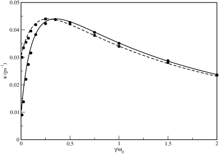
Figure 1: Jump rates in ps^-1 as a function of the coverage (solid line $\theta=0.028$; and dashed line, $\theta=0.18$) for the diffusion of Na atoms on Cu(001) surface at 200 K, along the $[100]$. Kramers results are plotted in lines and mean first passage time calculations are plotted in circles and squares.

In Fig. 2 the tracer diffusion coefficient in a.u. versus the total friction at 200 K is plotted. White circles are issued from the ISA model and black circles from Kramer’s results. The agreement is again quite good and Einstein’s law is clearly fulfilled.

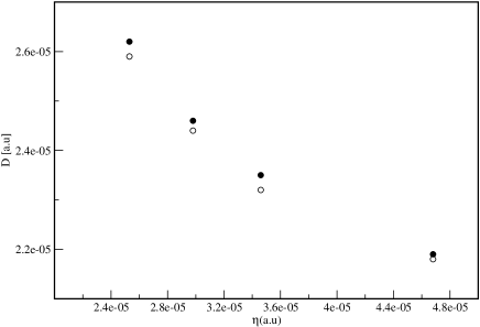
Figure 2: Tracer diffusion coefficient in a. u. as a function of the coverage for the diffusion of Na atoms on Cu(001) surface at 200 K, along the $[100]$. Kramers results are given by black circles and Langevin numerical simulations by white circles.

Finally, in Fig. 3 the FWHM (in $\mu$eV) of the Q-peak is shown for two different coverages (low, 0.028, and moderate, 0.18) at 200 K as a function of the parallel wave vector transfer covering the first Brilloiun zone. Results from the ISA model are plotted in black squares and circles. White squares and circles are experimental results and the solid lines are coming from Kramer’s theory which are also obtained by assuming a Chudley-Elliott model. The agreement among theoretical results is fairly good but with the experimental results are poorer for the high coverage. Values of the coverage around 0.16 mark the upper limit where the ISA model can work.

Figure 3: Full width at half maximum (in $\mu$eV) of the quasielastic peak as a function of the parallel wave vector transfer for the diffusion of Na atoms on Cu(001) surface at 200 K and two coverages: 0.028 (low coverage) and 0.18 (intermediate coverage), along the $[100]$.

III.3.3 Quantum dynamics

Our starting point is again Eq. (27) where now the adiabatic force is derived by any general interaction potential. The same discussion as in the harmonic case can be followed for the $I_{1}$ factor.

For Na atoms, the pairwise interaction potential is repulsive and the mean interparticle distance should be most of the time greater than $\lambda_{B}$. Thus, the $I_{2}$ factor could be replaced, in a first approximation, by the classical counterpart, Eq. (93). The error comes from small times but due to the fact the diffusion process is a long time one, the influence on the quasielastic peak (wave-vector dependence) and quantum diffusion constant (Einstein’s law) will be really small for massive particles ruth5 . In Fig. 4, we show the effects of the quantum correction in the diffusion process studied here at two different surface temperatures for a coverage of 0.028. For comparison, in this plot, the classical intermediate scattering function and the real part of its quantum analog are displayed. As seen, although the Na atom is a relatively massive particle, at low temperatures the plateau is lower for the quantum case. This implies an initially faster decay arising from the strong influence of the quantum behavior at short time scales. It is therefore the real part of the intermediate scattering function what one should compare to the experiment rather than $I_{2}$, as is usually done. Obviously, this effect will be less pronounced at high coverages.

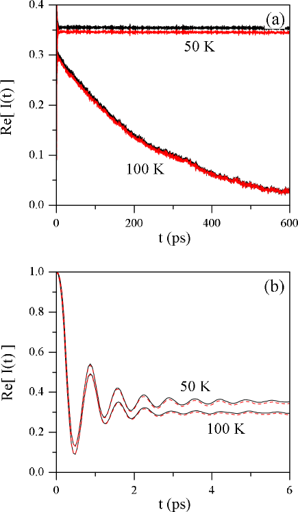
Figure 4: (Color online.) Classical intermediate scattering function (45) for Na diffusion on a Cu(001) surface at 50 K and 100 K (black solid lines) and the real part of its quantum-mechanical analog (51) (red/dark grey dashed lines). The surface coverage considered here is 0.028 and the diffusion along the azimut $[100]$.

At very low temperatures, the Matsubara series should play a similar role like the extra term observed in the $f$ and $g$ functions like in the harmonic case. Thus, a new quantum correction should be added for very low temperatures.

IV Conclusions

It is remarkable that, within the Markovian formalism presented here, the quantum intermediate scattering function, $I_{1}$, is independent of the relative corrugation of the surface and, at short times, also independent of the friction. At low surface temperatures, the $I_{1}$ factor will be responsible for a higher contribution of the imaginary part of $I$, given by Eq. (51), modifying substantially the response in the diffusion process. For relatively heavy particles and at very long times (diffusion time scales), operators in the $I_{2}$ factor can be replaced by variables, since $\lambda_{B}$ is very small. As far as we know, an exact quantum calculation for a corrugated surface is not possible and some approximations have to be invoked, e.g., the damped harmonic oscillator has been applied here in order to obtain close formulas. Of course, other different, alternative theoretical approaches can also be found in literature (see, for example, Refs. peter, ; others, ) but within the single adsorbate approximation. The theoretical formalism that we propose here should also be very useful to avoid extrapolations at zero surface temperature when trying to extract information about the frustrated translational mode. Diffusion experiments at low temperatures are very difficult to perform (or even unaffordable); for example, for the HeSE technique surface temperatures around 100 K can be attainable. However, the type of theoretical calculations needed in this formalism is easy to carry out and they would provide a simple manner to go to lower temperatures with quite reliable results, thus allowing to extract confident values of magnitudes such as friction coefficients and oscillation frequencies. By decreasing the surface temperature, quantum effects are extended at higher values of time. Going from 100 K to 50 K, the time where the quantum dynamics is important increases from 0.07 ps to 0.15 ps. The standard propagation time for diffusion is greater than 400 ps. In our opinion, the limits of applicability of this quantum theory should be at coverages up to 12-16 $\%$ and around 50 K where the Matsubara series is still playing no role on the diffusion. Obviously, at lower surface temperatures, the quantum character of the noise becomes more and more important. This type of conditions as well as the diffusion mediated by tunneling needs to be more investigated since new experimental results are being analyzed.

References

- eprint
- (1) R. G. Gordon, Adv. Mag. Resonance 3 (1968) 1.
- (2) D. A. McQuarrie, Statistical Mechanics, Harper and Row, New York, 1976.
- (3) R. Kubo, Rep. Prog. Phys. 29 (1966) 255.
- (4) L. Van Hove, Phys. Rev. 95 (1954) 249.
- (5) G. H. Vineyard, Phys. Rev. 110 (1958) 999.
- (6) S. W. Lovesey, Theory of Neutron Scattering from Condensed Matter, Clarendon, Oxford, 1984.
- (7) J. P. Hansen, I. R. McDonald, Theory of Simple Liquids, Academic Press, London, 1986.
- (8) M. Bée, Quasielastic Neutron Scattering, Adam Hilger, Bristol, 1988.
- (9) A. M. Lahee, J. R. Manson, J. P. Toennies, Ch. Wöll, Phys. Rev. Lett. 57 (1986) 471; ibid J. Chem. Phys. 86 (1987) 7194.
- (10) J. R. Manson, V. Celli, Phys. Rev. B 39 (1989) 3605.
- (11) F. Hofmann, J. P. Toennies, Chem. Rev. 78 (1996) 3900.
- (12) S. Miret-Artés, E. Pollak, J. Phys.: Condens. Matter 17 (2005) S4133.
- (13) A. P. Graham, F. Hofmann, J. P. Toennies, L. Y. Chen, S. C. Ying, Phys. Rev. B 56 (1997) 10567.
- (14) J. Ellis, A. P. Graham, F. Hofmann, J. P. Toennies, Phys. Rev. B 63 (2001) 195408.
- (15) J. L. Vega, R. Guantes, S. Miret-Artés, J. Phys.: Condens. Matter 14 (2002) 6193.
- (16) J. L. Vega, R. Guantes, S. Miret-Artés, J. Phys.: Condens. Matter 16 (2004) S2879.
- (17) J. L. Vega, R. Guantes, S. Miret-Artés, Phys. Chem. Chem. Phys. 4 (2002) 4985.
- (18) R. Guantes, J. L. Vega, S. Miret-Artés, E. Pollak, J. Chem. Phys. 119 (2003) 2780.
- (19) R. Guantes, J. L. Vega, S. Miret-Artés, E. Pollak, J. Chem. Phys. 120 (2004) 10768.
- (20) R. Martínez-Casado, J. L. Vega, A. S. Sanz, S. Miret-Artés, Phys. Rev. Lett. 98 (2007) 216102.
- (21) R. Martínez-Casado, J. L. Vega, A. S. Sanz, S. Miret-Artés, Phys. Rev. E 75 (2007) 051128.
- (22) R. Martínez-Casado, J. L. Vega, A. S. Sanz, S. Miret-Artés, J. Phys.: Condens. Matter 19 (2007) 305002.
- (23) R. Martínez-Casado, J. L. Vega, A. S. Sanz, S. Miret-Artés, Phys. Rev. B 77 (2008) 115414.
- (24) J. H. van Vleck, V. F. Weisskopf, Rev. Mod. Phys. 17 (1945) 227.
- (25) C. W. Gardiner, Handbook of Stochastic Methods, Springer-Verlag, Berlin, 1983.
- (26) J. Ellis and J. P. Toennies, Phys. Rev. B 56 (1997) 15378.
- (27) H. Hedgeland, P. Fouquet, A. P. Jardine, G. Alexandrowicz, W. Allison, J. Ellis, Nature Phys. 5 (2009) 561.
- (28) R. Martínez-Casado, A. S. Sanz, G. Rojas-Lorenzo, S. Miret-Artés, J. Chem. Phys. 132 (2010) 054704.
- (29) G. Alexandrowicz, A. P. Jardine, H. Hedgeland, W. Allison, J. Ellis, Phys. Rev. Lett. 97 (2006) 156103.
- (30) A. P. Jardine, G. Alexandrowicz, H. Hedgeland, R.D. Diehl, W. Allison, J. Ellis, J. Phys.: Condens. Matter 19 (2007) 305010.
- (31) A. P. Jardine, H. Hedgeland, G. Alexandrowicz, W. Allison, J. Ellis, Prog. Surf. Sci. 84 (2009) 323.
- (32) B. Farago, Physica B 267-268 (1999) 270.
- (33) P. Fouquet, H. Hedgeland, A. Jardine, G. Alexandrowicz, W. Allison, J. Ellis, Physica B 385-386 (2006) 269.
- (34) R. Martínez-Casado, A. S. Sanz, S. Miret-Artés, J. Chem. Phys. 129 (2008) 184704.
- (35) J. P. Boon, S. Yip, Molecular Hydrodynamics, Dover Publications, New York, 1991.
- (36) P. Schofield, Phys. Rev. Lett. 4 (1960) 239.
- (37) V. B. Magalinskii, Sov. Phys. JETP 9 (1959) 1381.
- (38) A. O. Caldeira, A. J. Leggett, Ann. Phys. (N. Y.) 149 (1983) 374; ibid. 153 (1984) 445.
- (39) U. Weiss, Quantum Dissipative Systems, World Scientific, Singapore, 1993.
- (40) G. Ingold, Lec. Notes Phys. 611 (2002) 1.
- (41) R. Guantes, J. L. Vega, S. Miret-Artés, D. A. Micha, J. Chem. Phys. 120 (2004) 10768.
- (42) R. Martínez-Casado, J. L. Vega, A. S. Sanz, S. Miret-Artés, J. Chem. Phys. 126 (2007) 194711.
- (43) J. Ellis, A. P. Graham, J. P. Toennies, Phys. Rev. Lett. 82 (1999) 5072.
- (44) R. Martínez-Casado, J. L. Vega, A. S. Sanz, S. Miret-Artés, J. Phys.: Condens. Matter 19 (2007) 176006.
- (45) H. Risken, The Fokker-Planck Equation, Springer-Verlag, Berlin, 1984.
- (46) C. T. Chudley, R. J. Elliott, Proc. Phys. Soc. 57 (1961) 353.
- (47) V. I. Mel’nikov, S. V. Meshkov, J. Chem. Phys. 85 (1986) 1018; V. I. Mel’nikov, Phys. Rep. 209 (1991) 1.
- (48) E. Pollak, J. Chem. Phys. 85 (1986) 865. Y. Georgievskii, E. Pollak, Phys. Rev. E 49 (1994) 5098: Y. Georgievskii, M. A. Kozhushner, E. Pollak, J. Chem. Phys. 102 (1995) 6908.
- (49) H. A. Kramers, Physica (Utrecht) 7 (1940) 284.
- (50) E. Pollak, H. Grabert, P. Hänggi, J. Chem. Phys. 91 (1989) 4037; P. Hänggi, P. Talkner, M. Borkovec, Rev. Mod. Phys. 62 (1990) 251.
- (51) R. F. Grote, J. T. Hynes, J. Chem. Phys. 73 (1980) 2715.
- (52) M.P. Allen, D.J. Tildesley, Computer Simulation of Liquids, Clarendon, Oxford, 1990.
- (53) L.Y. Chen, S.C. Ying, Phys. Rev. Lett. 73 (1994) 700; Y. Georgievskii, E. Pollak, Phys. Rev. E 49 (1994) 5098.