grmonty: a Monte Carlo Code for Relativistic Radiative Transport

Abstract

We describe a Monte Carlo radiative transport code intended for calculating spectra of hot, optically thin plasmas in full general relativity. The version we describe here is designed to model hot accretion flows in the Kerr metric and therefore incorporates synchrotron emission and absorption, and Compton scattering. The code can be readily generalized, however, to account for other radiative processes and an arbitrary spacetime. We describe a suite of test problems, and demonstrate the expected $N^{-1/2}$ convergence rate, where $N$ is the number of Monte Carlo samples. Finally we illustrate the capabilities of the code with a model calculation, a spectrum of the slowly accreting black hole Sgr A* based on data provided by a numerical general relativistic MHD model of the accreting plasma.

1 Introduction

There is wide interest in calculating the emergent radiation from relativistic astrophysical sources, including accreting black holes, accreting neutron stars, and relativistic blast waves. A variety of methods for solving the radiative transfer problem in these sources have been developed over the last few decades (e.g. Pozdynakov et al., 1983; Górecki & Wilczewski, 1984; Hauschildt & Wehrse, 1991; Carrigan & Katz, 1992; Coppi et al., 1993; Stern et al., 1995; Poutanen & Svensson, 1996; Zane et al., 1996; Dove et al., 1997; Böttcher & Liang, 2001; Schnittman et al., 2006; Noble et al., 2007; Wu et al., 2008), some based on Monte Carlo schemes. Few of these schemes take full account of relativistic effects in the source, however, and this is crucial in estimating the spectra of hot plasma deep in a gravitational potential well, or highly relativistic blast waves. Monte Carlo transport of radiation in accretion flows around compact objects has been considered by (e.g. Schnittman & Krolik, 2009; Schnittman, 2006; Yao et al., 2005; Böttcher et al., 2003; Böttcher & Liang, 2001; Laurent & Titarchuk, 1999; Agol & Blaes, 1996; Stern et al., 1995). Among others, Cullen (2001); Molnar & Birkinshaw (1999); Hua (1997); Górecki & Wilczewski (1984); Pozdynakov et al. (1983) give more general discussions of Monte Carlo radiative transfer techniques.

We were motivated by efforts to model the radio source and black hole candidate Sgr A*. Our interest in this source drove us to develop a numerical scheme that could accurately calculate spectra of a relativistic source in which the plasma properties (velocity, density, magnetic field strength, and temperature) were specified by a separate model—that is, sources in which radiation plays a negligible role in the dynamics and energetics. The result, a Monte Carlo scheme called grmonty, is described in this paper. The spirit of our calculation is to obtain an accurate spectrum with as few approximations as possible. To this end we treat Compton scattering with no expansions in $v/c$, and allow for general angle-dependent emission and absorption (we specialize to thermal synchrotron in this work).

In designing grmonty our philosophy has been to maximize the physical transparency and minimize the length of the code, occasionally at the cost of reduced performance. Sometimes simplicity and efficiency are in harmony. We chose to directly integrate the geodesic equation rather than using a scheme that relies on integrability of geodesics in the Kerr metric. We will show that for radiative transfer problems where many points are required along each geodesic, direct integration is not only simpler and easier to modify, but also faster.

Our paper is organized as follows. In §2 we describe how we sample emission, and in §3 we describe how we track photons along geodesics. Evolution of superphoton weights under absorption is described in §4, and sampling of scattered photons is discussed in §5. Photons at large distance from the source must be sampled and assembled into spectra; this is described in §6. The code has been extensively verified; we describe tests in §7. §8 describes a sample calculation, and §9 summarizes our results.

Throughout this paper we assume that there is an underlying model that can be queried to supply the rest-mass density $\rho_{0}$, the internal energy $u$, the four-velocity $u^{\mu}$, and magnetic field four-vector $b^{\mu}$ for the radiating plasma. Usually we expect the model to be supplied by a numerical simulation in a coordinate basis $x^{\mu}$.

2 Manufacturing Superphotons

Emission in grmonty is treated by sampling the emitted photon field. The samples, here called “superphotons” (also “photon packets”), have weight $w$, coordinates $x^{\mu}$, and wave vector $k^{\mu}$. The weight $w\gg 1$ is a pure number that represents the ratio of photons to superphotons: $dN=wdN_{s}$ ($N_{s}\equiv$ number of superphotons, $N\equiv$ number of photons). In our models the weight is a function of the emitting plasma frame frequency $\nu$ and nothing else. The coordinates are typically in model units (e.g. for a black hole accretion flow calculation, length unit $L=GM/c^{2}$), and the components of $k^{\mu}$ are given in units of $m_{e}c^{2}$.

How should superphotons be distributed over $x^{\mu}$ and $k^{\mu}$? The initial superphoton momentum can be described in an orthonormal tetrad basis $e^{\mu}_{(a)}$ that is attached to the plasma, so that $e^{\mu}_{(t)}=u^{\mu}$ ($\mu$ is the coordinate index, and $(a)$ is the index associated with the tetrad basis, raised and lowered using the Minkowski metric). In the tetrad basis $k^{(a)}$ is specified by frequency $\nu$ and spatial direction unit vector $\hat{\bf n}$ that is contained within the solid angle $d\Omega$. The probability distribution for superphotons is then

$$\frac{1}{{\sqrt{-g}}}\,\frac{dN_{s}}{d^{3}xdt\,d\nu d\Omega}=\frac{1}{w{\sqrt{-g}}}\,\frac{dN}{d^{3}xdt\,d\nu d\Omega}=\frac{1}{w}\frac{j_{\nu}}{h\nu}$$ (1)

where $j_{\nu}$ is the emissivity (always defined in the plasma frame), since ${\sqrt{-g}}\,d^{3}xdt$ is invariant (meaning coordinate invariant). In a time interval $\Delta t$ we expect to create

$$N_{s,tot}=\Delta t\int\;{\sqrt{-g}}\;d^{3}x\;d\nu\;d\Omega\frac{1}{w}\frac{j_{\nu}}{h\nu}$$ (2)

superphotons over the entire model volume. The total computational effort is proportional to $N_{s,tot}$, so we control the computational effort by scaling the weights.

How should we distribute superphotons over the volume? grmonty subdivides the model volume into volume elements (“zones”) of size $\Delta^{3}x$ (e.g. in Boyer-Lindquist $t,r,\theta,\phi$ coordinates for the Kerr metric, $\Delta r\Delta\theta\Delta\phi$). For zone $i$ we expect

$$N_{s,i}=\Delta t\Delta^{3}x{\sqrt{-g}}\int\;d\nu\;d\Omega\;\frac{1}{w}\,\frac{j_{\nu}}{h\nu}$$ (3)

to be created in time $\Delta t$. We create $N_{s,i}$ superphotons at the center of zone $i$. Fractional $N_{s,i}$ are dealt with by rejection sampling.

The momentum-space (wave vector) piece of the probability distribution (1) can be sampled by techniques outlined below to give $\nu$ and $\hat{\bf n}$. With $x^{\mu}$, $\nu$ and $\hat{\bf n}$ in hand, we can construct $k^{(a)}$ and, finally, transform to the coordinate basis $e^{\mu}_{(a)}k^{(a)}=k^{\mu}$.

The remaining ingredients in the sampling procedure are the emissivity, the orthonormal tetrads, and the sampling procedures for $\nu$ and $\hat{\bf n}$.

2.1 Emissivity

grmonty depends on the emissivity only through functions that specify $j_{\nu}$ and $\int d\nu d\Omega j_{\nu}/\nu$, so it is straightforward to include any emission/absorption process.

In our target problem the only source of superphotons is thermal synchrotron emission at dimensionless temperature $\Theta_{e}\equiv kT_{e}/(m_{e}c^{2})$. Leung et al. (2009) show that, for $\Theta_{e}\gtrsim 0.5$,

$$j_{\nu}(\nu,\theta) \simeq\frac{\sqrt{2}\pi e^{2}n_{e}\nu_{s}}{3cK_{2}(\Theta_{e}^{-1})}\left(X^{1/2}+2^{11/12}X^{1/6}\right)^{2}\exp\left(-X^{1/3}\right)$$ (4a)

$$X \equiv\frac{\nu}{\nu_{s}}$$ (4b)

$$\nu_{s} \equiv\frac{2}{9}\left(\frac{eB}{2\pi m_{e}c}\right)\Theta_{e}^{2}\sin\theta$$ (4c)

where $K_{2}$ is the modified Bessel function of the second kind, $n_{e}$ is the number density of electrons, $B$ is the magnetic field strength, and $\theta$ is the angle between the wave vector and magnetic field. For large $\Theta_{e}$, $K_{2}(\Theta_{e}^{-1})\simeq 2\Theta_{e}^{2}$, but for $\Theta_{e}\lesssim 1$ better agreement with the emissivities of Leung et al. (2009) is obtained if $K_{2}$ is evaluated directly. Since the emissivity must be evaluated many times, it is most efficient to precompute $K_{2}(\Theta_{e}^{-1})$ at the beginning of the calculation and store the results in a table.

2.2 Orthonormal tetrads

The wave vector sampling is done in an orthonormal tetrad attached to the fluid. We construct the orthonormal tetrad $e^{\mu}_{(a)}$ using numerical Gram-Schmidt orthogonalization. Here $\mu$ is the coordinate index, and $(a)$ is the index associated with the tetrad basis, which is raised and lowered using the Minkowski metric.

We set $e^{\mu}_{(0)}=u^{\mu}$ ($u^{\mu}\equiv$ plasma four-velocity), and then use $b^{\mu}$, the magnetic field four-vector, as the first trial vector (this is numerically convenient since we will want to orient wave vectors with respect to the magnetic field; if $b^{\mu}=0$ then we use a default, radius-aligned, trial vector). Thus $e^{\mu}_{(1)}={\rm NORM}\left(b^{\mu}-e^{\mu}_{(0)}(e^{\nu}_{(0)}b_{\nu})\right)$ (${\rm NORM}$: normalize). The process is repeated with additional trial vectors to create a full tetrad basis.

The tetrad-to-coordinate basis transformation is

$$k^{\mu}=e^{\mu}_{(a)}k^{(a)}$$ (5)

and the coordinate to tetrad transformation is

$$k^{(a)}=e^{(a)}_{\mu}k^{\mu}.$$ (6)

With these transformations in hand, we can construct the superphoton wave vector in the orthonormal frame and then transform it to the coordinate basis.

2.3 Wave vector sampling procedure

2.3.1 Photon energy

Within zone $i$ superphotons are distributed over frequency according to the distribution

$$\frac{dN_{s,i}}{d\ln\nu}=\Delta t\Delta^{3}x{\sqrt{-g}}\;\frac{1}{h\,w}\;\int d\Omega\;j_{\nu}.$$ (7)

We sample the distribution only between a minimum and maximum frequency $\nu_{min}$ and $\nu_{max}$. These must be chosen so that no significant emission is omitted from the final spectrum.

We distribute superphotons over frequency by rejection sampling. For simplicity, we use a constant envelope function equal to the maximum of Equation (7) (for zone $i$). Thus we draw tentative values uniformly in $\ln\nu$ from $\nu_{min}$ to $\nu_{max}$. The efficiency of the sampling procedure is the ratio of the areas under the distribution and envelope, so if the distribution given in Equation (7) is sharply peaked this technique can be inefficient.

In practice, we choose a tentative frequency $\nu_{0}=\exp(r_{1}\ln{\nu_{max}/\nu_{min}}+\ln{\nu_{min}})$, where $r_{1}$ is drawn from a uniform distribution on [0,1) (we use the Mersenne twister random number generator from the GNU Scientific Library, hereafter GSL). A second number $r_{2}$ is drawn from [0,1) and the process is repeated until

$$r_{2}<\left.{\left.\frac{dN_{s,i}}{d\ln\nu}\right|}_{\nu_{0}}\right/\mathrm{MAX}\left(\frac{dN_{s,i}}{d\ln\nu}\right).$$ (8)

The efficiency of this process is $\sim 15\%$, but the cost is small compared to the total cost of grmonty.

2.3.2 Photon direction

The superphoton direction $\hat{\bf n}$ is described by polar coordinates $\theta$ and $\phi$ in the tetrad frame, where $\theta$ is the angle between the spatial part of the wave vector and the magnetic field. The colatitude $\theta$ is obtained by rejection sampling: a tentative value for $\theta$ is obtained by drawing $\mu=\cos\theta$ from a uniform distribution on [-1,1), a second number $r$ is drawn from a uniform distribution on [0,1), and $\theta$ is accepted if

$$r<\frac{j_{\nu}(\theta)}{j_{\nu}(\pi/2)}$$ (9)

(this procedure is specific to the synchrotron emissivity). The efficiency of this scheme is problem dependent; for our target application the efficiency is $\sim 65\%$. Finally, $\phi$ is drawn from a uniform distribution on [0,2$\pi$).

2.3.3 Transformation to coordinate frame

Once $\theta$, $\phi$, and ${\epsilon}=h\nu/m_{e}c^{2}$ are selected, the wave vector is completely specified in the orthonormal tetrad frame:

$$k^{(0)} ={\epsilon}$$ (10a)

$$k^{(1)} ={\epsilon}\cos\theta$$ (10b)

$$k^{(2)} ={\epsilon}\sin\theta\cos\phi$$ (10c)

$$k^{(3)} ={\epsilon}\sin\theta\sin\phi,$$ (10d)

and the wave vector in the coordinate frame is $k^{\mu}=e^{\mu}_{(a)}k^{(a)}$.

3 Geodesic Integration

General relativistic radiative transfer differs from conventional radiative transfer in Minkowski space in that photon trajectories are no longer trivial; photons move along geodesics. Tracking geodesics is a significant computational expense in grmonty.

The governing equations for a photon trajectory are

$$\frac{dx^{\alpha}}{d\lambda}=k^{\alpha}$$ (11)

which defines $\lambda$, the affine parameter, the geodesic equation

$$\frac{dk^{\alpha}}{d\lambda}=-\Gamma^{\alpha}_{\mu\nu}k^{\mu}k^{\nu}$$ (12)

and the definition of the connection coefficients

$$\Gamma^{\alpha}_{\mu\nu}=\frac{1}{2}g^{\alpha\gamma}\left(g_{\gamma\mu,\nu}+g_{\gamma\nu,\mu}-g_{\mu\nu,\gamma}\right)$$ (13)

in a coordinate basis.

We assume nothing about the metric, so it is easy to change coordinate systems and even to extend the code to dynamical spacetimes. Nevertheless, our main application—to black hole accretion flows—is in the Kerr metric, where geodesics are integrable. The four constants of the motion are the energy-at-infinity $E$ (in Boyer-Lindquist coordinates $t,r,\theta,\phi$, $E=-k_{t}$), the angular momentum $l=k_{\phi}$, Carter’s constant $Q=k_{\theta}^{2}+k_{\phi}^{2}\cot^{2}\theta-a^{2}k_{t}^{2}\cos^{2}\theta$ (see Carter, 1968), and the condition that $k^{\alpha}$ be null: $k^{\mu}k_{\mu}=0$, equivalent to the dispersion relation for photons in vacuo: $\omega^{2}=c^{2}k^{2}$. These four constants of the motion can be used to quasi-analytically obtain $x^{\mu}$ and $k^{\mu}$ in terms of an initial (or final) position and wave vector (see, e.g., Rauch & Blandford, 1994; Beckwith & Done, 2005; Dexter & Agol, 2009).

The integrability of geodesics in the Kerr metric would appear to provide an opportunity for significant computational economies. We show below, however, that direct integration of equations (11) and (12) is not only simpler and more flexible but also faster than at least one implementation of an integral-based technique.

Which ODE integration algorithm is best for the geodesic equation? If only a few coordinate evaluations are required over the entire geodesic then a high order scheme is optimal. For example, we have found that the embedded Runge-Kutta Prince-Dorman method available in GSL is fast and accurate; it can easily be made to conserve the integrals of motion to machine precision. Many coordinate evaluations are required, however, when integrating the equation of radiative transfer, as grmonty does, along superphoton trajectories. A second order scheme can then provide the required accuracy at minimal cost.

Evaluating the connection coefficients is expensive, so we want to choose a scheme that minimizes the number of evaluations. The velocity Verlet algorithm, which for the geodesic equation is

$$x^{\alpha}_{n+1} =x^{\alpha}_{n}+k^{\alpha}_{n}\Delta\lambda+{{1}\over{2}}\left({{dk^{\alpha}}\over{d\lambda}}\right)_{n}(\Delta\lambda)^{2}$$ (14a)

$$k^{\alpha}_{n+1,p} =k^{\alpha}_{n}+\left({{dk^{\alpha}}\over{d\lambda}}\right)_{n}\Delta\lambda$$ (14b)

$$\left({{dk^{\alpha}}\over{d\lambda}}\right)_{n+1} =-\Gamma^{\alpha}_{\mu\nu}(\mathbf{x}_{n+1})k^{\mu}_{n+1,p}k^{\nu}_{n+1,p}$$ (14c)

$$k^{\alpha}_{n+1} =k^{\alpha}_{n}+{{1}\over{2}}\left(\left({{dk^{\alpha}}\over{d\lambda}}\right)_{n}+\left({{dk^{\alpha}}\over{d\lambda}}\right)_{n+1}\right)(\Delta\lambda),$$ (14d)

requires only one evaluation of the connection coefficients per step. Accuracy can be improved by using the result of equation (14d) to recompute the derivative equation (14c) with $k^{\mu}_{n+1,p}=k^{\mu}_{n+1}$ and then reevaluating equation (14d). This process is repeated until the change in the wave vector between estimates is below some tolerance. In grmonty  we continue this iteration until the fractional change is less than $10^{-3}$ (typically only once or twice). This does not require any additional evaluations of $\Gamma^{\alpha}_{\mu\nu}$. Very rarely we find that this iteration fails to converge, and then grmonty defaults to taking the step with a classical $4^{\rm th}$-order Runge-Kutta technique.

How fast and accurate is our geodesic integration scheme? We propose the following benchmark. Consider a point on a direct, circular, marginally stable orbit in the equatorial plane of a black hole with spin $a/M=1-2^{-4}=0.9375$ that emits radiation isotropically in its rest frame. Sample the emitted photons (in a Monte Carlo sense; the analytic circular orbit orthonormal tetrads available in Bardeen et al. (1972) are useful for constructing the initial wave vectors) and track them until they cross the horizon or reach $rc^{2}/(GM)=100$ ($r$ is the Boyer-Lindquist or Kerr-Schild radial coordinate). Figure 1 shows as dots a representative sample of photon geodesics from grmonty in the coordinate frame, illustrating the effects of relativistic beaming, lensing, and frame dragging.

Second order convergence of the velocity Verlet integration scheme is demonstrated in Figure 2, which plots the average fractional error in $E$, $l$, and $Q$ as a function of a step-size parameter $\varepsilon$. We typically set $\varepsilon=0.04$ as a compromise between performance and accuracy; the average fractional errors at the end of the integrations are $\sim 2\times 10^{-3}$, $\sim 4\times 10^{-2}$, and $\sim 8\times 10^{-2}$ for $E$, $l$, and $Q$, respectively. We have verified that this choice makes geodesic tracking errors subdominant in the error budget for the overall spectrum.

With $\varepsilon=0.04$, grmonty integrates $\sim 16,700\textrm{ geodesics sec}^{-1}$ on a single core of an Intel Xeon model E5430. If we use $4^{\rm th}$-order Runge-Kutta exclusively so that the error in $E$, $l$, and $Q$ is $\sim$1000 times smaller, then the speed is $\sim 6,200\textrm{ geodesics sec}^{-1}$. If we use the Runge-Kutta Prince-Dorman method in GSL with $\varepsilon=0.04$ the fraction error is $\sim 10^{-10}$ and the speed is $\sim 1,700\textrm{ geodesics sec}^{-1}$. These results can be compared to the publicly available integral-based geokerr code of Dexter & Agol (2009), whose geodesics are shown as the (more accurate) solid lines in Figure 1. If we use geokerr to sample each geodesic the same number of times as grmonty ($\sim 180$), then on the same machine geokerr runs at $\sim 1,000\textrm{ geodesics sec}^{-1}$. It is possible that other implementations of an integral-of-motion based geodesic tracker could be faster.

If only the initial and final states of the photon are required, we find that geokerr computes $\sim 77,000\textrm{ geodesics sec}^{-1}$. The adaptive Runge-Kutta Cash-Karp integrator in GSL computes $\sim 34,500\textrm{ geodesics sec}^{-1}$ with fractional error $\sim 10^{-3}$.

4 Absorption

grmonty treats absorption deterministically. We begin with the radiative transfer equation written in the covariant form

$$\frac{1}{{\mathcal{C}}}\frac{d}{d\lambda}\left(\frac{I_{\nu}}{\nu^{3}}\right)=\left(\frac{j_{\nu}}{\nu^{2}}\right)-(\nu\alpha_{\nu,a})\left(\frac{I_{\nu}}{\nu^{3}}\right).$$ (15)

(see Mihalas & Mihalas, 1984). Here $I_{\nu}$ is specific intensity and $\alpha_{\nu,a}$ is the absorption coefficient (which is always evaluated in the fluid frame). The absorption coefficient must be computed by a separate subroutine; for thermal synchrotron emission we set $\alpha_{\nu,a}=j_{\nu}/B_{\nu}$. ${\mathcal{C}}$ is a constant that depends on the units of $k^{\mu}$ (in grmonty, electron rest mass), $\nu$ (Hertz), and the length unit $L$ for the simulation in cgs units. For grmonty

$${\mathcal{C}}=\frac{Lh}{m_{e}c^{2}}.$$ (16)

Each quantity in parentheses in equation (15) is invariant; $I_{\nu}/\nu^{3}$, for example, is proportional to the photon phase space density.

Since $I_{\nu}/\nu^{3}$ is proportional to the number of photons moving along each ray, $I_{\nu}/\nu^{3}\propto w$, and equation (15) implies (ignoring emission)

$$\frac{dw}{d\tau_{a}}=-w$$ (17)

where

$$d\tau_{a}=(\nu\alpha_{\nu,a})\;{\mathcal{C}}d\lambda$$ (18)

is the differential optical depth to absorption and the quantity in parentheses is the “invariant opacity.” This equation we integrate with second order accuracy

$$\tau_{a}=\frac{1}{2}\left((\nu\alpha_{\nu,a})_{n}+(\nu\alpha_{\nu,a})_{n+1}\right)\;{\mathcal{C}}\Delta\lambda,$$ (19)

and then set

$$w_{n+1}=w_{n}e^{-\tau_{a}}.$$ (20)

Since the components of $k^{\mu}$ are expressed in units of the electron rest-mass energy, $\nu=-k^{\mu}u_{\mu}m_{e}c^{2}/h$. Storing the invariant opacity at the end of each step saves computations since it can be reused as the beginning of the following step.

5 Scattering

Our treatment of scattering consists of two parts: the first determines where a superphoton should scatter and the second determines the energy and direction of the scattered superphoton.

5.1 Selection of scattering optical depth

When a superphoton is created or scattered grmonty selects the scattering optical depth $\tau_{s}$ at which the next scattering event will take place. Scattering follows the cumulative probability distribution

$$p=1-e^{-\tau_{s}}=\tau_{s}+O(\tau_{s}^{2}),$$ (21)

so superphotons will experience on average $\tau_{s}$ scattering events when $\tau_{s}\lesssim 1$. In optically thin sources this would result in poor signal to noise in portions of the spectrum dominated by scattered light. To overcome this, we use the biased probability distribution

$$p=1-e^{-b\tau_{s}}$$ (22)

where $b$ is a bias parameter. This technique was originally proposed by Kahn (1950) in the context of deep penetration of neutrons in radiation shielding and has since been extensively explored in the nuclear engineering literature (often refered to as exponential biasing or exponential transform). Whereas in deep penetration problems $b\leq 1$ in order to allow for sampling of radiation at high optical depths, here we set $b\geq 1$ in order to better sample scattered photons at low optical depths. Superphotons now experience on average $b\tau_{s}$ scattering events. Two superphotons emerge from a scattering event: the incident superphoton of weight $w$ and a new scattered superphoton. For conservative scattering the incident superphoton has its weight reset to $w(1-1/b)$ and the new superphoton has weight $w/b$, so that weight (photon number) is conserved.

What should we choose for the bias parameter $b$? The goal is to set $b$ such that scattering is more likely to occur in regions which contribute most to the spectrum. This is an example of the more general technique of importance sampling. Typically we set the bias parameter $b=\mathrm{MAX}(1,\alpha\Theta_{e}^{2}/\tau_{s,max})$ ($\alpha$ is a scaling factor we set to $1/{\langle}\Theta_{e}{\rangle}^{2}$ where ${\langle}\Theta_{e}{\rangle}$ is the volume averaged dimensionless temperature and $\tau_{s,max}$ is an estimated maximum scattering optical depth) to improve sampling on the high energy side of each scattering order, which is populated by photons scattered from high temperature plasma. If the bias factor is too large a “chain reaction” results in an exponentially growing number of superphotons; $1/\tau_{s,max}$ is an estimate of the critical bias factor in a $\Theta_{e}=1$ plasma.

We evaluate the scattering optical depth along geodesics in a manner analogous to the absorption optical depth;

$$\tau_{s}=\frac{1}{2}\left((\nu\alpha_{\nu,s})_{n}+(\nu\alpha_{\nu,s})_{n+1}\right)\;{\mathcal{C}}\Delta\lambda,$$ (23)

is the scattering depth along a step.

5.1.1 Covariant evaluation of extinction coefficient

In our applications electron scattering dominates. The general, invariant expression for the rate of binary interactions $dN_{ab}$ between a population of particles $dN_{a}$ and $dN_{b}$ is

$$\frac{1}{{\sqrt{-g}}}\,\frac{dN_{ab}}{d^{3}xdt}=\frac{1}{1+\delta_{ab}}\;\int\;\frac{d^{3}p_{a}}{{\sqrt{-g}}\,p_{a}^{t}}\;\frac{d^{3}p_{b}}{{\sqrt{-g}}\,p_{b}^{t}}\;\frac{dN_{a}}{d^{3}x\,d^{3}p_{a}}\;\frac{dN_{b}}{d^{3}x\,d^{3}p_{b}}\;(-p_{a\mu}p_{b}^{\mu})\;\sigma v_{ab}$$ (24)

where $\delta_{ab}$ prevents double-counting if $a=b$, $d^{3}p=dp_{1}dp_{2}dp_{3}$, $\sigma$ is the invariant cross section, and $v_{ab}=c(1+m_{a}^{2}m_{b}^{2}/(-p_{a\mu}p_{b}^{\mu})^{2})^{1/2}$. This is the manifestly covariant generalization of equation (12.7) of Landau & Lifshitz (1975).

We want to use this expression to find the cross section for a photon with wavevector $k_{0}^{\mu}$ interacting with a population of particles of mass $m>0$. We therefore set $dN_{\gamma}/d^{3}xd^{3}p=\delta(k^{\mu}-k_{0}^{\mu})$ and, dropping the subscripts on $k$ and $p$, the integral reduces to

$$\frac{1}{{\sqrt{-g}}}\,\frac{dN_{m\gamma}}{d^{3}xdt}=\int\;\frac{d^{3}p}{{\sqrt{-g}}\,p^{t}}\;\frac{dn_{m}}{d^{3}p}\;\frac{(-k_{\mu}p^{\mu})}{k^{t}}\;\sigma c$$ (25)

where $dn_{m}=dN_{m}/d^{3}x$. In Minkowski coordinates (${\sqrt{-g}}=1$), define $\beta_{m}\equiv$ the particle speed in the plasma frame and $\mu_{m}\equiv$ the cosine of the angle between the particle momentum and photon momentum in the plasma frame. Then

$$\frac{dn_{m\gamma}}{dt}=\int\;d^{3}p\;\frac{dn_{m}}{d^{3}p}\;(1-\mu_{m}\beta_{m})\;\sigma c.$$ (26)

It is convenient to rewrite this rate in terms of a “hot cross section”

$$\sigma_{h}\equiv{1\over{n_{m}}}\int\;d^{3}p\;\frac{dn_{m}}{d^{3}p}\;(1-\mu_{m}\beta_{m})\;\sigma$$ (27)

so that the interaction rate for a single photon is $n_{m}\sigma_{h}c$ and the extinction coefficient is

$$\alpha_{\nu}=n_{m}\sigma_{h}.$$ (28)

So far we have assumed nothing about the interaction process.

5.1.2 Electron scattering

For electron scattering the cross section is the Klein-Nishina total cross section expressed in terms of the photon energy in the electron rest frame $\equiv{\epsilon}_{e}={\epsilon}\gamma_{e}(1-\mu_{e}\beta_{e})$, ($\gamma_{e}\equiv(1-\beta_{e}^{2})^{-1/2}$ and we have substituted the subscript $e$ for $m$):

$$\sigma_{KN}=\sigma_{T}\frac{3}{4{\epsilon}_{e}^{2}}\left(2+\frac{{\epsilon}_{e}^{2}(1+{\epsilon}_{e})}{(1+2{\epsilon}_{e})^{2}}+\frac{{\epsilon}_{e}^{2}-2{\epsilon}_{e}-2}{2{\epsilon}_{e}}\log(1+2{\epsilon}_{e})\right).$$ (29)

Here $\sigma_{T}$ is the Thomson cross section. For ${\epsilon}\ll 1$,

$$\sigma_{KN}=\sigma_{T}(1-2{\epsilon}+O({\epsilon}^{2}))$$ (30)

which is numerically stable for small ${\epsilon}$, unlike equation (29).

Typically we assume a thermal electron distribution,

$$\frac{dn_{e}}{d\gamma_{e}}=\frac{n_{e}}{\Theta_{e}}\frac{\gamma_{e}^{2}\beta_{e}}{K_{2}(\Theta_{e}^{-1})}\exp\left(-\frac{\gamma}{\Theta_{e}}\right),$$ (31)

and evaluate (27) by direct integration to obtain $\sigma_{h}(\Theta_{e},{\epsilon})$. It is efficient to store the resulting cross sections in a two-dimensional lookup table at the beginning of the calculation. Our $\sigma_{h}$ agrees with Wienke (1985).

5.2 Scattering kernel

Once it is determined that a superphoton should be scattered at an event $x^{\mu}_{s}$, the superphoton is passed to a scattering kernel which processes the scattering event according to the following procedure. Only unpolarized light is considered.

First, a plasma frame orthonormal tetrad is constructed by the same Gram-Schmidt orthogonalization procedure described in §2, and the old superphoton wave vector is transformed from the coordinate frame to the tetrad frame.

Second, a scattering electron is selected. We use the procedure described by Canfield et al. (1987), which selects the four-momentum $p^{\mu}_{e}$ of the scattering electron with an efficiency of $72\%$ at $\Theta_{e}=1$ and nearly $100\%$ for $\Theta_{e}\ll 1$ or $\Theta_{e}\gg 1$ (Canfield et al., 1987).

Third, we boost from the plasma frame tetrad to an electron frame tetrad $q_{(a)}^{\mu}$ and construct the scattered photon wave vector in this frame. The differential scattering cross section is sampled for the scattered photon energy ${\epsilon}_{e}^{\prime}$ and the scattering angle $\theta$. For low energy photons (${\epsilon}_{e}<{\epsilon}_{l}$; in grmonty  ${\epsilon}_{l}=10^{-4}$) the scattering is approximately elastic, so we set ${\epsilon}_{e}^{\prime}={\epsilon}_{e}$ and sample the Thomson differential cross section

$$\frac{2\pi}{\sigma_{T}}\frac{d\sigma_{T}}{d\cos\theta}=\frac{3}{8}(1+\cos^{2}\theta)$$ (32)

for the scattering angle $\theta$ using a rejection scheme. For ${\epsilon}_{e}>{\epsilon}_{l}$ we sample the Klein-Nishina differential cross section

$$\frac{2\pi}{\sigma_{T}}{{d\sigma_{KN}}\over{d{\epsilon}_{e}^{\prime}}}={1\over{{\epsilon}_{e}^{2}}}({{\epsilon}_{e}\over{{\epsilon}_{e}^{\prime}}}+{{\epsilon}_{e}^{\prime}\over{{\epsilon}_{e}}}-1+\cos^{2}\theta),$$ (33)

for ${\epsilon}_{e}^{\prime}$ using a rejection scheme. Here $\cos\theta=1+1/{\epsilon}_{e}-1/{\epsilon}_{e}^{\prime}$. This procedure is inefficient for ${\epsilon}_{e}\gg 1$, but in our target application such large photon energies are rare. Drawing a final angle $\phi$ from a uniform distribution on $[0,2\pi)$ completes the specification of the photon wave vector

$$k^{(0)} ={\epsilon}_{e}^{\prime}$$ (34a)

$$k^{(1)} ={\epsilon}_{e}^{\prime}\cos\theta$$ (34b)

$$k^{(2)} ={\epsilon}_{e}^{\prime}\sin\theta\cos\phi$$ (34c)

$$k^{(3)} ={\epsilon}_{e}^{\prime}\sin\theta\sin\phi$$ (34d)

in the electron-frame tetrad basis $q_{(a)}^{\mu}$; $q_{(1)}$ is aligned parallel to the spatial part of the incoming photon wave vector.

Finally, we boost back from the electron-frame tetrad to the plasma frame tetrad (some of these steps are combined in our code for computational efficiency), and use the plasma frame basis vectors to obtain the coordinate frame scattered photon wave vector $k^{\prime}_{\mu}$.

6 Spectra

Spectra can be measured using a “detector” with area $\Delta A$ at distance $R$, frequency channels of logarithmic width $\Delta\ln\nu$, and integration times $\Delta T$. The flux density in frequency bin $i$ is then just

$$F_{\nu,i}=\frac{1}{\nu_{i}\Delta\ln\nu\;\Delta T\;\Delta A}\sum_{j}w_{j}(h\nu)_{j}$$ (35)

where the sum is taken over all superphotons $j$ that land in the channel during the integration. In principle a software detector can behave just like a physical detector, producing time-dependent spectra from time-dependent flow models. In practice time-dependent models are not (yet) treated self-consistently.

To see why, consider a time-dependent model based on a general relativistic magnetohydrodynamics (GRMHD) model of a black hole accretion flow. Self-consistent treatment of the radiation field would require generating and tracking superphotons through the simulation data as it evolves, i.e. coupling the grmonty to the GRMHD code (the simulation data could be stored and post-processed, but this would require storing almost every timestep and would be impractical and inefficient). The mean number of superphotons tracked simultaneously would depend on the desired signal-to-noise in the final spectrum, as well as the time and energy resolution. Our experience suggests that for nominal energy resolution, signal-to-noise, and time resolution of order the horizon light crossing time, $\sim 10^{8}$ superphotons would need to be maintained within the simulation for the duration of the evolution. The total number required is then $N_{tot}\gg 10^{8}$ and is currently inaccessible without significant computational resources. We plan to attempt this calculation later.

For now we construct spectra of time-dependent data using a stationary-data (or “fast-light”) approximation: each time-slice of data is treated as if it were stationary (time-independent). The slice emits superphotons for a time $\Delta t$. The photons then propagate through the slice data (as $t$ varies along a geodesic the fluid variables are held fixed) and are detected at large distance. The time-steady flux is obtained by substituting $\Delta t$ for $\Delta T$ in equation (35).

6.1 Measuring $\nu L_{\nu}$

In practice we measured $\nu L_{\nu,i}$ rather than $F_{\nu,i}$. Since $\nu L_{\nu}=4\pi R^{2}\nu F_{\nu}$, and $R^{2}/\Delta A$ is the solid angle $\Delta\Omega$ occupied by the detector,

$$\nu L_{\nu,i}={4\pi\over{\Delta\Omega\Delta t}}{1\over{\Delta\ln\nu}}\;\sum_{j}w_{j}h\nu_{j}.$$ (36)

Typically our “detectors” capture all the superphotons in a large angular bin $\Delta\Omega$ around the source. For example, in studies of axisymmetric black hole accretion flows the angular bins capture all photons with Boyer-Lindquist $r>100GM/c^{2}$, $\theta_{n}<\theta<\theta_{n+1}$, independent of $\phi$, where $\theta_{n}$ are the bin boundaries.

We can also estimate average values for any quantity $Q$ associated with emission from a source (e.g. the absorption optical depth). We define the weight-averaged value of $Q$ via

$${\langle}Q{\rangle}\equiv{{\sum Qw}\over{\sum w}},$$ (37)

where the sum is taken within an energy and angular bin.

6.2 Optimal weights

The fractional variance in the Monte Carlo estimate for $\nu L_{\nu}$ is proportional to $\overline{w^{2}}/(\overline{N_{s}}\overline{w}^{2})$, where overline means expectation value and $N_{s}$ is the number of superphotons in the bin. Evidently the optimal weighting of superphotons is achieved when (1) the weights of superphotons are the same within bins, and (2) the superphotons are evenly distributed across frequency bins.

If, as we created new superphotons, we knew $\nu L_{\nu}$, then we could set

$$w_{\nu}=\frac{1}{\overline{N_{s}}h}\;L_{\nu}\Delta\ln\nu$$ (38)

and set $\overline{N_{s}}=N_{s,tot}/N_{b}$, where $N_{b}$ is the number of frequency bins.

Of course we do not know $L_{\nu}$, but for the special case of an optically thin emitting plasma we can estimate it:

$$L_{\nu}\approx\int d^{3}x\sqrt{-g}\int d\Omega\;j_{\nu}$$ (39)

This estimate assumes that all photons escape to infinity, and it ignores Doppler shift, gravitational redshift, scattering, and angular structure in $\nu L_{\nu}$. Nevertheless it is useful because (1) it can be calculated before the Monte Carlo calculation begins; (2) it is far better to use the information contained in this rough estimate of the spectrum than to proceed using, e.g., uniform weights.

7 Tests

We verify the accuracy of grmonty by comparing spectra produced on idealized problems against a reference spectrum $(\nu L_{\nu})_{ref}$ computed analytically (when possible) or computed by an independent code. For all tests we use the following error norm, which effectively measures the maximum of the fractional error, compared to the reference solution, over frequency:

$${\langle\epsilon\rangle}=\frac{1}{\Delta\ln\nu}\int_{\nu_{min}}^{\nu_{max}}\frac{|(\nu L_{\nu})_{{\tt grmonty}}-(\nu L_{\nu})_{ref}|}{(\nu L_{\nu})_{ref}}d\ln\nu$$ (40)

where $\Delta\ln\nu=\ln(\nu_{max}/\nu_{min})$ is the range of integration. The range of integration is the same as plotted in the spectra for each test.

7.1 Optically thin synchrotron sphere

First we consider emission from a homogeneous, optically thin spherical cloud of unit volume threaded by a vertical magnetic field in flat space. The cloud parameters are $\Theta_{e}=100$, $B=1\textrm{ G}$, and $n_{e}=10^{15}\textrm{ cm}^{-3}$, which gives an optical depth at $\nu=10^{9}\textrm{ Hz}$ of $\sim 10^{-2}$ perpendicular to the magnetic field. The emissivity and absorptivity are constant along any line of sight, so

$$I_{\nu}=\frac{j_{\nu}}{\alpha_{\nu}}(1-e^{-\alpha_{\nu}L})\approx j_{\nu}L+O(\tau_{a}^{2})$$ (41)

where $L$ is the path length through the sphere. We numerically integrate this expression over detector solid angle to compute the spectral energy distribution, and compare with the spectrum grmonty produces in Figure 3. Evidently the result is unbiased. Figure 4 demonstrates that grmonty converges on the correct solution as $\propto N^{-1/2}$.

7.2 Optically thick synchrotron sphere

The second test is identical except that the electron number density and therefore the optical depth are increased by a factor of $10^{5}$. The intensity along any line of sight is again

$$I_{\nu}=\frac{j_{\nu}}{\alpha_{\nu}}(1-e^{-\alpha_{\nu}L})$$ (42)

The emitting region becomes optically thick when $(j_{\nu}/B_{\nu})L\gtrsim 1$. For the thermal synchrotron emissivity we use, this occurs below a critical frequency.

The spectrum is shown in Figure 5 and the convergence is shown in Figure 6. The figures make two key points: convergence is slow for small numbers of superphotons; and the overall magnitude of the error is larger than in the optically thin case shown in Figure 4.

The slow initial convergence is due to the large optical depth at some frequencies. When the optical depth is large no superphotons of appreciable weight are recorded until some superphotons have been created in the fraction $\sim 1/\tau$ of the volume that lies within the photosphere. Our problem has $\tau\sim 10^{5}$ at $\nu\sim 10^{8}\textrm{ Hz}$. Since ${\langle\epsilon\rangle}$ effectively measures the maximum of the error over frequency, it is not surprising that grmonty requires $\sim 10^{6}$ superphotons before it begins to converge as $N^{-1/2}$.

7.3 Comptonization of soft photons in a spherical cloud of plasma

This test is based on a problem posed in §6 of Pozdynakov et al. (1983): the spectrum of a spherical, homogeneous, unmagnetized cloud of radius $R$ that contains thermal electrons at density $n_{e}$ and temperature $T_{e}$ that scatter light from a central, thermal source of temperature $T_{s}$. Absorption and emission in the cloud are neglected. The dimensionless parameters of the problem are $\Theta_{e}=kT_{e}/(m_{e}c^{2})$, $\tau=R\sigma_{T}n_{e}$, and $\Theta_{s}=kT_{s}/(m_{e}c^{2})$.

For this test our reference spectrum is computed with an implementation of Pozdnyakov et al.’s Monte Carlo scheme kindly provided by S. Davis. This code, sphere, has been modified in two ways: we have replaced the approximate hot cross sections defined in Pozdynakov et al. (1983) with our more exact, numerically integrated values, and we use the exact Klein-Nishina cross section equation (29) when choosing the electron with which a photon should scatter. Without these changes to sphere differences between the spectra are $\lesssim 1\%$, consistent with the error Pozdynakov et al. (1983) quote for their approximations. These small differences are enough, however, to prevent grmonty from converging as expected for large numbers of superphotons.

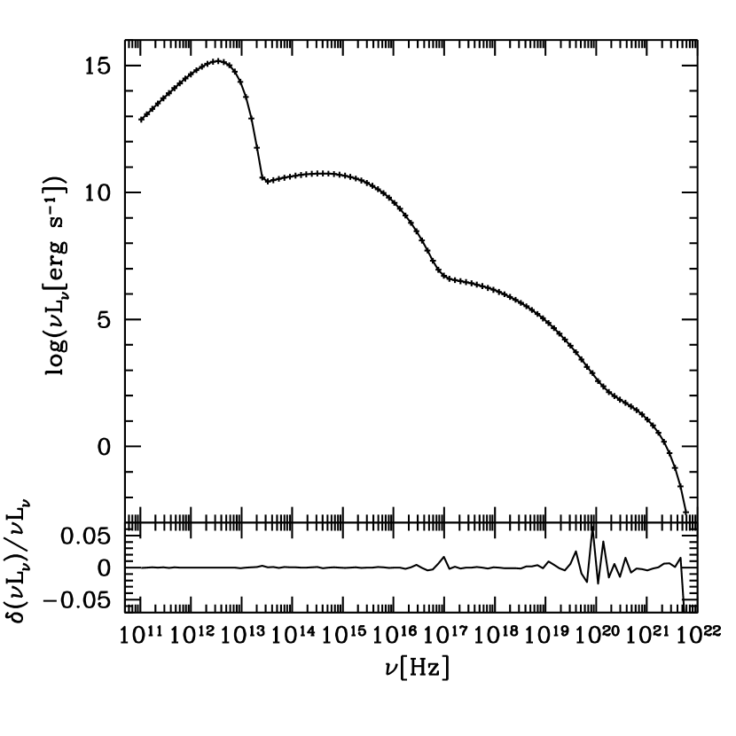
Figure 7: Spectra (upper panel) from grmonty (points) and sphere (solid line) produced by Comptonization of soft photons in a homogeneous, spherical cloud of hot plasma. Computations are done for: plasma optical thickness $\tau=10^{-4}$, plasma temperature $\Theta_{e}$=4 and the central source radiative temperature $kT_{r}/m_{e}c=10^{-8}$. Lower panel shows the fractional difference between the two spectra.

Figures 7, 8 and 9 show the radiation spectra (upper panels) produced by both codes and a fractional difference (bottom panels) between them for $\Theta_{e}=4$, $\Theta_{s}=10^{-8}$ and for various values of the optical depth $\tau$ = $10^{-4}$, 0.1, and 3. Figure 10 demonstrates that grmonty converges to the reference solution as $\propto N^{-1/2}$ for each optical depth.

7.4 Synchrotron self-absorbed spectra in black hole spacetimes

We consider two idealized problems: (1) smooth, spherically symmetric infall onto a Schwarzschild black hole; (2) a snapshot of a turbulent accretion flow around a Kerr black hole with $a/M=0.9375$ produced by general relativistic MHD simulation with the HARM code (Gammie et al., 2003). In this test, our reference solution is computed by the ray tracing code ibothros (Noble et al., 2007). ibothros solves the invariant form of the radiative transfer equation along geodesics that terminate in a fictitious camera at large distance. Spectra are constructed by imaging the source at successive frequencies and performing an angular integral over the images to estimate $\nu L_{\nu}$. In these tests scattering is turned off in grmonty.

There are algorithmic differences between grmonty and ibothros that lead to differences in their spectra.

First, grmonty measures the flux in energy and angular bins, whereas ibothros measures the flux at a particular inclination and energy. This is not an important effect unless there is sharp angular or energy structure in the spectrum.

The next difference is more subtle and is related to the treatment of gridded model data used to construct these tests. In grmonty  quantities such as the density, temperature, etc., are viewed as the average of these variables over a grid zone. In ibothros  the grid variables are viewed as zone-centered samples and a continuous distribution is created by multi-linear interpolation between zone centers. The difference is illustrated in one dimension in Figure 11. ibothros and grmonty therefore differ in zone-averaged emissivity by $O(\Delta x/L)^{2}$, where $\Delta x$ is the zone size and $L$ is the characteristic scale of the emitting structure.

Differences in the grmonty and ibothros spectra of structures with $\Delta x\ll L$ are therefore small. High frequency synchrotron emission, however, is exponentially dominated by emission from a few zones with highest $\nu_{s}$ (see equation (4b); these are the zones with highest temperature or strongest magnetic field). Then $\Delta x/L\sim 1$ for high frequency emission, and the grmonty and ibothros spectra differ by of order unity. A similar effect occurs for low frequency synchrotron emission where the optical depth is large. The spectrum is sensitive to the run of physical variables through the photosphere, which has size comparable to or smaller than a grid zone. The subsequent test results will omit these parts of the spectra. These inconsistencies between grmonty and ibothros could be eliminated by using identical, continuous models for subgrid reconstruction. But this would require significant investment in recoding that, in our view, is not worthwhile: to the extent that the spectrum depends on the flow structure at and below the grid scale, it is not reliable!

In spite of these differences, and other differences between the codes related to differing accuracy parameters, grmonty should converge on the ibothros result until the effects of data interpolation become the dominant sources of error.

Figures 12 and 13 show the spectrum and convergence relative to ibothros, respectively, for the spherical accretion problem. This problem is an attractive test for at least two reasons. First, the emission is isotropic so the effects of angular binning in grmonty are eliminated. Second, the flow is smooth, so the differences due to data interpolation will be small. Evidently the spherical accretion model converges at the expected, $N^{-1/2}$, rate.

Figures 14 and 15 show the spectrum and convergence relative to ibothros, respectively, for the turbulent accretion problem. This comparison is more challenging because the high energy emission originates in compact “hot spots.” Evidently the two models agree at the $10\%$ level everywhere, with the largest differences at high and low frequency, where the subgrid reconstruction comes into play. Excluding these high and low frequency regions, the agreement between the codes is at the few percent level.

8 Sample Calculation & Full Code Tests

We now apply grmonty to the same HARM simulation data used in the grmonty-ibothros comparison above, this time with scattering enabled. Figure 16 shows the resulting spectrum with the ibothros result shown for comparison. Evidently, scattering has little effect on the sub-mm spectrum since the scattering optical depth is small ($\sim 10^{-4}$) but the model now predicts a significant X-ray flux. A more detailed analysis of Comptonized spectra from GRMHD simulations in the context of Sgr A* will be given in a separate paper (Mościbrodzka et al., 2009).

Figure 17 shows the results of self-convergence tests for the full code. Convergence is initially slow but quickly approaches a rate proportional to $N^{-1/2}$ as spectral bins become sufficiently sampled. The spectra shown in Figure 16, which were taken from a single run with $10^{9}$ superphotons, were used for references.

9 Summary

We have described and tested a code that solves the radiative transfer problem for optically thin ionized plasmas in general spacetimes. The code treats the full angular dependence of emission and absorption, treats single Compton scattering exactly (double Compton and induced Compton scattering are neglected), and can be easily adapted to simulate emission from both analytic and numerical models. While we have specialized to synchrotron emission in this work, grmonty is constructed so that it is straightforward to include other relevant emission mechanisms such as bremsstrahlung with only minimal modification.

As a demonstration of a practical use for grmonty, we have computed the first spectra, including synchrotron emission and Compton scattering, from GRMHD models of a turbulent accretion disk. Other potential applications of our code are to neutron star accretion, emission from relativistic blast waves, and any problem where relativistic bulk motion makes radiation transfer treatments that expand the flow in orders of $v/c$ problematic.

Figure 1: Photon geodesics for isotropic emission from the rest frame of a fluid element in a marginally stable circular orbit around a Kerr black hole with $a/M=0.9375$. Results shown from grmonty (points) and geokerr (lines). The point size varies linearly with the z-coordinate.

Figure 2: Average fractional error in the conserved quantities $k_{t}$ and $k_{\phi}$ as a function of step size parameter $\varepsilon$. The solid line is $\varepsilon^{2}$, showing that grmonty’s geodesic integrator converges at second order.

Figure 3: In the top panel, the spectrum of a synchrotron emitting sphere with low optical depth above $\sim 10^{8}\textrm{ Hz}$ viewed nearly perpendicular to the magnetic field from grmonty (crosses) and from a semi-analytic procedure (solid line). The bottom panel shows the fractional difference between the two results.

Figure 4: Integrated fractional error in the grmonty spectrum for a synchrotron emitting sphere with low optical depth viewed nearly perpendicular to the magnetic field as a function of the number of superphotons produced. The results are similar for other magnetic field orientations. The dashed line is proportional to $N^{-1/2}$.

Figure 5: In the top panel, the spectrum of a synchrotron emitting sphere of high optical depth below $\sim 10^{11}\textrm{ Hz}$ viewed nearly perpendicular to the magnetic field from grmonty (crosses) and for a semi-analytic procedure (solid line). The bottom panel shows the fractional difference between the two results.

Figure 6: Integrated fractional error in the grmonty spectrum of a synchrotron emitting sphere with high optical depth as a function of the number of superphotons produced. The dashed line is proportional to $N^{-1/2}$.

Figure 8: Same as in Figure 7, but for $\tau$=0.1.

Figure 9: Same as in Figure 7, but for $\tau$=3.0.

Figure 10: Integrated fractional difference between grmonty and sphere for the spherical scattering test for optical depths of $10^{-4}$ (solid), $0.1$ (short dash), and $3$ (long dash). The dotted line shows the self-convergence results for the sphere code for an optical depth $\tau=10^{-4}$. The dot-dash line is proportional to $N^{-1/2}$.

Figure 11: Illustration of how interpolation can lead to a discrepancy between grmonty and ibothros when the spectrum is sensitive to grid-scale structure. Shown are the grid specified values for some fluid property (solid line), the interpolated values (dash line), and the average zone values based on interpolation (dotted line).

Figure 12: The top panel shows the spectrum of a radially infalling spherically symmetric source threaded with a radial magnetic field around a Schwarzschild black hole as computed by ibothros (solid line) and grmonty (crosses). The bottom panel shows the fractional difference between the two.

Figure 13: Integrated fractional error in the grmonty spectrum for the spherically symmetric Schwarzschild problem as a function of the number of superphotons produced. The dashed line is proportional to $N^{-1/2}$.

Figure 14: The top panel shows the spectrum of a snapshot from a HARM simulation of a turbulent accretion flow onto a Kerr black hole as computed by ibothros (solid line) and grmonty (crosses). The bottom panel shows the fractional difference between the two.

Figure 15: Integrated fractional error in the grmonty spectrum for the turbulent accretion problem as a function of the number of superphotons produced. The dashed line is proportional to $N^{-1/2}$.

Figure 16: Same as Figure 14 except Compton scattering is included. The histograms show the grmonty result for nearly edge-on and face-on inclinations and the solid line is the ibothros spectrum for a nearly edge-on inclination.

Figure 17: Self-convergence test results for the spectra shown in Figure 16. Convergence for the edge-on (solid) and face-on (dot-dash) spectra are shown. The dashed line is proportional to $N^{-1/2}$.

References

- Agol & Blaes (1996) Agol, E. & Blaes, O. 1996, MNRAS, 282, 965
- Bardeen et al. (1972) Bardeen, J. M., Press, W. H., Teukolsky, S. A. 1972, ApJ, 178, 347
- Beckwith & Done (2005) Beckwith, K. & Done, C. 2005, MNRAS, 359, 1217
- Böttcher & Liang (2001) Böttcher, M. & Liang, E. P. 2001, ApJ, 552, 248
- Böttcher et al. (2003) Böttcher, M., Jackson, D. R., & Liang, E. P. 2003, ApJ, 586, 389
- Canfield et al. (1987) Canfield, E., Howard, W. M. & Liang, E. P. 1987, ApJ, 323, 565
- Carrigan & Katz (1992) Carrigan, B. J. & Katz, J. I. 1992, ApJ, 399, 100
- Carter (1968) Carter, B. 1968, Phys. Rev., 174, 1559
- Coppi et al. (1993) Coppi, P., Blandford, R. D., & Rees, M. J. 1993, MNRAS, 262, 603
- Cullen (2001) Cullen, J. 2001, Journal of Computational Physics, 173, 175
- Dexter & Agol (2009) Dexter, J. & Agol, E. 2009, ApJ, 696, 1616
- Dove et al. (1997) Dove, J. B., Wilms, J., Begelman, M. C. 1997, ApJ, 487, 747
- Gammie et al. (2003) Gammie, C. F., McKinney, J. C., & Tóth, G. 2003, ApJ, 589, 444
- Górecki & Wilczewski (1984) Górecki, A. & Wilczewski, W. 1984, Acta Astron., 34, 141
- Hauschildt & Wehrse (1991) Hauschildt, P. H. & Wehrse, R. 1991, J. Quant. Rad. Spectrosc. Radiat. Transfer, 46, 81
- Hua (1997) Hua, X. M. 1997, ComPh, 11, 660
- Kahn (1950) Kahn, H. 1950, Nucleonics, 6, 5, 27
- Landau & Lifshitz (1975) Landau, L. D., Lifshitz, E. M. 1975, The Classical Theory of Fields, (Oxford: Pergamon)
- Laurent & Titarchuk (1999) Laurent, P. & Titarchuk, L. 1999, ApJ, 511, 289
- Leung et al. (2009) Leung, P. K. & Gammie, C. F., in prep
- Mihalas & Mihalas (1984) Mihalas, D., & Mihalas, B. W. 1984, Foundations of Radiation Hydrodynamics, (New York: Oxford Univ. Press)
- Molnar & Birkinshaw (1999) Molnar, S. M., & Birkinshaw, M. 1999, ApJ, 523, 78
- Mościbrodzka et al. (2009) Mościbrodzka, M., Gammie, C. F., Dolence, J., Shiokawa, H., & Leung, P. K., in prep
- Noble et al. (2007) Noble, S. C., Leung, P. K., Gammie, C. F., & Book, L. G. 2007, CQG, 24, 259
- Poutanen & Svensson (1996) Poutanen, J. & Svensson, R. 1996, ApJ, 470, 249
- Pozdynakov et al. (1983) Pozdynakov, L. A., Sobol, I. M., & Syunyaev, R. A. 1983, ASPRv, 2, 189
- Rauch & Blandford (1994) Rauch, K. P. & Blandford, R. D. 1994, ApJ, 421, 46
- Schnittman (2006) Schnittman, J. D. 2006, Ph.D. thesis, Massachusetts Institute of Technology
- Schnittman & Krolik (2009) Schnittman, J. D. & Krolik, J. H. 2009, preprint (astro-ph/09023982)
- Schnittman et al. (2006) Schnittman, J. D., Krolik, J. H., & Hawley, J. F. 2006, ApJ, 651, 1031
- Stern et al. (1995) Stern, B. E., Begelman, M. C., Sikora, M., & Svensson, R. 1995, MNRAS, 272, 291
- Wu et al. (2008) Wu, K., Fuerst, S. V., Mizuno, Y., Nishikawa, K.-I., Branduardi-Raymont, G., & Lee, K.-G. 2008, ChJAS, 8, 226
- Yao et al. (2005) Yao, Y., Zhang, S. N., Zhang, X., Feng, Y., & Robinson, C. R. 2005, ApJ, 619, 446
- Zane et al. (1996) Zane, S., Turolla, R., Nobili, L., & Erna, M. 1996, ApJ, 466, 871