Maximally informative pairwise interactions in networks

Abstract

Several types of biological networks have recently been shown to be accurately described by a maximum entropy model with pairwise interactions, also known as the Ising model. Here we present an approach for finding the optimal mappings between input signals and network states that allow the network to convey the maximal information about input signals drawn from a given distribution. This mapping also produces a set of linear equations for calculating the optimal Ising model coupling constants, as well as geometric properties that indicate the applicability of the pairwise Ising model. We show that the optimal pairwise interactions are on average zero for Gaussian and uniformly distributed inputs, whereas they are non-zero for inputs approximating those in natural environments. These non-zero network interactions are predicted to increase in strength as the noise in the response functions of each network node increases. This approach also suggests ways for how interactions with unmeasured parts of the network can be inferred from the parameters of response functions for the measured network nodes.

I Introduction

Many organisms rely on complex biological networks both within and between cells to process information about their environments Bray (1995); Bock and Goode (2001). As such, their performance can be quantified using the tools of information theory Cover and Thomas (1991); Tkačik et al. (2008); Tostevin and ten Wolde (2009); Ziv et al. (2007). Because these networks often involve large numbers of nodes, one might fear that difficult-to-measure high-order interactions are important for their function. Surprisingly, recent studies have shown that neural networks Schneidman et al. (2006); Shlens et al. (2006); Tang et al. (2008); Pillow et al. (2008), gene regulatory networks Lezon et al. (2006); Walczak and Wolynes (2009), and protein sequences Socolich et al. (2005); Bialek and Ranganathan (2007) can be accurately described by a maximum entropy model including only up to second-order interactions. In these studies the nodes of biological networks are approximated as existing in one of a finite number of discrete states at any given time. In a gene regulatory network the individual genes are binary variables, being either in the inactivated or the metabolically expensive activated states. Similarly, in a protein the nodes are the amino acid sites on a chain which can take on any one of twenty values.

We will work in the context of neural networks, where the neurons communicate by firing voltage pulses commonly referred to as spikes Rieke et al. (1997). When considered in small enough time windows, the state of a network of $N$ neurons can be represented by a binary word $\sigma=\left(\sigma_{1},\sigma_{2},\ldots,\sigma_{N}\right)$, where the state of neuron i is given by $\sigma_{i}=1$ if it is spiking and $\sigma_{i}=-1$ if it is silent, similar to the $\uparrow$/$\downarrow$ states of Ising spins.

The Ising model, developed in statistical physics to describe pairwise interactions between spins, can also be used to describe the state probabilities $P_{\sigma}$ of a neural network:

$$P_{\sigma}=\dfrac{1}{Z}\textrm{exp}\left[\displaystyle\sum_{i}h_{i}\sigma_{i}+\displaystyle\sum_{i\neq j}J_{ij}\sigma_{i}\sigma_{j}\right].$$ (1)

Here, $Z$ is the partition function and the parameters $\left\{h_{i}\right\}$ and $\left\{J_{ij}\right\}$ are the coupling constants. This is the least structured (or equivalently, the maximum entropy Jaynes (1957)) model consistent with given first- and second-order correlations, obtained by measuring $\left\langle\sigma_{i}\right\rangle$ and $\left\langle\sigma_{i}\sigma_{j}\right\rangle$, where these averages are over the distribution of network states.

In magnetic systems one seeks the response probabilities from the coupling constants, but in the case of neural networks one seeks to solve the inverse problem of determining the coupling constants from measurements of the state probabilities. Because this model provides a concise and accurate description of response patterns in networks of real neurons Schneidman et al. (2006); Shlens et al. (2006); Tang et al. (2008); Pillow et al. (2008), we are interested in finding the values of the coupling constants which allow neural responses to convey the maximum amount of information about input signals.

The Shannon mutual information can be written as the difference between the so-called response and noise entropies Cover and Thomas (1991):

$$I=H_{\rm{resp}}-H_{\rm{noise}}.$$

The response entropy quantifies the diversity of network responses across all possible input signals $\{\mathcal{I}\}$. For our discrete neural system this is given by

$$H_{\rm{resp}}=-\displaystyle\sum_{\left\{\sigma\right\}}P_{\sigma}\log_{2}\left(P_{\sigma}\right).$$ (2)

In the absence of any constraints on the neural responses, $H_{\rm{resp}}$ is maximized when all $2^{N}$ states are equally likely Attwell and Laughlin (2001).

The noise entropy takes into account that the network states may vary with respect to repeated presentations of inputs, which reduces the amount of information transmitted. The noise entropy is obtained by computing the conditional response entropy $P_{\sigma|{\mathcal{I}}}$, and averaging over all inputs,

$$H_{\rm{noise}}=-\displaystyle\int d\mathcal{I}~{}P_{\mathcal{I}}\displaystyle\sum_{\left\{\sigma\right\}}P_{\sigma|{\mathcal{I}}}\log_{2}\left(P_{\sigma|{\mathcal{I}}}\right),$$ (3)

where $P_{\mathcal{I}}$ is the input probability distribution. Thus in order to find the maximally informative coupling constants, we must first confront the difficult problem of finding the optimal mapping between inputs $\mathcal{I}$ and network states $\sigma$.

II Decision boundaries

The simplest mappings from inputs to neural response involve only a single input dimension de Boer and Kuyper (1968); Meister and Berry (1999); Schwartz et al. (2006); Victor and Shapley (1980). In such cases, the response of a single neuron can often be described by a sigmoidal function with respect to the relevant input dimension Rieke et al. (1997); Laughlin (1981). However, studies in various sensory systems, including the retina Fairhall et al. (2006), the primary visual Rust et al. (2005); Chen et al. (2007); Touryan et al. (2002); Felsen et al. (2005), auditory Atencio et al. (2008), and somatosensory Maravall et al. (2007) cortices, have shown that neural response can be affected by multiple input components, resulting in highly nonlinear, multi-dimensional mappings from input signals to neural responses.

In Fig. 1 we provide examples of response functions estimated for two neurons in the cat primary visual cortex Sharpee et al. (2006). For each neuron, the heat map shows the average firing rate in the space of the two most relevant input dimensions. As this figure illustrates, even in two dimensions the mapping from inputs to the neural response (in this case the presence or absence of a spike in a small time bin) can be quite complex. Nevertheless, one can delineate regions in the input space where the firing rate is above or below its average (red solid lines). As an approximation, one can equate all firing rate values to the maximum value in regions where it is above average, and to zero in regions where it is below average. This approximation of a sharp transition region of the response function is equivalent to assuming small noise in the response. Across the boundary separating these regions, we will assume that the firing rate varies from zero to the maximum in a smooth manner (inset in Fig. 2).

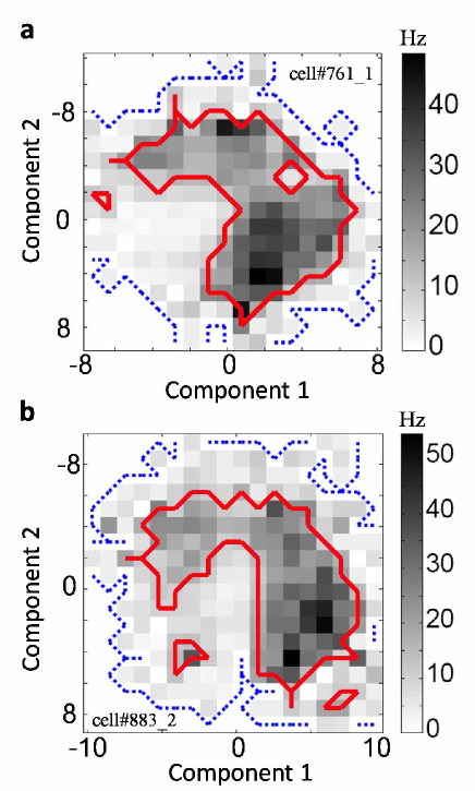
Figure 1: (Color online) Example analysis of firing rate for a simple, a, and a complex, b, cell in the cat primary visual cortex probed with natural stimuli from the dataset Sharpee et al. (2006). Two relevant input dimensions were found for each neuron using the maximally informative dimensions method described in Sharpee et al. (2004). Color shows the firing rate as a function of input similarity to the first (x-axis) and second (y-axis) relevant input dimensions. The values on the x- and y- axis have been normalized to have zero mean and unit variance. Blue (dashed) lines show regions with signal-to-noise ratio $>$ 2.0. Red (solid) lines are drawn at half the maximum rate and represent estimates of the decision boundaries.

As we discuss below, this approximation simplifies the response functions enough to make the optimization problem tractable, yet it still allows for a large diversity of nonlinear dependencies. Upon discretization into a binary variable, the firing rate of a single neuron can be described by specifying regions in the input space where spiking or silence is nearly always observed. We will assume that these deterministic regions are connected by sigmoidal transition regions called decision boundaries Sharpee and Bialek (2007), near which $P_{\sigma|\mathcal{I}}\approx 0.5$. The crucial component in the model is that the sigmoidal transitions are sharp, affecting only a small portion of the input space. Quantitatively, decision boundaries are well defined if the width of the sigmoidal transition region is much smaller than the radius of curvature of the boundary.

The decision boundary approach is amenable to the calculation of mutual information. The contribution to the noise entropy $H_{\textrm{noise}}$ from inputs near the boundary is on the order of one bit and decays to zero in the spiking/silent regions (Fig. 2). We introduce a weighting factor $\eta$ to denote the summed contribution of inputs near a decision boundary obtained by integrating $-\displaystyle\sum_{\sigma}P_{\sigma|x}\log_{2}\left(P_{\sigma|x}\right)$ across the boundary. The factor $\eta$ depends on the specific functional form of the transition from spiking to silence, and represents a measure of neuronal noise. In a single-neuron system, the total noise entropy is then an integral along the boundary, $H_{\rm{noise}}\approx\eta~{}\int_{\gamma}ds~{}P_{\mathcal{I}}$, where $\gamma$ represents the boundary, and the response entropy is $H_{\rm{resp}}=-P\log_{2}P-\left(1-P\right)\log_{2}\left(1-P\right)$, where $P$ is the spike probability of the neuron, equal to the integral of $P_{\mathcal{I}}$ over the spiking region.

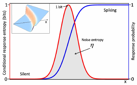
Figure 2: (Color online) Schematic of response probability and noise entropy. The response function in two dimensions (inset) is assumed to be deterministic everywhere except at the transition region which may curve in the input space. In a direction x, perpendicular to some point on the decision boundary, the response function is sigmoidal (blue, no shading) going from silent to spiking. The conditional response entropy (red, shading underneath) is $-P_{\rm{spike}|\rm{x}}\log_{2}\left(P_{\rm{spike}|\rm{x}}\right)-\left(1-P_{\rm{spike}|\rm{x}}\right)\log_{2}\left(1-P_{\rm{spike}|\rm{x}}\right)$ and decays to zero at $x=\pm\infty$. The contribution to the total noise entropy due to this cross-section, $\eta$, is the shaded area under the conditional response entropy curve.

The decision boundary approach is also easily extended to the case of multiple neurons, as shown in Fig. 3(a). In the multi-neuronal circuit, the various response patterns are obtained from intersections between decision boundaries of individual neurons. In principle, all $2^{N}$ response patterns can be obtained in this way. We denote as $G_{\sigma}$ the region of the space where inputs elicit a response $\sigma$ from the network. To calculate the response entropy for a given set of decision boundaries in a $D-$dimensional space, the state probabilities are evaluated as $D-$dimensional integrals over $\{G_{\sigma}\}$

$$P_{\sigma}=\displaystyle\int\limits_{G_{\sigma}}d^{D}\textbf{r}P_{\mathcal{I}}\left(\textbf{r}\right),$$ (4)

weighted by $P_{\mathcal{I}}$. Just as in the case of a single neuron, the network response is assumed to be deterministic everywhere except near any of the transition regions. Near a decision boundary, the network can be with approximately equal probability in one of two states that differ in the response of the neuron associated with that boundary. Thus, such inputs contribute $\sim 1$ bit to the noise entropy, cf. Eq. (3) and Fig. 2. The total noise entropy can therefore be approximated as a surface integral over all decision boundaries weighted by $P_{\mathcal{I}}$,

$$H_{\rm{noise}}\approx\eta\displaystyle\sum_{n=1}^{N}~{}\displaystyle\int\limits_{\gamma_{n}}ds~{}P_{\mathcal{I}},$$ (5)

where $\gamma_{n}$ is the decision boundary of the $n^{\text{th}}$ neuron. In this paper we will assume that $\eta$ is the same for all neurons and is position-independent, but the extension to the more general case of spatially varying $\eta$ is possible Sharpee and Bialek (2007). Finding the optimal mapping from inputs to network states can now be turned into a variational problem with respect to decision boundaries shapes and locations.

III Results

III.1 General solution for optimal coupling constants

Our approach for finding the optimal coupling constants consists of three steps. The first step is to find the optimal mapping from inputs to network states, as described by decision boundaries. The second step is to use this mapping to compute the optimal values of the response probabilities by averaging across all possible inputs. The final step is to determine the coupling constants of the Ising model from the set of optimal response probabilities.

Due to a high metabolic cost of spiking, we are interested in finding the optimal mapping from inputs to network states that result in a certain average spike probability across all neurons:

$$P=\dfrac{1}{N}\displaystyle\sum_{\sigma}S_{\sigma}P_{\sigma},$$ (6)

where $S_{\sigma}$ is the number of “up spins”, or firing neurons, in configuration $\sigma$. Taking metabolic constraints into account, we maximize the functional

$$F = H_{\rm{resp}}-H_{\rm{noise}}-\lambda\left(NP-\displaystyle\sum_{n=1}^{N}P_{n}\right)$$ (7)

$$-\displaystyle\sum_{\sigma}\beta_{\sigma}\left(P_{\sigma}-\displaystyle\int\limits_{G_{\sigma}}d^{D}\textbf{r}P_{\mathcal{I}}\left(\textbf{r}\right)\right)$$

where $\lambda$, $\left\{\beta_{\sigma}\right\}$ are Lagrange multipliers for the constraints and the last term demands self-consistency through Eq. (4).

To accomplish the first step, we optimize the shape of each segment between two intersection points. Requiring $\frac{\delta F}{\delta\bf{r}}=0$ yields the following equation

$$\eta\left[\kappa+\hat{\textbf{n}}\cdot\nabla P_{\mathcal{I}}\left(\textbf{r}\right)\right]+\beta_{\sigma_{1},...,\sigma_{i-1},\uparrow,\sigma_{i+1},...,\sigma_{N}}$$

$$-\beta_{\sigma_{1},...,\sigma_{i-1},\downarrow,\sigma_{i+1},...,\sigma_{N}}=0,$$ (8)

for the segment of the $i^{th}$ decision boundary that separates the regions $G_{\sigma_{1},...,\sigma_{i-1},\uparrow,\sigma_{i+1},...,\sigma_{N}}$ and $G_{\sigma_{1},...,\sigma_{i-1},\downarrow,\sigma_{i+1},...,\sigma_{N}}$. Here, $\hat{\textbf{n}}$ is the unit normal vector to the decision boundary, and $\kappa=\nabla\cdot\hat{\textbf{n}}$ is the total curvature of the boundary. We then optimize with respect to the state probabilities, $\frac{\delta F}{\delta P_{\sigma}}=0$, which gives a set of equations

$$\beta_{\sigma}=S_{\sigma}\lambda-\dfrac{1}{\rm{ln}2}\left(1+\textrm{ln}P_{\sigma}\right).$$ (9)

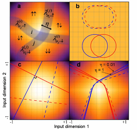
Figure 3: (Color online) Network decision boundaries. Color in input space corresponds to the input distribution $P_{\mathcal{I}}$ and each line is a boundary for an individual neuron. a, For a general intersection between neurons $i$ and $j$, the boundaries divide the space into four regions corresponding to the possible network states (e.g. $G_{\sigma_{i}=\uparrow,\sigma_{j}=\uparrow}$). Each segment has a width $\eta$ which determines the noise level, and is described by a parameter $\lambda^{\left(i\right)}_{\sigma^{\prime}}$, cf. Eq. (10). b, In a uniform space, with two neurons (different colors/shading), the boundary segments satisfying the optimality condition are circular. Networks which have segments with different curvatures (dashed) are less informative than smooth circles (solid). c, In a Gaussian space (in units of standard deviations), straight perpendicular lines (solid) provide more information about inputs than decision boundaries that intersect at any other angle (dashed). d, For approximately natural inputs (plotted in units of standard deviations), the suboptimal balanced solutions (dashed) are two independent boundaries with the same $P$. The optimal solutions (solid) change their curvature at the intersection point, and depend on the neuronal noise level $\eta$.

Combining Eqs. (8) and (9), we arrive at the following equation for the segment of the $i^{th}$ decision boundary across which $\sigma_{i}$ changes while leaving the rest of the network in state $\sigma^{\prime}$:

$$\lambda^{\left(i\right)}_{\sigma^{\prime}}+\kappa+\hat{\textbf{n}}\cdot\nabla P_{\mathcal{I}}\left(\textbf{r}\right)=0.$$ (10)

The parameter

$$\lambda^{\left(i\right)}_{\sigma^{\prime}}=\dfrac{1}{\eta}\left[\lambda-\textrm{log}_{2}\left(\dfrac{P_{\sigma_{1},...,\sigma_{i-1},\uparrow,\sigma_{i+1},...,\sigma_{N}}}{P_{\sigma_{1},...,\sigma_{i-1},\downarrow,\sigma_{i+1},...,\sigma_{N}}}\right)\right],$$ (11)

is specific to that segment, and is determined by the ratio of probabilities of observing the states which this segment separates. Generally, this ratio (and therefore the parameter $\lambda^{\left(i\right)}_{\sigma^{\prime}}$) may change when the boundaries intersect. For example, in the schematic in Fig. 3(a), $\lambda^{\left(i\right)}_{\sigma_{j}=\downarrow}$ depends on the ratio of $P_{\sigma_{i}=\uparrow,\sigma_{j}=\downarrow}/P_{\sigma_{i}=\downarrow,\sigma_{j}=\downarrow}$, whereas $\lambda^{\left(i\right)}_{\sigma_{j}=\uparrow}$ depends on $P_{\sigma_{i}=\uparrow,\sigma_{j}=\uparrow}/P_{\sigma_{i}=\downarrow,\sigma_{j}=\uparrow}$. The values of the parameters for the two segments of the $i^{th}$ boundary are equal only when $P_{\sigma_{i}=\uparrow,\sigma_{j}=\downarrow}/P_{\sigma_{i}=\downarrow,\sigma_{j}=\downarrow}=P_{\sigma_{i}=\uparrow,\sigma_{j}=\uparrow}/P_{\sigma_{i}=\downarrow,\sigma_{j}=\uparrow}$. This condition is satisfied when the neurons are independent. Therefore, we will refer to the special case of a solution where $\lambda$ does not change its value across any intersection points as an independent boundary. In fact, Eq. (10) with a constant $\lambda$ is the same as was obtained in Sharpee and Bialek (2007) for a network with only one neuron. In that case, the boundary was described by a single parameter $\lambda$, which was determined from the neuron’s firing rate. Thus, in the case of multiple neurons, the individual decision boundaries are concatenations of segments of optimal boundaries computed for single neurons with, in general different, constraints. A change in $\lambda_{\sigma^{\prime}}^{(i)}$ across an intersection point results in a kink – an abrupt change in the curvature of the boundary. Thus, by measuring the change in curvature of a decision boundary of an individual neuron one can obtain indirect measurements on the degree of interdependence with other, possibly unmeasured, neurons.

Our main observation is that the $\lambda$-parameters determining decision boundary segments can be directly related to the coupling constants of the Ising model through a set of linear relationships. For example, consider two neurons $i$ and $j$ within a network of $N$ neurons whose decision boundaries intersect. It follows from Eq. (11) that the change in $\lambda$-parameters along a decision boundary is the same for the $i$th and $j$th neuron, and is given by:

$$\lambda^{\left(i\right)}_{\sigma_{j}=\uparrow}-\lambda^{\left(i\right)}_{\sigma_{j}=\downarrow}=\lambda^{\left(j\right)}_{\sigma_{i}=\uparrow}-\lambda^{\left(j\right)}_{\sigma_{i}=\downarrow}=$$

$$=\frac{1}{\eta}~{}\textrm{log}_{2}\left[\frac{P_{\sigma^{\prime\prime},\sigma_{i}=\downarrow,\sigma_{j}=\downarrow}P_{\sigma^{\prime\prime},\sigma_{i}=\uparrow,\sigma_{j}=\uparrow}}{P_{\sigma^{\prime\prime},\sigma_{i}=\uparrow,\sigma_{j}=\downarrow}P_{\sigma^{\prime\prime},\sigma_{i}=\downarrow,\sigma_{j}=\uparrow}}\right].$$ (12)

where $\sigma^{\prime\prime}$ represents the network state of all the neurons other than $i$ and $j$. Taking into account the Ising model via Eq. (1), this leads to a simple relationship for the interaction terms $\left\{J_{ij}\right\}$:

$$\lambda^{\left(i\right)}_{\sigma_{j}=\uparrow}-\lambda^{\left(i\right)}_{\sigma_{j}=\downarrow}=\lambda^{\left(j\right)}_{\sigma_{i}=\uparrow}-\lambda^{\left(j\right)}_{\sigma_{i}=\downarrow}=-\dfrac{2\left(J_{ij}+J_{ji}\right)}{\eta\ln 2}.$$ (13)

We note that only the average (“symmetric”) component of pairwise interactions can be determined in the Ising model. Indeed, simultaneously increasing $J_{ij}$ and decreasing $J_{ji}$ by the same amount will leave the Ising model probabilities unchanged because of the perturbation symmetry in Eq. (1). This same limitation is present in the determination of $\left\{J_{ij}\right\}$ via any method (e.g. an inverse Ising algorithm).

Once the interaction terms $\left\{J_{ij}\right\}$ are known, the local fields can be found as well from Eq. (11):

$$\lambda_{{\sigma}^{\prime}}^{(i)}-\frac{\lambda}{\eta}=-\frac{2}{\eta\ln 2}\left[h_{i}+\sum_{k\neq i}J_{ik}\sigma_{k}\right].$$ (14)

This equation can be evaluated for any response pattern $\sigma^{\prime}$, because consistency between changes in $\lambda$ is guaranteed by Eq. (13).

The linear relationships between the Ising model coupling constants and the $\{\lambda^{\left(i\right)}_{\sigma^{\prime}}\}$ parameters are useful, because they can indicate what configurations of network decision boundaries can be consistent with an Ising model. First, Eq. (13) tells us that if the $i^{\rm{th}}$ boundary is smooth at an intersection with another boundary $j$, then the average pairwise interaction in the Ising model between neurons $i$ and $j$ is zero [as mentioned above the cases of truly zero interaction $J_{ij}=J_{ji}=0$ and that of a balanced coupling $J_{ij}=-J_{ji}$ cannot be distinguished in an Ising model]. Second, we know that if one boundary is smooth at an intersection, then any other boundary it intersects with is also smooth at that point. More generally, the change in curvature has to be the same for the two boundaries and we can use it to determine the average pairwise interaction between the two neurons. A third point is that the change in curvature has to be the same at all points where the same two boundaries intersect. For example, intersection between two planar boundaries is allowed because the change is curvature is zero at points across the intersection line. In cases where intersections form disjoint sets the equal change in curvature would presumably have to be due to a symmetry of decision boundaries.

In summary then, we have the analytical equations for the maximally informative decision boundaries of a network, through Eqs. (10) and (11). We now study their solutions for specific input distributions and then determine, through Eqs. (13) and (14), the corresponding maximally informative coupling constants.

III.2 Uniform and Gaussian distributions

We first consider the cases of uniformly and Gaussian distributed input signals. As discussed above, finding optimal configurations of decision boundaries is a trade-off between maximizing the response entropy and minimizing the noise entropy. Segments of decision boundaries described by Eq. (10) minimize the noise entropy locally, whereas changes in the $\lambda$ parameters arise as a result of maximizing the response entropy. The independent decision boundaries, which have one constant $\lambda$ for each boundary, minimize the noise entropy globally for a given firing rate. Because for one neuron, specifying the spike probability is sufficient to determine the response entropy $P_{1}=P$, cf. Eq. (6), and $H_{\textrm{resp}}=-P\log_{2}P-\left(1-P\right)\log_{2}\left(1-P\right)$, maximizing information for a given spike probability is equivalent to minimizing the noise entropy Sharpee and Bialek (2007). When finding the optimal configuration of boundaries in a network with an arbitrary number of nodes, the response entropy is not fixed, because the response probability may vary for each node (it is specified only on average across the network). However, if there is some way of arranging a collection of independent boundaries to obtain response probabilities that also maximize the response entropy, then such a configuration must be optimal because it simultaneously minimizes the noise entropy and maximizes the response entropy. It turns out that such solutions are possible for both the uniformly and Gaussian distributed input signals.

For the simple case of two neurons receiving a two-dimensional uniformly distributed input, as in Fig. 3(b), the optimal independent boundaries are circles, because they minimize the noise entropy (circumference) for a given probability $P$ (area). In general, the response entropy, Eq. (2), is maximized for the case of two neurons when the probability of both neurons spiking is equal to $P^{2}$. It is always possible to arrange two circular boundaries to satisfy this requirement. The same reasoning extends to overlapping hyperspheres in higher dimensions, allowing one to calculate the optimal network decision boundary configuration for uniform inputs. Therefore, for uniformly distributed inputs the optimal network decision boundaries are overlapping circles in two dimensions or hyperspheres in higher dimensions.

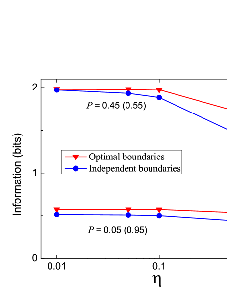
Figure 4: (Color online) Information from independent and optimally coupled network boundaries as a function of neuronal noise level. In both examples shown here, the independent boundaries (blue circles) lose information faster than the optimal boundaries (red triangles) as the noise level $\eta$ increases. Each curve represents two response probabilities (e.g. $P=$ 0.45 and 0.55) because information is invariant under switching the spiking/silent regions.

For an uncorrelated Gaussian distribution, Fig. 3(c), the independent boundaries are $\left(D-1\right)$-dimensional hyperplanes Sharpee and Bialek (2007). If we again consider two neurons in a two-dimensional input space, then the individual response probabilities for each boundary determine the perpendicular distance from the origin to the lines. Any two straight lines will have the same noise entropy, independent of the angle between them. However, orthogonal lines (orthogonal hyperplanes in higher dimensions) maximize the response entropy. The optimality of orthogonal boundaries holds for any number of neurons and any input dimensionality. We also find that for a given average firing rate across the network, the maximal information per neuron does not depend on input dimensionality as long as the number of neurons $N$ is less than the input dimensionality $D$. For $N>D$, the information per neuron begins to decrease with $N$, indicating redundancy between neurons.

III.3 Naturalistic distributions

Biological organisms rarely experience uniform or Gaussian input distributions in their natural environments and might be evolutionarily optimized to optimally process inputs with very different statistics. To approximate natural inputs, we use a two-dimensional Laplace distribution, $P_{\mathcal{I}}\left(\textbf{r}\right)\propto\textrm{exp}\left(-|x|-|y|\right)$, which captures the large-amplitude fluctuations observed in natural stimuli Ruderman and Bialek (1994); Simoncelli and Olshausen (2001), as well as bursting in protein concentrations within a cell Paulsson (2004). For this input distribution there are four families of solutions to Eq. (10) (see Sharpee and Bialek (2007) for details), giving rise to many potentially optimal network boundaries. For a given $\lambda$, the decision boundaries can be found analytically. To find the appropriate value of the $\lambda$’s, we numerically solved Eq. (10) using Mathematica mat (2007). We found no solutions for independent boundaries. The optimal boundaries therefore will have different $\lambda$’s, and kinks at intersection points. As a result, the neurons will have a nonzero average coupling between them, examples of which are shown in Fig. 3(d).

We found that the shapes of the boundaries change with the noise level $\eta$, which does not happen for independent boundaries Sharpee and Bialek (2007). To see if this noise dependence gives the network the ability to compensate for noise in some way, we look at the maximum possible information the optimal network boundaries are able to encode about this particular input distribution for different noise levels (Fig. 4). We compare this to the suboptimal combination of two independent boundaries with the same $P$. The figure illustrates that the optimal solutions decrease in information less quickly as the noise level increases. The improvement in performance results from their ability to change shape in order to compensate for the increasing noise level.

We calculated both $h\equiv h_{1}=h_{2}$ and $J\equiv\left(J_{12}+J_{21}\right)/2$ for various noise levels and response probabilities. Fig. 5(a) and (c) show the local field $h$ is practically independent of the noise level but does depend on the response probability. The coupling strength, however, depends on both noise level and response probability, increasing in magnitude with neuronal noise, shown in Fig. 5(b). The combination of this result and the noise compensation observed in Fig. 4, suggests that the network is able to use pairwise coupling for error correction, with larger noise requiring larger coupling strengths. This strategy is similar to the adage “two heads are better than one”, to which we add “$\ldots$ especially if the two heads are noisy”.

In Fig. 5(d) we observe that the sign of the coupling changes as the value of $P$ crosses $1/2$. When $P=1/2$, the optimal solution is an X crossing through the origin, which is the only response probability for which the network boundary is made of two independent boundaries, making $J=0$ for any noise level when $P=1/2$. It can also be seen that $J\rightarrow 0$ as $\eta\rightarrow 0$ for $P\neq 1/2$. Curiously, for a given $\eta$, the dependence of the optimal $J$ on $P$ is highly nonmonotonic: it changes sign across $P=1/2$, and reaches a maximum(minimum) value for $P\approx 0.25(0.75)$.

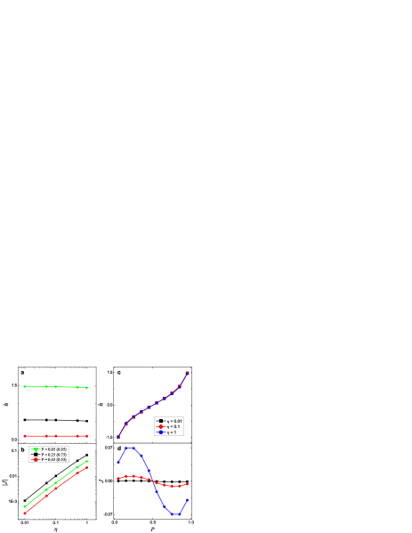
Figure 5: (Color online) Optimal coupling constants for naturalistic inputs. a, The local fields show very little dependence on the noise level of the neurons, but the magnitude of the interaction strength $J$, b, increases in the same fashion with the noise level regardless of the response probability $P$. c, $h$ depends strongly on the response probability. d, $J$ changes sign about $P=1/2$. Below this point the coupling is excitatory, and above it the coupling is inhibitory.

IV Discussion

The general mapping between inputs and maximally informative network responses in the decision boundary approximation has allowed us to calculate the Ising model coupling constants. In this approach, network responses to a given input are not described by an Ising model, which emerges after averaging network responses across many different inputs. Although there are many configurations of network decision boundaries that can be consistent with a pairwise-interaction model, certain restrictions apply. For example, the change in curvature of a decision boundary that can occur when two boundaries intersect has to be the same for both boundaries, and, if they intersect at more than one disjoint surfaces then the curvatures of those surfaces must be the same.

We find that for both the uniform and Gaussian input distributions the optimal network boundaries are independent. This implies that the average interaction strength is zero for all pairs of nodes through Eq. (13). Such balance between excitatory and inhibitory connections has been observed in other contexts including rapid state switching Tsodyks and Sejnowski (1995), Hebbian learning Song et al. (2000), and selective amplification Murphy and Miller (2009). In this context balanced coupling is just one possible configuration of a network of decision boundaries and happens to be optimal for uniformly and Gaussian distributed inputs.

For a more realistic input distribution, the Laplace distribution, we found the optimal boundaries were not smooth at intersection points. This indicates that the average coupling between the nodes in the network should be non-zero to achieve maximal information transmission. We also observed that the optimal configuration of the network depended on the noise level in the responses of the nodes, giving the network the ability to partially compensate for the encoding errors introduced by the noise, which did not happen for the less natural input distributions considered. Also, the fact that $J$ can be positive or negative between two nodes leads to the potential for many stable states in the network, which could give the network the capacity to function as autoassociative memory, as in the Hopfield model Hopfield (1982); Amit et al. (1985). Similar network behaviors were reported in Prentice et al. (2009) for networks of ten neurons, where the optimal coupling constants were numerically found for correlated binary and Gaussian inputs. Our approach is different in that we use an Ising model to describe average network responses, but not responses to particular inputs, $P_{\sigma|\mathcal{I}}$.

Previous experiments have shown that simultaneous recordings from neural populations could be well described by the Ising model. In one such experiment using natural inputs Schneidman et al. (2006), the distributions of coupling constants showed an average $h$ which was of order unity and negative and average $J$ which was small and positive. Our results for the Laplace distribution are in qualitative agreement with these previous findings if one assumes a response probability $P<1/2$. Due to the high metabolic cost of spiking, this is a plausible assumption to make.

The method we have put forth goes beyond predicting the maximally informative coupling constants, to make statements about optimal coding strategies for networks. Although both uniform and Gaussian inputs can be optimally encoded by balanced networks, for example, their organizational strategies are remarkably different. In the uniform input case, the optimal boundaries curve in all dimensions, meaning each node is attending to and encoding information about every component of the possibly high-dimensional input, and they organize themselves by determining the optimal amount of overlap between boundaries. However, for the Gaussian distribution, each boundary is planar, indicating that the nodes of the network are sensitive to only one component of the input. The optimal strategy for networks receiving this type of input is to attend to and encode orthogonal directions in the input space, minimizing the redundancy in the coding process.

In terms of practical applications, perhaps the most useful aspect of this framework is the ability to infer the strength of pairwise interactions with other nodes in the network by examining decision boundaries of single nodes, cf. Eq. (13).

The observation of different types of pairwise interactions for networks processing Gaussian and naturalistic Laplace inputs raises the possibility of discovering novel adaptive phenomena. Previous studies in several sensory modalities have demonstrated that the principle of information maximization can account well for changes in the relevant input dimensions Smirnakis et al. (1997); Shapley and Victor (1978); Kim and Rieke (2001); Srinivasan et al. (1982); Buchsbaum and Gottschalk (1983); Shapley and Victor (1979); Chander and Chichilnisky (2001); Hosoya et al. (2005); Sharpee et al. (2006); Theunissen et al. (2000); Nagel and Doupe (2006a); David et al. (2004) as well as the neural gain Laughlin (1981); Brenner et al. (2000); Fairhall et al. (2001); Nagel and Doupe (2006a) following changes in the input distribution. For example, nonlinear gain functions have been shown to rescale with changes in input variance Shapley and Victor (1979); Brenner et al. (2000); Fairhall et al. (2001); Maravall et al. (2007); Nagel and Doupe (2006b). Our results suggest that if neurons were adapted on one hand to Gaussian inputs, and then to naturalistic non-Gaussian inputs, then multi-dimensional input/output functions of individual neurons might change qualitatively, with larger changes expected for noisier neurons.

By studying the geometry of interacting decision boundaries we have gained insights into optimal coding strategies and coupling mechanisms in networks. Our work focused on the application to neural networks, but the method developed here is general to any network with nodes which have multidimensional, sigmoidal response functions. Although we have only considered three particular distributions of inputs, the framework described here is general and can be applied to other classes of inputs with the potential of uncovering novel, metabolically efficient combinatorial coding schemes. In addition to making predictions for how optimal pairwise interactions should change with adaptation to different statistics of inputs, this approach provides a way to infer interactions with unmeasured parts of the network simply by observing the geometric properties of decisions boundaries of individual neurons.

References

- Bray (1995) D. Bray, Nature 376, 307 (1995).
- Bock and Goode (2001) G. Bock and J. Goode, Complexity in biological information processing (John Wiley & Sons, Ltd., England, 2001).
- Cover and Thomas (1991) T. M. Cover and J. A. Thomas, Information theory (John Wiley & Sons, INC., New York, 1991).
- Tkačik et al. (2008) G. Tkačik, J. C. G. Callan, and W. Bialek, Phys. Rev. E 78, 011910 (2008).
- Tostevin and ten Wolde (2009) F. Tostevin and P. R. ten Wolde (2009), q-bio.MN/0280v1.
- Ziv et al. (2007) E. Ziv, I. Nemenman, and C. H. Wiggins, PLoS one 2, e1077 (2007).
- Schneidman et al. (2006) E. Schneidman, M. J. B. II, R. Segev, and W. Bialek, Nature 440, 1007 (2006).
- Shlens et al. (2006) J. Shlens, G. D. Field, J. L. Gauthier, M. I. Grivich, D. Petrusca, A. Sher, A. M. Litke, and E. J. Chichilnisky, J. Neurosci. 26, 8254 (2006).
- Tang et al. (2008) A. Tang, D. Jackson, J. Hobbs, W. Chen, J. L. Smith, H. Patel, A. Prieto, D. Petrusca, M. I. Grivich, A. Sher, et al., J. Neurosci. 28, 505 (2008).
- Pillow et al. (2008) J. W. Pillow, J. Shlens, L. Paninski, A. Sher, A. M. Litke, E. J. Chichilnisky, and E. P. Simoncelli, Nature 454, 995 (2008).
- Lezon et al. (2006) T. R. Lezon, J. R. Banavar, M. Cieplak, A. Maritan, and N. V. Federoff, Proc. Natl. Acad. Sci. USA 103, 19033 (2006).
- Walczak and Wolynes (2009) A. M. Walczak and P. G. Wolynes, Biophys J 96, 4525 (2009).
- Socolich et al. (2005) M. Socolich, S. W. Lockless, W. P. Russ, H. Lee, K. H. Gardner, and R. Ranganathan, Nature 437, 512 (2005).
- Bialek and Ranganathan (2007) W. Bialek and R. Ranganathan (2007), q-bio.QM/4397v1.
- Rieke et al. (1997) F. Rieke, D. Warland, R. R. de Ruyter van Steveninck, and W. Bialek, Spikes: Exploring the neural code (MIT Press, Cambridge, 1997).
- Jaynes (1957) E. T. Jaynes, Phys. Rev. 106, 620 (1957).
- Attwell and Laughlin (2001) D. Attwell and S. B. Laughlin, J. Cereb. Blood Flow Metab. 21, 1133 (2001).
- de Boer and Kuyper (1968) E. de Boer and P. Kuyper, IEEE Trans. Biomed. Eng. 15, 169 (1968).
- Meister and Berry (1999) M. Meister and M. J. Berry, Neuron 22, 435 (1999).
- Schwartz et al. (2006) O. Schwartz, J. Pillow, N. Rust, and E. P. Simoncelli, Journal of Vision 176, 484 (2006).
- Victor and Shapley (1980) J. Victor and R. Shapley, Biophys J 29, 459 (1980).
- Laughlin (1981) S. B. Laughlin, Z. Naturf. 36c, 910 (1981).
- Fairhall et al. (2006) A. L. Fairhall, C. A. Burlingame, R. Narasimhan, R. A. Harris, J. L. Puchalla, and M. n. Berry, J. Neurophysiol. 96, 2724 (2006).
- Rust et al. (2005) N. C. Rust, O. Schwartz, J. A. Movshon, and E. P. Simoncelli, Neuron 46, 945 (2005).
- Chen et al. (2007) X. Chen, F. Han, M. M. Poo, and Y. Dan, Proc. Natl. Acad. Sci. USA 104, 19120 (2007).
- Touryan et al. (2002) J. Touryan, B. Lau, and Y. Dan, J. Neurosci. 22, 10811 (2002).
- Felsen et al. (2005) G. Felsen, J. Touryan, F. Han, and Y. Dan, PLoS Biol. 3, 1819 (2005).
- Atencio et al. (2008) C. A. Atencio, T. O. Sharpee, and C. E. Schreiner, Neuron 58, 956 (2008).
- Maravall et al. (2007) M. Maravall, R. S. Petersen, A. Fairhall, E. Arabzadeh, and M. Diamond, PLoS Biol. 5, e19 (2007).
- Sharpee et al. (2006) T. O. Sharpee, H. Sugihara, A. V. Kurgansky, S. P. Rebrik, M. P. Stryker, and K. D. Miller, Nature 439, 936 (2006).
- Sharpee et al. (2004) T. Sharpee, N. Rust, and W. Bialek, Neural Computation 16, 223 (2004), see also physics/0212110, and a preliminary account in Advances in Neural Information Processing 15 edited by S. Becker, S. Thrun, and K. Obermayer, pp. 261-268 (MIT Press, Cambridge, 2003).
- Sharpee and Bialek (2007) T. O. Sharpee and W. Bialek, PLoS One 2, e646 (2007).
- Ruderman and Bialek (1994) D. L. Ruderman and W. Bialek, Phys. Rev. Lett. 73, 814 (1994).
- Simoncelli and Olshausen (2001) E. P. Simoncelli and B. A. Olshausen, Annu. Rev. Neurosci. 24, 1193 (2001).
- Paulsson (2004) J. Paulsson, Nature 427, 415 (2004).
- mat (2007) Wolfram Research, Inc., Mathematica, Version 6 (2007).
- Tsodyks and Sejnowski (1995) M. V. Tsodyks and T. Sejnowski, Network: Comp. Neur. Sys. 6, 111 (1995).
- Song et al. (2000) S. Song, K. D. Miller, and L. F. Abbott, Nature Neurosci. 3, 919 (2000).
- Murphy and Miller (2009) B. K. Murphy and K. D. Miller, Neuron 61, 635 (2009).
- Hopfield (1982) J. J. Hopfield, Proc. Natl. Acad. Sci. USA 9, 2554 (1982).
- Amit et al. (1985) D. J. Amit, H. Gutfreund, and H. Sompolinsky, Phys. Rev. A 32, 1007 (1985).
- Prentice et al. (2009) J. Prentice, G. Tkaik, E. Schneidman, and V. Balasubramanian (2009), frontiers in Systems Neuroscience, Conference Abstract: Computational and sysmtems neuroscience.
- Smirnakis et al. (1997) S. M. Smirnakis, M. J. Berry, D. K. Warland, W. Bialek, and M. Meister, Nature 386, 69 (1997).
- Shapley and Victor (1978) R. Shapley and J. Victor, J. Physiol. 285, 275 (1978).
- Kim and Rieke (2001) K. J. Kim and F. Rieke, J. Neurosci. 21, 287 (2001).
- Srinivasan et al. (1982) M. V. Srinivasan, S. B. Laughlin, and A. Dubs, Proc. R. Soc. Lond. B 216, 427 (1982).
- Buchsbaum and Gottschalk (1983) G. Buchsbaum and A. Gottschalk, Proc. R. Soc. Lond. B 220, 89 (1983).
- Shapley and Victor (1979) R. Shapley and J. Victor, Vision Res. 19, 431 (1979).
- Chander and Chichilnisky (2001) D. Chander and E. J. Chichilnisky, J. Neurosci. 21, 9904 (2001).
- Hosoya et al. (2005) T. Hosoya, S. A. Baccus, and M. Meister, Nature 436, 71 (2005).
- Theunissen et al. (2000) F. E. Theunissen, K. Sen, and A. J. Doupe, J. Neurosci. 20, 2315 (2000).
- Nagel and Doupe (2006a) K. I. Nagel and A. J. Doupe, Neuron 51, 845 (2006a).
- David et al. (2004) S. V. David, W. E. Vinje, and J. L. Gallant, J. Neurosci. 24, 6991 (2004).
- Fairhall et al. (2001) A. L. Fairhall, G. D. Lewen, W. Bialek, and R. R. de Ruyter van Steveninck, Nature pp. 787–792 (2001).
- Brenner et al. (2000) N. Brenner, W. Bialek, and R. R. de Ruyter van Steveninck, Neuron 26, 695 (2000).
- Nagel and Doupe (2006b) K. I. Nagel and A. J. Doupe, Neuron 51, 845 (2006b).