Abundance Analysis of the Halo Giant HD122563 with Three-Dimensional Model Stellar Atmospheres

Abstract

We present a preliminary local thermodynamic equilibrium (LTE) abundance analysis of the template halo red giant HD122563 based on a realistic, three-dimensional (3D), time-dependent, hydrodynamical model atmosphere of the very metal-poor star. We compare the results of the 3D analysis with the abundances derived by means of a standard LTE analysis based on a classical, 1D, hydrostatic model atmosphere of the star. Due to the different upper photospheric temperature stratifications predicted by 1D and 3D models, we find large, negative, 3D$-$1D LTE abundance differences for low-excitation OH and Fe i lines. We also find trends with lower excitation potential in the derived Fe LTE abundances from Fe i lines, in both the 1D and 3D analyses. Such trends may be attributed to the neglected departures from LTE in the spectral line formation calculations.

1 Introduction

HD122563 is one of the most widely studied halo stars and is generally considered as a template for metal-poor red giants in abundance analyses (e.g., Barbuy et al., 2003; Cowan et al., 2005; Aoki et al., 2007). Up to now, all spectroscopic analyses of this star have relied on the use of classical, one-dimensional (1D), stationary, hydrostatic model stellar atmospheres. In this contribution, we present some preliminary results from the first abundance analysis of HD122563 based on a three-dimensional, time-dependent, hydrodynamical model atmosphere of the halo giant.

2 Methods

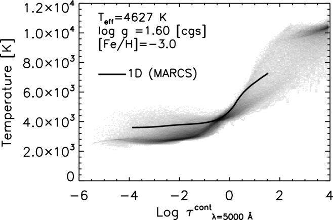
Figure 1: Gray shaded area: Temperature distribution as a function of continuum optical depth at $\lambda=5000$ Å in the 3D metal-poor red giant surface convection simulation used in the present analysis of HD122563; darker areas indicate values with higher probability. Solid line: Temperature stratification in the 1D marcs model atmosphere constructed for the same stellar parameters.

We use the stagger-code (Nordlund & Galsgaard, 1995) to carry out a 3D, radiative, hydrodynamical, simulation of convection at the surface of a red giant with approximately the same stellar parameters as HD122563, that is with an effective temperature $T\rm_{eff}$${\approx}4600$ K, a surface gravity ${\log}{g}=1.6$ (cgs), and a scaled solar chemical composition (Grevesse & Sauval, 1998) with [X/H]$=-3~{}$ for all metals. The equations for the conservation of mass, momentum, and energy are solved together with the radiative transfer equation on a discrete mesh with $480{\times}480{\times}240$ numerical resolution for a representative volume of stellar surface deep enough to cover about eleven pressure scale heights and large enough to incorporate about ten granules (${\sim}3700{\times}3700{\times}1100$ Mm³).

We adopt open boundaries at the top and at the bottom of the simulation domain, and periodic boundary conditions at the sides. We use a realistic equation-of-state (Mihalas et al., 1988) and continuous and line opacities by Gustafsson et al. (1975) and Kurucz (1992, 1993). To compute the radiative heating rates entering the energy conservation equation, we group the opacities in four opacity bins (Nordlund, 1982) and solve the radiative transfer equation for each bin along the vertical and eight inclined rays. We assume local thermodynamic equilibrium (LTE) and treat scattering as true absorption.

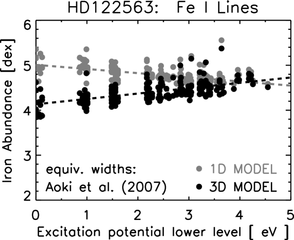
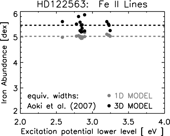
Figure 2: HD122563: Iron abundance derived from Fe i (left panel) and Fe ii lines (right panel) as a function of lower excitation potential; black (grey) filled symbols represent the results of the 3D (1D) analysis. The equivalent widths of the lines are taken from Aoki et al. (2007).

The predicted temperature and density stratification as well as the dynamics of the gas flows are qualitatively very similar to the ones reported for previous simulations of convection at the surface of red giants (Collet et al., 2007) and solar-type stars (Stein & Nordlund, 1998; Asplund & García Pérez, 2001). Warm, isentropic gas ascends from the bottom and, as it approaches the optical surface, it begins to cool by photon losses. Near the surface, the opacity behaves as a strongly sensitive function of temperature and decreases rapidly as the gas cools radiatively. As the gas becomes less opaque, photons escape more easily, lowering the temperature even further and cooling the gas to the point that it becomes negatively buoyant and starts to sink downward. This positive feedback causes a sudden drop of the gas temperature from ${\sim}10\,000$ K to ${\sim}5\,000$ K, which in the present metal-poor red giant simulation takes place within a distance of typically ${\sim}30$ Mm or less from the optical surface resulting in very steep vertical temperature gradients. The optical surface also appears to be very corrugated, with optical depth unity occurring over a large range of geometrical depths (${\sim}250$ Mm).

The temperature stratification as a function of optical depth for a typical simulation snapshot is shown in figure 1. Superimposed is the corresponding stratification from a 1D, LTE, plane-parallel, hydrostatic marcs model atmosphere (Gustafsson et al., 1975; Asplund et al., 1997) computed for the same stellar parameters. The temperatures in the upper photospheric layers of the 3D simulation are significantly lower (by ${\sim}1000$ K, on average) than in 1D. This disparity can be explained considering that in stationary hydrostatic and in time-dependent hydrodynamical models the mechanisms controlling the energy balance in the upper photosphere are effectively different: radiative equilibrium, in 1D, and radiative heating and adiabatic cooling due to gas expansion, in 3D (see Asplund et al., 1999; Collet et al., 2007).

We use the red giant surface convection simulation as a 3D, time-dependent, hydrodynamical model atmosphere to compute spectral lines for neutral and singly ionized Fe as well as for a number of molecules (e.g., OH, CH, and CN), under the assumption of LTE. We derive Fe and O abundances by reproducing the measured equivalent widths of Fe i and Fe ii (Aoki et al., 2007) and infrared (IR) vibrational-rotational OH lines at $1.6$ $\mu$m (Barbuy et al., 2003). We then compare the resulting abundances with the ones derived with the corresponding 1D marcs model atmosphere, assuming LTE and adopting a micro-turbulence of $2.0$ $\mathrm{kms}^{-1}$ for the 1D spectral line formation calculations.

3 Results and Discussion

Figure 2 shows the Fe abundance derived from Fe i and Fe ii spectral lines as a function of lower excitation potential. The systematic cooler upper photospheric temperature stratification of the 3D model atmosphere compared with the 1D model result in significant differences between the 3D and 1D LTE ionization equilibria. In particular, the fraction of neutral Fe in those layers is, on average, higher in the 3D model than in 1D. Hence, at a given abundance, synthetic Fe i lines tend to be stronger in 3D than in 1D, and a lower abundance is therefore required in 3D to match the observed equivalent widths of Fe i lines. Conversely, the Fe abundance derived from Fe ii lines is larger in the 3D case than in the 1D one. As a consequence, the difference between the Fe abundance values determined from Fe i and Fe ii lines actually increases when going from 1D to 3D. We also observe trends in the Fe abundance derived from Fe i lines with excitation potential in both 1D and 3D, but with opposite slopes in the two cases. Such trends as well as the difference between the Fe abundance determinations from neutral and singly ionized iron lines are possibly due to the neglected departures from LTE in the line formation calculations and/or to shortcomings still present in the model atmospheres.

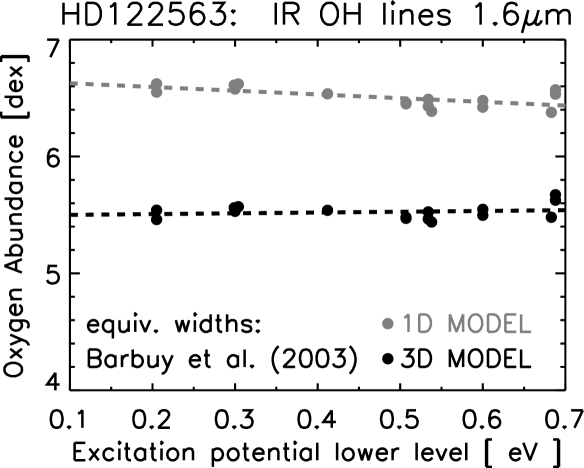
Figure 3: HD122563: Oxygen abundance derived from IR OH lines at $1.6$ $\mu$m as a function of lower excitation potential; black (grey) filled symbols indicate the results of the 3D (1D) analysis. The equivalent widths of the lines are taken from Barbuy et al. (2003).

Due to the highly non-linear temperature sensitivity of molecule formation, the differences between the 3D and 1D temperature stratifications also lead to radically different molecular equilibria in the two kinds of models. From the analysis of CH lines at $4300$ Å, the derived 3D carbon abundance is ${\sim}0.2$ dex lower than the 1D value. The 3D$-$1D nitrogen abundance difference estimated from the analysis of CN lines at $3880$ Å is even more pronounced and reaches ${\sim}1$ dex. Figure 3 shows the 3D and 1D oxygen abundances determined from the IR OH lines: again, the 3D abundance is lower by ${\sim}1$ dex than the 1D one. The 3D oxygen abundance values show no trend with lower excitation potential, which is reassuring as it suggests that the temperature gradient in the OH line formation region is probably well reproduced by the 3D simulation. The 1D oxygen abundance values show instead a decreasing, although relatively shallow, trend with excitation potential.

We also determine the 3D and 1D oxygen abundance from the forbidden [O i] line at $6300$ Å: we find that the 3D$-$1D abundance difference amounts to only $-0.15$ dex for this line. When we apply such 3D$-$1D abundance corrections to the oxygen abundances derived by Barbuy et al. (2003) we find the corrected values from [O i] and OH lines to be discrepant. The reasons for this discrepancy need be investigated further. It may indicate that the temperature stratification predicted by the present simulations is still not accurate enough. We are currently re-running the metal-poor red giant simulation with an improved and more accurate binning scheme by Trampedach et al. (2009): preliminary tests show that the resulting vertical temperature gradient in the atmosphere tends to become shallower and the differences with the 1D upper photospheric stratification appear smaller. We need however to wait for the simulation to fully relax before drawing conclusions about the consequences for spectral line formation and abundance analysis. Also, one would need to investigate other sources of possible systematic errors such as the treatment of scattering as true absorption in the convection simulations, and, more importantly, the possibility of departures from LTE in the calculation of excitation, ionization and molecular equilibria.

References

- Aoki et al. (2007) Aoki, W., Honda, S., Beers, T. C., et al. 2007, ApJ, 660, 747
- Asplund & García Pérez (2001) Asplund, M. & García Pérez, A. E. 2001, A&A, 372, 601
- Asplund et al. (1997) Asplund, M., Gustafsson, B., Kiselman, D., & Eriksson, K. 1997, A&A, 318, 521
- Asplund et al. (1999) Asplund, M., Nordlund, Å., Trampedach, R., & Stein, R. F. 1999, A&A, 346, L17
- Barbuy et al. (2003) Barbuy, B., Meléndez, J., Spite, M., et al. 2003, ApJ, 588, 1072
- Collet et al. (2007) Collet, R., Asplund, M., & Trampedach, R. 2007, A&A, 469, 687
- Cowan et al. (2005) Cowan, J. J., Sneden, C., Beers, T. C., et al. 2005, ApJ, 627, 238
- Grevesse & Sauval (1998) Grevesse, N. & Sauval, A. J. 1998, Space Sci. Rev., 85, 161
- Gustafsson et al. (1975) Gustafsson, B., Bell, R. A., Eriksson, K., & Nordlund, Å. 1975, A&A, 42, 407
- Kurucz (1992) Kurucz, R. L. 1992, Revista Mexicana de Astronomia y Astrofisica, 23, 181
- Kurucz (1993) Kurucz, R. L. 1993, Kurucz CD-ROMs, Vol. 2–12, Opacities for Stellar Atmospheres (Cambridge, Mass.: SAO)
- Mihalas et al. (1988) Mihalas, D., Däppen, W., & Hummer, D. G. 1988, ApJ, 331, 815
- Nordlund (1982) Nordlund, Å. 1982, A&A, 107, 1
- Nordlund & Galsgaard (1995) Nordlund, Å. & Galsgaard, K. 1995, A 3D MHD code for Parallel Computers
- Stein & Nordlund (1998) Stein, R. F. & Nordlund, Å. 1998, ApJ, 499, 914
- Trampedach et al. (2009) Trampedach, R. et al. 2009, in prep.