In-Network Outlier Detection in Wireless Sensor Networks

Abstract

To address the problem of unsupervised outlier detection in wireless sensor networks, we develop an approach that (1) is flexible with respect to the outlier definition, (2) computes the result in-network to reduce both bandwidth and energy usage, (3) only uses single hop communication thus permitting very simple node failure detection and message reliability assurance mechanisms (e.g., carrier-sense), and (4) seamlessly accommodates dynamic updates to data. We examine performance using simulation with real sensor data streams. Our results demonstrate that our approach is accurate and imposes a reasonable communication load and level of power consumption.

1 Introduction

Outlier detection, an essential step preceding most any data analysis routine, is used either to suppress or amplify outliers. The first usage (also known as data cleansing) improves robustness of data analysis. The second usage helps in searching for rare patterns in such domains as fraud analysis, intrusion detection, and web purchase analysis (among others).

Several factors make wireless sensor networks (WSNs) especially prone to outliers. First, they collect their data from the real world using imperfect sensing devices. Second, they are battery powered and thus their performance tends to deteriorate as power dwindles. Third, since these networks may include a large number of sensors, the chance of error accumulates. Finally, in their usage for security and military purposes, sensors are especially prone to manipulation by adversaries. Hence, it is clear that outlier detection should be an inseparable part of any data processing routine that takes place in WSNs.

Simply put, outliers are events with extremely small probabilities of occurrence. Since the actual generating distribution of the data is usually unknown, direct computation of probabilities is difficult. Hence, outlier detection methods are, by and large, heuristics. Because the problem is fundamental, a huge variety of outlier detection methods have been developed. In this paper we focus on non-parametric, unsupervised methods. A simplistic implementation of these methods would require centralization of the data. Such centralization is hard and costly in WSNs as it demands high bandwidth and requires reliable message transmission over multiple hops, which is both costly and difficult to implement.

We developed a technique for the computation of outliers in WSNs. This technique (1) is flexible with respect to the outlier definition, (2) computes the result in-network to reduce both bandwidth and energy usage GuptaKumar , (3) only uses single hop communication thus permitting very simple node failure detection and message reliability assurance mechanisms (e.g., carrier-sense), and (4) seamlessly accommodate dynamic updates to data. In addition to these essential features, the algorithm presented here also has two highly desirable properties: it is generic – suitable for many outliers detection heuristics and its communication load is proportional to the outcome (i.e. the number of outliers reported).

We exemplify the benefits of our algorithm by implementing it using two different outlier detection heuristics and simulating 53 sensors using the SENSE sensor network simulator sense:2004 with real sensor data streams. Our results show that the algorithm converges to an accurate result with reasonable communication load and power consumption. In most tested cases, our algorithm’s performance bests that of a centralized approach.

2 Motivating Application

The potential importance of efficient outlier detection in wireless sensor networks is best understood in the context of popular applications of those systems. Consider, for instance, the acoustic source localization problem. In this problem, a set of synchronized sensors all register the arrival of a specific sound at a certain time. Given the distance of two sensors from one another and the time difference of arrival (TDOA) of the sound, the potential locations of the source vis-a-vis the two sensors can be deduced. Given data from several sensors, the possible relative locations (each a hyperbola in the plane) can be intersected, and the location of the source can be pinpointed (see, for example Ajdler04sourceLocalization ; CounterSniper and Fig. 1).

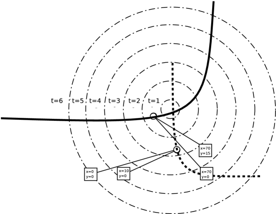
Figure 1: The expansion of a sound over time and the possible source location as computed by two different pairs of sensors according to the time difference of arrival. The origin of the sound lays in the intersection of the two hyperbola.

While the theoretic framework of TDOA based source location is simple and clear, the problem becomes much more complex in reality. Firstly, the real terrain in which the problem occurs is rarely flat, or an unobstructed three-dimensional space. Secondly, echos and multiple concurrent sounds may add many possible hyperbolas from which the relevant ones need be selected. Last, and perhaps most importantly, the method is sensitive to erroneous initializations in terms of sensor synchronization and positioning, as well as to the possible degradation of these factors when sensors’ power dwindles. All these factors amount to a multiplicity of possible hyperbolas, only few of which intersect at the correct location of the source.

In fact the similar principal of localization applies in a broader setting, in which imprecise detection by a single sensor, regardless of its modality (e.g., acoustic, seismic, visual, electromagentic, etc.) is applied in so called binary sensing object location WBS09 in which a group of neighboring nodes cooperate to narrow the object location. In fact, a detection, true of false, of object presence in a sensing range of sensor will trigger a tracking algorithm or even the entire tracking service CJ-SOA09 . Hence, to avoid the costs associated with unnecessary execution of the tracking algorithm or service, wrong data (whatever the cause) must be detected and removed. There are ample methods in which such detection and removal can be carried out (e.g. Maximum Likelihood ML-WSN ). However, they all rely on centralization of all of the data for processing. Such centralization would likely be unacceptably costly in wireless sensor networks for two main reasons. First, because a huge portion of the energy of a sensor would be spent on relaying data of other sensors. Second, because naive centralization would make no use of old data when new data arrives, even if the data changes only slightly. For instance, if a certain sensor produces unwanted signals (say, due to a local noise source), that sensor and every sensor relaying its data to the center would constantly waste energy on centralization of the data even though it might clearly be undesired.

It is therefore of high importance to be able to perform data cleansing in the network concurrent to any decision protocol. With the method suggested in this paper, sensors can constantly and efficiently prune away data which seems false. Only then, and only if the remaining data seems to require further analysis, would the more complex and costly procedure for source localization be executed. In this way, much energy can be saved and system lifetime can be extended.

This paper presents an efficient algorithm for in-network outlier detection. The algorithm is generic, permitting several definitions of an outlier. The experimentation and simulation results are presented for this aglorithm and not for the entire motivating example because source localization and tracking using wireless sensor networks is well understood (e.g., see beck2008exact ).

3 Related work

3.1 Outlier detection

Outlier detection is a long studied problem in data analysis, we provide only a brief sampling of the field. Hodge and Austin HA:2004 present a survey focusing on outlier detection methodologies based on machine learning and data mining. These include distance and density-based unsupervised methods, feed-forward neural networks and decision tree-based supervised methods, and auto-associative neural network and Hopfield network-based methods. Barnett and Lewis BL:1994 provide a survey of outlier detection methodologies in the statistics community.

Our algorithm is flexible in that it accommodates a whole class of unsupervised outlier detection techniques such as (1) distance to $k^{th}$ nearest neighbor RRS:2000 , BS:2003 , (2) average distance to the $k$ nearest neighbors AP:2002 , BS:2003 , and (3) the inverse of the number of neighbors within a distance $\alpha$ KN:1998 (see Section 4 for details).

3.2 Wireless sensor networks

WSNs combine the capability to sense, compute, and coordinate their activities with the ability to communicate results to the outside world. They are revolutionizing data collection in all kinds of environments. At the same time, the design and deployment of these networks creates unique research and engineering challenges due to their expected large size (up to thousands of sensor nodes), their often random and hazardous deployment, obstacles to their communication, their limited power supply, and their high failure rate.

The software for WSNs needs to be aware of their limitations and features. The most important among these are limited power, high communication cost, and limited direct communication range. In mobicom99 , Estrin et al. introduce scalable coordination as an important component of the needed software. A survey of the state-of-the-art in WSNs is given in in computer-networks02 . Another survey comm-magazine02 focuses on challenges arising from specific applications such as military, health care, ecology, and security.

Energy-efficiency, a cardinal WSN requirement, is often achieved by minimizing communication using topology-control algorithms that dictate the active/sleep cycles of sensor nodes. Examples include Geographic Adaptive Fidelity (GAF) mobicom01 , ASCENT ascent , STEM stem , and ESCORT icn05 . While the focus of this paper is on WSN outlier detection, the challenge is the same as in the above mentioned works. Hence, while we do not propose a topology-control algorithm, we aim to design an energy-efficient algorithm by minimizing the required communication overhead.

Other research efforts have also addressed the issue of developing a framework for distributed outlier detection in WSNs.

The framework of Zhuang et al. ZCWL:2007 use a weighted moving average approach to smooth noise from the data stream arriving at each sensor. In addition to temporal information (past data values), sensors also use data from neighboring sensors (spatial smoothing) to reduce the rate at which data values are propagated to the sink. When an observed data value remains within the established spatio-temporal trend, it is not propagated. Their approach differs from ours in that theirs does not seek to detect outliers.

The framework of Sheng et al. SLMJ:2007 allows the discovery of k-nearest-neighbor based outliers: points whose distance to their k-nn exceeds a fixed threshold or the top n points with respect to the distance to their k-nns. Each sensor maintain a histogram-type summary of pertinent information over a sliding window of its data points. This summary is propagate to a sink node. The sink node collects the summaries and queries the network for any additional information needed to correctly determine the outliers over the whole network. The use of summaries allows their approach to use less communication than a naive, centralized approach. Their approach differs from ours in several ways. First, they only detect outliers over one dimensional data. Indeed, extending their approach to more dimensions is complicated by the fact that compact, multi-dimensional histograms are difficult to build. Second, they only consider the two k-nn based outlier definitions described above. While our approach encompasses these and more. Thirdly, their approach only applies in settings where spatial proximity is unimportant (data from all sensors, near and far, is used in determining outliers). We have developed an approach that considers spatial proximity (”semi-local” outlier detection) as well as one that does not.

The framework of Subramaniam et al. SPPKG:2006 requires the sensors to maintain a tree communication topology and computes outliers based on an estimate of the underlying probability distribution from which the data arises. Such an estimate is computing by each sensor maintaining a random sample of its data observations. Our approach differs in at least four ways. First, ours does not make any assumptions about the communication topology (e.g. it is a tree), save that it is connected. Second, ours computes outliers with respect to all of the data observations at each sensor, not a sample. Third, ours can smoothly take into account spatial proximity among the sensors (“semi-local” outliers) while Subramaniam does not focus on this task. Fourth, our approach is designed to smoothly adjust to changes in the underlying network topology while Subramaniam’s requires that the underlying communication tree be reestablished by other means before their algorithm can resume operation.

The framework of Janakiram et al. JRK:2006 is based on a Bayesian Belief Network (BBN) that has been constructed over the WSN (and distributed to each sensor). Using this, each sensor can estimate the likelihood of an observed tuple and, therefore, detect outliers. However, Janakiram does not discuss the problem of updating the BBN given network/data change. It is not clear to what extent the BBN construction phase can by carried out in-network. Our approach differs in that it is in-network and designed to smoothly adjust to changes in data/network.

The framework of Zhuang and Chen ZC:2006 uses a wavelet based technique for correcting large isolated spikes from single sensor data streams. A dynamic time warping (DTW)distance-based technique is also used to identify more steady intervals of erroneous sensor data by comparing the data streams of spatially close sensors assumed to produce similar data streams. To reduce energy consumption, anomalous data streams are not transmitted to the base station. Our method is similar in that it is in-network. However, Zhuang and Chen’s use of DTW is tightly integrated with a minimum hop count routing algorithm, which makes the approach more restrictive than ours.

Rajasegarar et al. RLPB:2006 describe an approach that is based on distributed non-parametric anomaly detection and requires sensors to maintain a tree communication network topology. Here each sensor clusters its sampled measurements using a fixed-width clustering algorithm, then extracts statistics of the clusters (i.e., the centroid and number of contained data vectors) and then sends them its parent node. The parent uses its children’s’ cluster statistics to form a merged cluster and then transmits that cluster to its parent. This process continues recursively until the base station receives all clusters, after which it will perform anomaly detection to identify all outliers. While this approach supports energy-efficiency by distributing the clustering operation throughout the network, anomaly detection is only performed at the base station. Our approach differs in that it distributes the anomaly detection process itself throughout the network, quickly enabling nodes to identify outliers and autonomously make further data processing decisions. Also, our approach does not rely on the use and maintenance of a routing tree and hence, is able to smoothly adjusts to changes in the underlying network topology.

Adam et al. AJA:2004 address the issue of accounting for spatially neighboring peers when detecting outliers in sensor networks. However, they assume the sensor datasets are centralized and the outlier processing is carried out there. They do not consider the problem of carrying out the outlier detection in-network as we do.

Palpanas et al. PPKG:2003 propose a technique for distributed deviation detection using a network hierarchy of low and high capacity sensors that are differentiated with respect to processing power and communication range. Here, low capacity sensors aim to detect local outliers while high capacity sensors detect more spatially dispersed outliers using an aggregation of low capacity sensors’ data. Kernel density estimators are used to model the distribution of data values reported by sensors and distance-based detection techniques are used for identifying outliers. The authors present no formal evaluation of the proposed technique. Our approach differs in that it does not rely on a hierarchy of device capabilities.

The framework of Radivojac et al. RKSO:2003 addresses the process of sensors learning data distributions from class-imbalanced data. Here, sensors send data points to a central base station which is tasked with generating a classification model from class-imbalanced data (i.e., having an abundant number of negative samples and a small amount of positives). The model is generated using a neural network classifier, after which the base station distributes the model to the sensors for detection purposes. This process repeats throughout the lifetime of the network. A Bayesian classifier is also employed to extend the lifetime of the network by minimizing the total cost of detection and classification (e.g., costs of transmitting false-positives and false-negatives). Again, our framework differs in that it operates in-network as opposed to a centralized manner.

Our work in this paper is an extension of our preliminary work appearing in conference proceedings BSWGK:2006 . We have extended our preliminary work by providing complete correctness proofs for the global outlier detection algorithm. And, we have improved the experimental analysis of the global algorithm. We have also added the localized outlier detection algorithm and experimental analysis of it.

3.3 Distributed data mining

Distributed Data Mining (DDM) has recently emerged as an important area of research. DDM is concerned with analysis of data in distributed environments, while paying careful attention to issues related to computation, communication, storage, and human-computer interaction. Detailed surveys of Distributed Data Mining algorithms and techniques have been presented in Kargupta_97 , Kargupta_99 , Kargupta_04 . Some of the common data-analysis tasks include association rule mining, clustering, classification, kernel density estimation and so on.

Recently, researchers have started to consider data analysis and data mining in large-scale dynamic networks with the goal of developing techniques that are highly asynchronous, scalable, and robust to network changes. Efficient data analysis algorithms often rely on efficient primitives, so researchers have developed several different approaches to computing basic operations (e.g. average, sum, max, or random sampling) on dynamic networks. Mehyar et al. MSPLM:2007 develop an asynchronous, deterministic technique for computing an average over a large, dynamic network. Kempe et al. kempe03gossip and Boyd et al. BGPS:2005 investigate gossip based randomized algorithms. Jelasity and Eiben KJE:2003 develop the “newscast model”. Bawa et al. BGMM:2007 have developed an approach in which similar primitives are evaluated to within an error margin. Wolff et al. Majority-Rule-SMC-B develop a local algorithm for majority voting. Datta and Kargupta DK:2007 develop a technique for uniformly sampling data distributed over a large-scale peer-to-peer network. Wolff et al. WBK:2009 , Sharfman et al. SSK:2007 , and Bhaduri et al. BK:2008 develop techniques for threshold monitoring over a large, distributed set of data streams. Finally, some work has gone into more complex data mining tasks: association rule mining Majority-Rule-SMC-B , facility location KSW:2007 , decision tree induction BWGK:2008 , classification through meta-learning LXLS:2007 (all four based on local majority voting), genetic algorithms CDS:2003 , k-means clustering DGK:2006 WKK:2006 , web user community formation DBLK:2008 , hidden variable distribution estimation in a wireless sensor network MK:2008 , outlier detection in distributed data streams OGP:2006 SHYZJ:2007 . The last two papers address a related problem as we do: outlier detection over multiple distributed data streams. However, their work is not designed for a WSN. For example, they rely on frequent whole-network broadcasts (Otey) or information centralization at a leader node (Su) – arguably reasonable approaches in a wired network, but very costly in a WSN. Finally, an overview of the problem of carrying out data mining on data distributed over a dynamic peer-to-peer network is given in DBGWK:2006 .

4 Preliminaries

4.1 Outlier Detection Defined

Let $\mathbb{D}$ be a data space. We adopt a commonly used approach in the data mining/machine learning literature such that outliers are defined by specifying ranking function, $R$. This function maps $x\in\mathbb{D}$ and finite $D\subseteq\mathbb{D}$ to a non-negative real number $R(x,D)$ indicating the degree to which $x$ can be regarded as an outlier with respect to a dataset $D$. Some common examples of $R$ include (among others): the distance to the $k^{th}$ nearest neighbor (RRS:2000 , BS:2003 ); the average distance to the $k$ nearest neighbors (AP:2002 , BS:2003 ); and LOF (breunig00lof ). We assume that a fixed total linear order, $\prec$, on $\mathbb{D}$ is used as a tie-breaking mechanism to ensure that $R(.,Q)$ creates a total linear ordering on $\mathbb{D}$ for any finite $Q\subseteq\mathbb{D}$. This is equivalent, for our purposes, to assuming, without loss of generality, that $R(.,Q)$ is one-to-one.

$R$ is assumed to satisfy the following two axioms. Given $x\in\mathbb{D}$, for all finite $Q_{1}\subseteq Q_{2}\subseteq\mathbb{D}$: anti-monotonicty, $R(x,Q_{1})\geq R(x,Q_{2})$; smoothness, if $R(x,Q_{1})>R(x,Q_{2})$, then there exists $z\in Q_{2}\setminus Q_{1}$, such that $R(x,Q_{1})>R(x,Q_{1}\cup\{z\})$. The anti-monotonicty axiom is similar to the Apriori rule in frequent itemset mining AMS:1996 . The smoothness axiom, intuitively, states that $R$ changes gradually. As more points are added to $Q_{1}$, the rating function changes gradually to $R(x,Q_{2})$. Of the examples in the previous paragraph, all but LOF satisfies these assumptions, assuming, as we do, the use of a tie-breaking mechanism as described in the previous paragraph.

Given $n$ a user-defined parameter and a finite dataset $D\subseteq\mathbb{D}$, the outliers of $D$ are denoted $O_{n}(D)$ and are defined to be the top $n$ points in $D$ with respect to $R(.,D)$ (if $|D|<n$, then $O_{n}(D)$ is defined to be $D$).

4.2 Distributed System Set-up

The distributed system architecture we assume consists of a collection of sensors, $p_{i}$, each holding a finite dataset $D_{i}\subseteq\mathbb{D}$. Sensors communicate by exchanging messages to their immediate neighbors as defined by an undirected graph. We assume that messages are reliable, i.e. a message sender can assume that if a message is not recieved, then the sender will be informed); and each sensor $p_{i}$ can accurately maintain the list of its immediate neighbors, $\Gamma_{i}$, in the graph. Our algorithms work as long as there exists a path, possibly unknown, from each sensor to every other sensor. Note that, message reliability is difficult to fully maintain in a WSN – some message dropping is expected. While our algorithm assumes no message dropping, modest violation of this assumption in our experiments did not effect accuracy significantly.

5 Global Distributed Outlier Detection Algorithm

In this section, we describe a distributed algorithm by which sensors, each assumed to know $R$ and $n$, compute $O_{n}(D)$ where $D$ $=$ $\bigcup_{i}D_{i}$ (global outlier detection). In a wireless sensor network, it can be desirable for sensors to find outliers only with respect to the data contained in nearby sensors, rather than the entire network (semi-global outlier detection). In the next section 6, we describe how to modify the global outlier detection algorithm to act in a semi-global manner.

At any point in time, $p_{i}$ keeps track of the data points it has sent to or received from its neighbor $p_{j}$ at some past time. Let $D^{i}_{i,j}$ denote the set of points sent from $p_{i}$ to $p_{j}$, and, $D^{i}_{j,i}$ deonte the set of points sent from $p_{j}$ to $p_{i}$. Importantly, $(D^{i}_{i,j}$ $\cup$ $D^{i}_{j,i})$ denotes the data points that $p_{i}$ can be sure are commonly held with $p_{j}$ (there may be more). Let $P_{i}$ denote $D_{i}\bigcup_{j\in\Gamma_{i}}D^{i}_{j,i}$, the set of points $p_{i}$ is holding at the current time. $p_{i}$ uses $P_{i}$ to compute an estimate of the overall correct answer, $O_{n}(D)$. This estiamte, henceforth called $p_{i}^{\prime}s$ estimate, is $O_{n}(P_{i})$, the set of outliers based on all the information availible to $p_{i}$ at the current time.

The algorithm does not assume any special sensors. Each sensor, $p_{i}$, asynchronously waits for an event to occur: (i) the algorithm is initialized, (ii) $D_{i}$ changes, (iii) a message is received from a neighbor, or (iv) a link goes up/down causing $p_{i}^{\prime}s$ immediate neighborhood to change (however, algorithm correctness requires that we assume the network remain connected). Note that, events for $p_{i}$ are entirely local and can be detected without the aid of any other sensors beyond the immediate neighborhood. Once $p_{i}$ detects an event, it will decide which of the points it is currently holding ($P_{i}$), if sent, could cause its neighbor, $p_{j}$, to change its estimate. $p_{i}$ then sends these points and adds them to $D^{i}_{i,j}$ ($p_{i}$ carries out this process separately for all of its neighbors).

Gradually, the points held by each sensor enlarges until enough overlap is obtained so that each sensor’s estimate is the correct answer, $O_{n}(D)$. This will be gauranteed to occur once each sensor, individually, decides that none of the points it is currently holding need be sent to its neighbors. At this point, the algorithm is terminated. To see how all of this works, consider an example.

5.1 Example

Let $R$ be the distance to the nearest neighbor and given $x\in\mathbb{D}$ and finite $P\subseteq\mathbb{D}$, $N(x,P)$ denotes the nearest neighbor of $x$ among points in $P$. Given finite $Q\subseteq\mathbb{D}$, $N(Q,P)$ denotes $\bigcup_{x\in Q}N(x,P)$. Let $n=1$ and consider a network of two sensors, $p_{i}$ and $p_{j}$, each initially holding the following one-dimentional datasets. The correct answer the algorithm will compute is $O_{n}(D)$ $=$ $\{0.5\}$.

• $D_{i}=\{0.5,3,6,10,11,\ldots,a\}$.

• $D_{j}=\{4,5,7,8,9,a+1,a+2,\ldots,a+b\}$.

• $D=D_{i}\cup D_{j}=\{0.5,3,4,5,6,7,8,9,10,11,\ldots,a,a+1,\ldots,a+b\}.$

Initially, $P_{i}=D_{i}$, $P_{j}=D_{j}$, and $D^{i}_{i,j}$ $=$ $D^{i}_{j,i}$ $=$ $D^{j}_{i,j}$ $=$ $D^{j}_{j,i}$ $=$ $\emptyset$. For simplicity, we will describe the algorithm in synchronous fashion starting with $p_{i}$. But, the ideas extend nicely to asynchronous operation.

1. $p_{i}$ computes its estimate as $O_{n}(P_{i})=\{6\}$ and then must compute the set of its data points that might cause $p_{j}$ to change its estimate if sent. We call these the sufficient points from $P_{i}$ for sensor $p_{j}$. Formally, we define a set $Z_{j}\subseteq P_{i}$ to be sufficient for $p_{j}$ if

   $$\left[O_{n}(P_{i})\cup N(O_{n}(P_{i}),P_{i})\right]\cup\left[N(O_{n}(D^{i}_{i,j}\cup D^{i}_{j,i}\cup Z_{j}),P_{i})\right]\subseteq Z_{j}.$$ (1)

   The rationale for the first part is simple. $O_{n}(P_{i})$ is necessary for $p_{j}$, because if $p_{i}$ is right in its estimate, then $p_{j}$ ought to know about it. Moreover, $p_{i}$ must also send $N(O_{n}(P_{i}),P_{i})$, because this allows $p_{j}$ to determine if any of its points can cause the ranking of the points in $O_{n}(P_{i})$ to change.

   The rationale for the second part is somewhat more complicated. In brief, if $p_{i}$ were to send $Z\subseteq P_{i}$ to $p_{j}$, then $p_{i}$ would also need to send $N(O_{n}(D^{i}_{i,j}\cup D^{i}_{j,i}\cup Z),P_{i})$. To avoid resending, $p_{i}$ requires that $N(O_{n}(D^{i}_{i,j}\cup D^{i}_{j,i}\cup Z),P_{i})$ is contained in $Z$. To understand the reasoning for all of this, consider that $(D^{i}_{i,j}\cup D^{i}_{j,i}\cup Z)$ is the total set of points $p_{i}$ knows $p_{j}$ has if $Z$ were to send $p_{j}$. Thus, $O_{n}(D^{i}_{i,j}\cup D^{i}_{j,i}\cup Z)$ is $p_{i}^{\prime}s$ best approximation to $p_{j}^{\prime}s$ estimate if $Z$ were to send $p_{j}$. Hence, $p_{i}$ computes its nearest neighbors to these, because, if $p_{i}$ is right in its approximation, it must ensure that $p_{j}$ have these neighbors since they could cause $p_{j}$ to change its estimate.

   Getting back to our example, observe that $O_{n}(P_{i})$ $\cup$ $N(O_{n}(P_{i}),P_{i})$ $=$ $\{3,6\}$. Moreover, $N(O_{n}(D^{i}_{i,j}\cup D^{i}_{j,i}\cup\{3,6\}),P_{i})$ $=$ $N(O_{n}(\{3,6\}),P_{i})$ $=$ $\{3\}$ $\subseteq$ $\{3,6\}$. Hence, $Z_{j}$ $=$ $\{3,6\}$ as this satisfies (1) above. So, $p_{i}$ sends $\{3,6\}\setminus(D^{i}_{i,j}\cup D^{i}_{j,i})$ $=$ $\{3,6\}$ and updates $D^{i}_{i,j}$ to $\{3,6\}$.

2. $p_{j}$ will receive these points and updates $D^{j}_{i,j}$ to $\{3,6\}$ (currently $D^{j}_{j,i}=\emptyset$). So, implicitly, $P_{j}$ now denotes $D_{j}\cup D^{j}_{i,j}$ $=$ $\{3,4,5,6,7,8,9,a+1,a+2,\ldots,a+b\}$. $p_{j}$ computes $O_{n}(P_{j})$ $\cup$ $N(O_{n}(P_{j}),P_{j})$ $=$ $\{3,4\}$ (assuming appropriate tie-breaking). Moreover, it can be seen that this satisfies (1). So, $p_{j}$ sends $\{3,4\}$ $\setminus$ $(D^{j}_{i,j}\cup D^{j}_{j,i})$ $=$ $\{3,4\}$ $\setminus$ $\{3,6\}$ $=$ $\{4\}$ and updates $D^{j}_{j,i}$ to $\{4\}$.

3. $p_{i}$ will receive these points and updates $D^{i}_{j,i}$ to $\{4\}$ (currently $D^{i}_{i,j}=\{3,6\}$). So, implicitly, $P_{i}$ now denotes $D_{i}\cup D^{i}_{j,i}$ $=$ $\{0.5,3,4,6,10,11,\ldots,a\}$. $p_{i}$ computes $O_{n}(P_{i})$ $\cup$ $N(O_{n}(P_{i}),P_{i})$ $=$ $\{0.5,3\}$. Moreover, it can be seen that this satisfies (1). So, $p_{i}$ sends $\{0.5,3\}$ $\setminus$ $(D^{i}_{i,j}\cup D^{i}_{j,i})$ $=$ $\{0.5,3\}$ $\setminus$ $\{3,4,6\}$ $=$ $\{0.5\}$ and updates $D^{i}_{i,j}$ to $\{0.5,3,6\}$.

4. $p_{j}$ will receive these points and updates $D^{j}_{i,j}$ to $\{0.5,3,6\}$ (currently $D^{j}_{j,i}=\{4\}$). So, implicitly, $P_{j}$ now denotes $D_{j}\cup D^{j}_{j,i}$ $=$ $\{0.5,3,4,5,6,7,8,9,a+1,a+2,\ldots,a+b\}$. $p_{j}$ computes $O_{n}(P_{j})$ $\cup$ $N(O_{n}(P_{j}),P_{j})$ $=$ $\{0.5,3\}$. Moreover, it can be seen that this satisfies (1). So, $p_{j}$ sends $\{0.5,3\}$ $\setminus$ $(D^{j}_{i,j}\cup D^{j}_{j,i})$ $=$ $\{0.5,3\}$ $\setminus$ $\{0.5,3,4,6\}$ $=$ $\emptyset$. i.e. nothing is sent.

   At this point the algorithm has terminated, both sensors are waiting for an event to occur and there are no messages in flight. $P_{i}$ and $P_{j}$ denote $\{0.5,3,4,6,10,11,\ldots,a\}$ and $\{0.5,3,4,5,6,7,8,9,a+1,a+2,\ldots,a+b\}$, respectively. Therefore $O_{n}(P_{i})$ $=$ $\{0.5\}$ $=$ $O_{n}(P_{j})$, which in turn, equals the correct answer $O_{n}(D)$. Observe that the total amount of communication (data points sent) was 4. The naive approach which centralized all the data on either $p_{i}$ or $p_{j}$ requires $\min\{a-6,b+5\}$ communication. For large $\min\{a,b\}$, the distributed algorithm requires much less communication.

5.2 The Algorithm

To translate the previous example into a formal algorithm for general $R$ (satisfying the anti-monotonicity and smoothness axioms), we must provide some definitions generalizing the role of $N(.,.)$. Given $x\in\mathbb{D}$ and finite $P\subseteq\mathbb{D}$, $Q_{1}\subseteq P$ is called a support set of $x\in\mathbb{D}$ over $P$ if $R(x,P)=R(x,Q_{1})$. Intuitively, all other points from $P$ can be discarded without affecting the rank of $x$. Using cardnality and the tie-breaking mechanism discussed earlier ($\prec$ a total linear order on $\mathbb{D}$), we can define a unique, smallest support set of $x$ with respect to $P$, denoted $[P|x]$. Given $Q\subseteq P$, let $[P|Q]$ denote $\bigcup_{x\in Q}[P|x]$. In the previous example, $R$ was the distance to the nearest neighbor, so, $[P|x]$ equaled $N(x,P)$ using $\prec$ to break ties.

With these more general definitions, we define a set $Z_{j}\subseteq P_{i}$ to be sufficient for $p_{j}$ if

$$\left(O_{n}(P_{i})\cup[P_{i}|O_{n}(P_{i})]\right)\cup\left([P_{i}|O_{n}(D^{i}_{i,j}\cup D^{i}_{j,i}\cup Z_{j})]\right)\subseteq Z_{j}.$$ (2)

Due to the broadcast nature of wireless sensor network communication, $p_{i}$ cannot send points to an single immediate neighbor without the other neighbors receiving them as well. In light of this, the algorithm accumulates all points (tagged with receipiant IDs) to be sent to all immediate neighbors in a single packet, $M$. When an immediate neighbor, $p_{j}$, receives $M$, the neighbor extracts those points that are tagged with ID $j$. If no points are tagged as such, $p_{j}$ does not regard receipt of $M$ as an event.

$p_{i}$ detects an event if one of the following occurs: (i) the algorithm is initialized, (ii) $D_{i}$ changes, (iii) $M$ is received and contains points tagged with $i$ (i.e. points are received from a neighbor), or (iv) a link goes up/down causing $p_{i}^{\prime}s$ immediate neighborhood to change however, algorithm correctness requires that we assume the network remain connected). In response, $p_{i}$ carries out the following algorithm whose pseudo-code is given in Global Outliers Detection Algorithm figure. First, $P_{i}$ is updated accounting for all $p_{j}$ from which points were recived in $M$. Only points not already in $P_{i}$ are added to $D^{i}_{j,i}$. The first two steps in the main for-loop (“For each $j\in\Gamma_{i}$, do”) compute a $Z_{j}$ satisfying (2), although the result is not guaranteed to be the smallest set to do so. The “If….then” in the main for-loop tests whether there are any points found sufficient for $p_{j}$ that $p_{i}$ cannot already be sure $p_{j}$ has, i.e. points in $Z_{j}$ but not in $D^{i}_{j,i}\cup D^{i}_{i,j}$. If any such points are found they are added to $M$ along with their recipiant ID $j$.

Algorithm 1

•   

    – Set $M=\emptyset$, and, update $P_{i}$ accounting for all neighbors $p_{j}$ from which points were recieved. For each point $x$ recieved from $p_{j}$, do the following. If $x$ is not already $P_{i}$, then add $x$ to $D^{i}_{i,j}$.

    – For each $j\in\Gamma_{i}$, do

    – – Set $Z_{j}$ $=$ $O_{n}(P_{i})\cup[P_{i}|O_{n}(P_{i})]$.

    – – Repeat until no change: $Z_{j}=Z_{j}\cup[P_{i}|O_{n}(D^{i}_{i,j}\cup D^{i}_{j,i}\cup Z_{j})].$

    – – If $Z_{j}\setminus(D^{i}_{i,j}\cup D^{i}_{j,i})$ is non-empty, then

    – – – Append $\langle j,Z_{j}\setminus(D^{i}_{i,j}\cup D^{i}_{j,i})\rangle$ to $M$.

    – – – Add points in $Z_{j}\setminus(D^{i}_{i,j}\cup D^{i}_{j,i})$ to $D^{i}_{i,j}$.

    – – End If.

    – End For.

    – If $M$ is non-empty, broadcast it to all sensors in $\Gamma_{i}$.

end

Figure 2: Global Outlier Detection

5.3 Streaming Data and Peer Addition/Deletion

In our experiments we assume a sliding window model (based on time) in processing the data stream arriving at each sensor. To do so, we assume each point is time-stamped when sampled by the sensor. Under the assumption that the sensor clocks are synchronized sufficiently well, sensor $p_{i}$ deletes all points in $P_{i}$ (regardless of where they were originally sampled) once thier time-stamp indicates they are no longer in the window.

The algorithm can be easily modified to accomidate the addition of sensors during operation. All that is required to do so is treat the arrival of a new sensor as an event for the new sensor and for all its immediate neighbors. The algorithm can also be modified to accomidate the removal of sensors (e.g. when their battery is depleted) assuming that the network remains connected. In the sliding window model, a simple strategy is to merely allow points that originated with the removed sensor to age out of the window at the expense of tolerating, strictly speaking, an inaccurate result until this happens. A more general and complex solution is to propogate messages into the network causing sensors to explicitly delete those points that originated with the removed sensor. We leave the details of this approach to future work.

5.4 Algorithm Correctness

The correctness of the algorithm can be proved in the following sense: if the data and network links remain static (and the network is connected), then communication will eventually stop at which point all sensors’ outlier estimate will equal $O_{n}(D)$. It is important to emphasize that this does not mean the algorithm cannot handle dynamic data or network links. Merely that, upon such a change, the algorithm will respond and converge on the correct answer. But, naturally, such convergence is gauranteed only if the data and network remain static long enough.

It is easy to see that, barring data or network change, the algorithm will always terminate. So, the proof proceeds in two steps. First, upon termination, all sensors have the same outlier estiamtes and support (Theorem 1). Second, the consistent outlier estimates shared by all sensors is indeed the correct one (Theorem 2). Proofs of Theorems 1 and 2 are provided in Appendix 9.

Theorem 1

Assuming a connected network, if for all sensors $p_{i}$: $D_{i}$ and $\Gamma_{i}$ do not change, then upon termination of the algorithm all sensors’ outlier estimates and supports agree: for all $p_{i},p_{j}$: $O_{n}(P_{i})=O_{n}(P_{j})$ and $[P_{i}|O_{n}(P_{i})]=[P_{j}|O_{n}(P_{j})]$.

Theorem 2

Assuming a connected network, if for all sensors $p_{i}$: $D_{i}$ and $\Gamma_{i}$ do not change, then upon termination of the algorithm, all sensors’ outlier estimate will be correct: for all $p_{i}$: $O_{n}(P_{i})=O_{n}(D)$.

Comments: 1) Theorem 1 holds without the smoothness axiom, hence, for any anti-monotonic $R$, upon convergence, all sensors will agree on their outlier estimate and support. However, without the smoothness axiom, Theorem 2 does not hold, i.e. the consistent outlier estimates might not be the correct one. There are counter-examples which show how an anti-monotonic, but not smooth $R$ cause the algorithm to terminate without all sensors agreeing upon the correct set of outliers.

2) For an arbitrary $R$, it is not clear how to efficiently compute $[P|x]$ and we do not address the issue. However, efficient computation is straight-forward for the $R$ we consider in our experiments: average distance to the $k^{th}$ nearest neighbor.

6 Semi-Global Distributed Outlier Detection Algorithm

It can be desirable for sensors to find outliers only with respect to the data contained in nearby sensors, rather than the entire network. In this section, we describe how to modify the global outlier detection algorithm to act in a semi-global manner. Under this approach, each sensor computes outliers only from within those points sampled in its spatial proximity.

To account for spatial locality, we use hop distance: the number of hops bewteen two sensors along their shortest path in the underlying communication network. Given integer $d$ and sensor $p_{i}$, let $D_{i}^{\leq d}$ denote the union of all $D_{j}$ such that $p_{j}$ and $p_{i}$ have hop distance no greater than $d$. The semi-global outlier detection problem requires each $p_{i}$ to compute $O_{n}(D_{i}^{\leq d}$). Setting $d$ to infinity yields the global outlier detection problem discussed earlier.

To account for hop distance, each data point $x$ has an additional field $x.hop$ (at birth $x.hop$ is set to zero). Let $x.rest$ denote all the remaining fields – these are the ones used by the rating function $R$. Given a set of points $Q$, for $0\leq h\leq d$, let $Q^{\leq h}$ be the set of points $x\in Q$ with $x.hop\leq h$. Let $[Q]^{min}$ be the result of replacing all points that differ only in their hop field by the point with the smallest hop field. For example, consider $Q=\{w,v,x,y,z\}$ where $w.rest=v.rest$, $x.rest=y.rest=z.rest$, and $v.rest\neq x.rest$. If $w.hop<v.hop$ and $x.hop<y.hop,z.hop$, then $[Q]^{min}$ $=$ $\{w,x\}$.

6.1 Semi-Global Outlier Detection Algorithm

The basic idea is that each sensor $p_{i}$ will run the global outlier detection algorithm over only those points arising on sensors within $d$ hops. At first glance, the following simple modification of the global algorithm seems adequate. Before $p_{i}$ sends a copy of a point, $x$, to its neighbors, it first increments $x.hop$ and sends only if $x.hop\leq d$. Unfortunately, such a simple modification will not work. It does not take into account the fact that $x$ should not have any effect on the outlier determination process of sensors $p_{j}$ whose distance from $p_{i}$ is more than $d-x.hop$. Examples can be demonstrated wherein this omission causes an incorrect overall result.

To avoid this problem, $p_{i}$ must partition $P_{i}$ into $d$ parts: $P_{i}^{\leq h}$ for $0\leq h\leq d-1$. For each, in essence, the global outlier detection algorithm is applied. Upon detecting an event (defined as before), $p_{i}$ carries out the following algorithm whose pseudo-code is given in the Semi-Global Outlier Detection Algorithm figure.

First, $P_{i}$ is updated accounting for all $p_{j}$ from which points were recived in $M$. Because of the hop fields, the update step is somewhat more complicated than that of the Global Outlier Detection Algorithm. A point $x$ from $p_{j}$ is added to $D^{i}_{j,i}$ if there does not exist $y\in P_{i}$ with $x.rest=y.rest$ ($x$ does not already appear in $P_{i}$). Or, if there does exist $y\in P_{i}$ with $x.rest=y.rest$, but $x.hop<y.hop$, then $x$ replaces $y$ in $P_{i}$ (updating as needed $D_{i}$ and $D^{i}_{f,i}$ for each $f\in\Gamma_{i}$). Note, there cannot be more than one $y$ with the same rest fields as $x$ since all but the point with the smallest hop would have been removed earlier.

Next, for each neighbor $p_{j}$ and each $0\leq h\leq d-1$, a set $Z_{j}^{h}$ is computed which satisfies (2) with $Z_{j}$, $P_{i}$, $D^{i}_{i,j}$, and $D^{i}_{j,i}$ replaced by $Z_{j}^{h}$, $P_{i}^{\leq h}$, $D^{i,\leq h}_{i,j}$, and $D^{i,\leq h}_{j,i}$, respectively. This computation is done by the first steps inside the nested for loops. Then, the hop field for each point in $Z_{j}^{h}$ is incremented in preparation for sending to $p_{j}$.

Once all $0\leq h\leq d-1$ have been processed for $p_{j}$ (the inner for loop completes), $Z_{j}^{1}\cdots Z_{j}^{d-1}$ are unioned and redundancies are eliminated. For any pair of points $x,y$ in $\bigcup_{h=0}^{d-1}Z_{j}^{h}$, if $x.rest=y.rest$ and $x.hop<y.hop$, then $y$ is dropped (this action is signified by the ‘min’ superscript in the step immediately after the inner for loop). Then, all points $x$ are removed from $Z_{j}$ if there exists a point $y$ in $(D^{i}_{i,j}\cup D^{i}_{j,i})$ with the same rest fields but $y.hop\leq x.hop$. If the resulting $Z_{j}$ is non-empty, then these points are be added to $M$ (along with ID $j$) for broadcast to neighbors. And, $D^{i}_{i,j}$ is updated by adding the points in $Z_{j}$.

Algorithm 2

•   

    – Set $M=\emptyset$, and, update $P_{i}$ accounting for all neighbors $p_{j}$ from which points were recieved. For each point $x$ recieved from $p_{j}$, do the following. If there does not exist $y$ in $P_{i}$ with $x.rest$ $=$ $y.rest$, then add $x$ to $P_{i}$ (and update $D^{i}_{i,j}$), otherwise if $x.hop<y.hop$, then replace $y$ with $x$ in $P_{i}$ (updating as needed $D_{i}$ and $D^{i}_{f,i}$ for each $f\in\Gamma_{i}$).

    – For each $j\in\Gamma_{i}$, do

    – – For $h=0$ to $d-1$

    – – – Set $Z_{j}^{h}$ $=$ $O_{n}(P_{i}^{\leq h})\cup[P_{i}^{\leq h}|O_{n}(P_{i}^{\leq h})]$.

    – – – Repeat until no change: $Z_{j}^{h}=Z_{j}^{h}\cup[P_{i}^{\leq h}|O_{n}(D^{i,\leq h}_{i,j}\cup D^{i,\leq h}_{j,i}\cup Z_{j}^{h})].$

    – – – Increment the hop field for each point in $Z_{j}^{h}$.

    – – End For.

    – – Set $Z_{j}=\left[\bigcup_{h=0}^{d-1}Z_{j}^{h}\right]^{min}$.

    – – Remove points $x$ from $Z_{j}$ such that there exists $y\in(D^{i}_{i,j}\cup D^{i}_{j,i})$ with $x.rest=y.rest$ and $y.hop\leq x.hop$.

    – – If $Z_{j}$ is non-empty, then

    – – – Append $\langle j,Z_{j}\rangle$ to $M$.

    – – – Update $D^{i}_{i,j}$ by adding the points in $Z_{j}$.

    – – End If.

    – End For.

    – If $M$ is non-empty, broadcast it to all sensors in $\Gamma_{i}$.

end

Figure 3: Semi-Global Outlier Detection

7 Performance evaluation

7.1 Experimentation setup

We used the SENSE wireless sensor network simulator sense:2004 to evaluate the performance of the global and semi-global outlier detection algorithms. Specifically, we analyzed the following metrics: (1) the accuracy of the algorithms in detecting outliers; (2) the average amounts of total energy, transmission energy, and receive energy consumed per node per sampling period; and (3) the minimum and maximum amount of energy consumed in the network. We observed both the global and semi-global outlier detection algorithms to be highly accurate as nodes converged upon the correct results approximately 99% of the time. We attribute any detection error to dropped packets. Since average detection accuracy was consistent across all simulation parameters, we did not include any accuracy-related plots in this manuscript.

Various scenarios were used to analyze the performance of our algorithms. First, we compared our algorithms’ energy usage against that of a purely centralized outlier detection algorithm. Here, all nodes periodically sent their sliding window contents to a central node which detected outliers based on the unioned data sets and returned the outliers back to the nodes. For simplicity, we configured the centralized algorithm to calculate only global outliers since for this algorithm, energy usage is independent of whether global or semi-global outliers are detected. iAlso, all algorithms (including the centralized solution) were evaluated using the following two outlier ranking functions ($R$): distance to nearest neighbor (NN) and average distance to k nearest neighbors (KNN).

We chose to use a centralized algorithm for our comparison because, to the best of our knowledge, there exist no comparable distributed solutions for WSN outlier detection. We find such a comparison to still be valid as many WSN deployments continue to employ centralized configurations, citing ease of administration as well as maintenance of a single (and ”‘standard”’) point of interface with the growing number of applications and systems in the sense-and-respond computing domain. Such reasons, however, do not preclude the utility of a distributed algorithm such as ours, since it remains very useful as a general data processing solution for a wide range of applications, whether they are centralized are not.

For our data sets, we used real-world recorded sensor data streams from sensordata , in which distributed data samples are both spatially and temporally correlated. The data set we used was composed of series of data samples describing environmental phenomena such as heat, light, and temperature from 53 sensors which periodically transmitted individual data samples to a central base station. The data set did contain missing data points, which to the best of our knowledge was largely due to packet loss. Hence, we replaced missing data points with the average values of the data points within sliding windows preceding the missing points. This helped retain the temporal trends of the data streams. The data points we used contained the following features: (1) ID of the sensor that produced the data point; (2) epoch (sequential number denoting the data point’s position in the sensor’s entire stream); (3) data value (we specifically used temperature); and (4) x,y location coordinates. We used the data points’ temperature value and location coordinates as inputs into the outlier rating functions. The location coordinates can represent either the place of measurements or an estimate of a position of a target or some other spatial information. It is important to note that these coordinates are a part of the data on which our algorithm works in the example. They might suffer errors, and become anomalous, just as would any other attribute of the data, due to an inaccurate initialization, power degradation, or a transmission error. The algorithm itself, however, would work the same regardless if such coordinates are given or not.

We originally simulated two networks based on the coordinates of the sensors in the data set: the first of size 32 nodes (which included a uniformly random sampling of the full network) and the second of size 53. The purpose of simulating two networks was to examine how well the algorithm scaled with the size of the network. We found that the as the network size increased, the performance benefit of the distributed algorithms increased in comparison to the centralized algorithms and that performance trends for different test variables were generally the same. Hence, we did not include any detailed results associated with the smaller network in this manuscript.

We simulated a terrain of size 50m$\times$50m. Most hardware specifications claim that a sensor node’s transmission range typically reaches up to approximately 250m, when properly elevated. However, when placed on the ground the reported ranges are much smaller zuniga04 and for reliable communication indoor using Crossbow motes, the effective range drops to a few meters szymanski07 . Therefore, we configured all nodes to have a uniform transmission range of approximately 6.77m. We also used the hardware energy model based on the Crossbow mote specifications motespecs with a transmit/receive/idle power setting of 0.0159W/0.021W/3e-6W (assuming a 3V power source). We simulated the wireless transport medium using the free-space signal propagation model.

Two protocols were used for routing. For the distributed algorithms, we used simple broadcast (as opposed to unicast) transmission with promiscuous listening that allowed all nodes to send data points to all their adjacent neighbors using one transmission. For the centralized algorithm, we used the well accepted AODV perkins97ad wireless routing protocol for multi-hop communication. We note that a simple end-to-end acknowledgment mechanism was also used to reinforce reliable communication. While alternative protocols do exist for more data-centric and energy-efficient communication, our main goal was to compare the overhead between the algorithms in a straight-forward manner without having to involve ourselves with balancing various advantages towards either algorithm.

All simulations were run for 1000 seconds of simulated time and were repeated four times using different random number generator seed values to obtain averaged results. As shown in the following plots, we collected results for different values of the following algorithm parameters: (1) the length of the node’s sliding window, w; and (2) the number of outliers to be reported, n. Additionally, for the distributed localized outlier detection algorithm, we varied the hop diameter for the localized outlier detection algorithm for from one to three hops. The labeling of the data in the plots is as follows: (1) $Centralized$ for results obtained with the centralized algorithm; (2) $Global-NN$ and $Global-KNN$ for results obtained using distributed global outlier detection with NN and KNN outlier detection ranking functions ($R$), respectively; and (3) $Semi-global,epsilon=x$ for all results obtained using distributed localized outlier detection where $x$ is the value of the hop diameter of the spatial extent outlier detection. For brevity, we will often refer to the different algorithms by these labels.

7.2 Experimentation results

Figure 4: Average transmission and receive energy consumed per node per sample interval vs. $w$ ($n$=4, $k$=4) for global outlier detection.

7.2.1 Effect of sliding window size

The plots in Figure 4 compare the rate of energy usage of the network between using the centralized algorithm and the distributed algorithm for global outlier detection as $w$ increases and $n$ and $k$ remain fixed at 4. Here, we show separate plots for transmission (TX) and receive (RX) energy for the reader who is interested in the disparity between the energy consumption due to different radio operations. We note that data points are missing for Global-KNN at $w$=40, due to the inability of our computing resources to complete simulations for this particular algorithm at the given parameter value. However, preliminary results based on similar simulations and statistics are shown in BSWGK:2006 . Since the trends between both sets of results are nearly identical for the non-missing data points, it is reasonable to extrapolate the values of the missing points here.

Both figures show that as $w$ increases, Global-NN is the only algorithm that reduces its energy usage. Figure 4 shows that Global-NN eventually becomes the most energy-efficient solution given the domain of $w$. We attribute Global-NN’s reduction in energy usage to an increasing amount of incoming data redundancy as the size of the sliding window increases. Since Global-NN only uses one supporting point to determine an outlier, the probability of finding new outliers or supports with this scheme in each new time interval as the sliding window increases is low.

Regarding the energy consumption of Global-KNN and Centralized, Figure 4 reveals trends of increasing energy consumption as $w$ increases. However, given comparable results in BSWGK:2006 , we can extrapolate that Global-KNN’s amount of energy consumption is a concave increasing function of $w$, whereas Centralized’s is a convex increasing function, which makes the latter comparatively less energy-efficient in that it approaches a point of network failure at a higher rate. In comparison to Centralized, the energy trend for Global-KNN for this data set indicates that when global outliers are defined by multiple supporting points (in this case 4), the increasing size of the time interval from which the points are chosen has a less drastic effect on the number of messages required for the algorithm to converge. Overall, in cases where a user prefers to use more supporting points and a larger sliding window to define outliers, energy usage will be higher than using Global-KNN, but it is still more beneficial to use a distributed solution.

Figure 5: Average, minimum, and maximum amount of energy consumed by a node for global outlier detection.

Figure 5 shows the minimum, average, and maximum amounts of energy consumption for a sensor node as $w$ increases. Since we limit our focus primarily to the $range$ of a sensor’s energy consumption, with the intent of analyzing how energy is balanced under the different algorithms, we present data in terms of total energy consumption. The analysis of TX and RX energy have less value here. Figure 5 further accentuates the advantage of using the Global-NN outlier detection solution over Centralized for large window sizes. Another observation is that the range of energy consumption for different motes running the same detection algorithm is larger for the centralized solution than for the distributed solution. Figure 6 clearly expresses this point by illustrating the values shown previously in Figure 5, only this time normalizing the values with respect to the average energy consumption. For $w$=10, the most energy consuming node consumed nearly three times more energy than the average node in a centralized algorithm and less than twice the energy of the average node in both distributed algorithms.

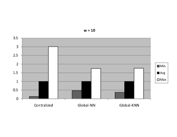
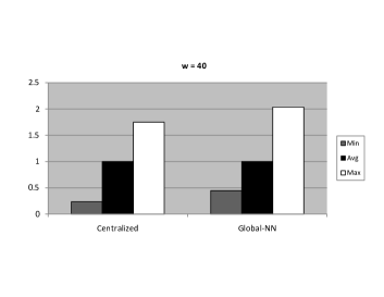
Figure 6: Normalized average, minimum, and maximum amount of energy consumed by a node for global outlier detection.

For the partial information for $w$=40, the normalized range of energy consumption is actually lower for the centralized algorithm than for the distributed one. However, referring back to Figure 5, the average energy consumption for a node in the centralized case is much higher than that for the distributed case. Hence, in this case, the normalized maximum value does not convey the full picture of energy quality of the compared algorithms.

Figure 7: Average transmission and receive energy consumed per node per sample interval vs. $w$ ($n$=4) for localized outlier detection using nearest neighbor outlier detection.

Figure 8: Average transmission and receive energy consumed per node per sample interval vs. $w$ ($n$=4, $k$=4) for localized outlier detection using $k$ nearest neighbor outlier detection.

The plots in Figure 7 compare the rate of energy usage between the centralized algorithm and the distributed algorithm for localized outlier detection. Since the results of using NN and KNN outlier detection methods are nearly identical, only results for the former are shown. Again, the centralized algorithm uses much more energy than the distributed algorithms. Regarding the distributed localized algorithms, the rate of energy usage increases along with the values of epsilon. This is expected since as epsilon increases, so does the message passing overhead as data points travel farther from their place of origin. The behavior of the distributed algorithm in the localized case for nearest neighbor outlier detection is similar to that of global case for the same detection method. Energy usage generally decreases as $w$ increases. As before, we attribute this behavior to the increasing amount of data redundancy as the size of the sliding window increases. In general, the extent of the spatial area over which outliers are defined affects the energy usage trends of the algorithm, but not by a significant amount.

7.2.2 Effect of the number of reported outliers

Figure 9: Average transmission and receive energy consumed per node per sample interval vs. $n$ ($w$=20, $k$=4) for localized outlier detection using k nearest neighbor outlier detection.

We now investigate how the number of outliers produced affects energy usage. Figure 9 shows the plots illustrating the performance of the localized outlier detection algorithms under increasing values for $n$ for KNN outlier detection. Similar plots for NN detection are omitted due to space restrictions and similarity of results; NN detection is negligibly less energy efficient most likely due to a lower rate of convergence. The energy usage trends for these algorithms are straightforward and expected. Energy usage increases along with both $n$ and $epsilon$, which both cause more message passing overhead with increasing value. We also noticed that the rate at which energy usage increased was related to $epsilon$. This is expected since the compounded effects of larger $epsilon$ and $n$ values should make a more noticeable mark on how energy is used.

8 Conclusions

We addressed the problem of unsupervised outlier detection in WSNs. We developed a solution that

1. allows flexibility in the heuristic used to define outliers,

2. computes the result in-network to reduce both bandwidth and energy usage,

3. only uses single hop communication thus permitting very simple node failure detection and message reliability assurance mechanisms (e.g., carrier-sense), and

4. seamlessly accommodates dynamic updates to data.

We evaluated the outlier detection algorithm’s behavior on real-world sensor data using a simulated wireless sensor network. These initial results show promise for our algorithm in that it outperforms a strictly centralized approach under some very important circumstances. When the unabridged data from the entire sensor network are sent to a single location, the node collecting this data as well as its nearest neighbors become a bottleneck of the entire system. Indeed, the density of traffic in this region is proportional to the area of coverage of the entire network while the average node has the traffic density proportional to the area covered by its communication range. In the example that we simulated in the paper, the traffic in the area of the collecting node was about 50 times more dense than in the other parts of the network. The immediate consequence is the shorter life-time of the network, as the nodes near the collecting point will die because of battery exhaustion when many remaining nodes will use just 2% of their energy. The second consequence is the congestion of the traffic that either results in a lot of interference necessitating retransmissions or delays or, alternatively, in delays imposed by a multi-slot bandwidth sharing scheme needed to avoid transmission interference. In short, using the centralized algorithm with its drastic imbalance of the traffic density will put even the best routing protocols under the sever stress. In contrast, our distributed and localized outlier detection algorithms avoid these difficulties.

Our approach is well suited for applications in which the confidence of an outlier rating may be calculated by either an adjustment of sliding window size or the number of neighbors used in a distance-based outlier detection technique. We assert that these applications are critical for resource-constrained sensor networks for two reasons. First, communication is a costly activity motivating the need for only the most accurate data to be transmitted to a client application. Second, emerging safety-critical applications that utilize wireless sensor networks will require the most accurate data, including outliers. This work represents our contribution toward enabling efficient data cleaning solutions for these types of applications.

9 Appendix: Correctness Proofs for the Global Outlier Detection Algorithm

In this section, we provide detailed proofs of Theorems 1 and 2. Before doing so, a few technical lemmas are needed. The first two isolate a couple of useful properties following from the axioms of $R$.

Lemma 1

For any $P\subseteq Q\subseteq D$ where $|P|\geq n$, if $O_{n}(P)$ $\neq$ $O_{n}(Q)$, then there exists $x\in O_{n}(P)$ such that $R(x,P)$ $>$ $R(x,Q)$.

Proof

Assume $O_{n}(P)$ $\neq$ $O_{n}(Q)$. Since $|O_{n}(P)|$ $=$ $|O_{n}(Q)|$ $=$ $n$, then there exists $x\in(O_{n}(P)\setminus O_{n}(Q))$ and $y\in(O_{n}(Q)\setminus O_{n}(P))$. Recall that we assume a tie-breaking machanism is used to ensure $R(.P)$ and $R(.,Q)$ are one-to-one. Thus, by definition of $O_{n}(.)$ it follows that $R(x,P)$ $>$ $R(y,P)$ and $R(y,Q)$ $>$ $R(x,Q)$. The anti-monotoncity axiom implies $R(y,P)$ $\geq$ $R(y,Q)$ yeilding the desired result. ∎

Lemma 2

For any $P\subseteq D$, $x\in O_{n}(P)$, and $z\in P$, we have $R(x,P)$ $=$ $R(x,[P|O_{n}(P)])$ $=$ $R(x,[P|O_{n}(P)]\cup\{z\})$.

Proof

Since, by definition, $[P|x]\subseteq[P|O_{n}(P)]\subseteq([P|O_{n}(P)]\cup\{z\})\subseteq P$, then by the anti-monotonicity axiom it follows that

$$R(x,P) = R(x,[P|x])$$

$$\geq R(x,[P|O_{n}(P)])$$

$$\geq R(x,[P|O_{n}(P)]\cup\{z\})$$

$$\geq R(x,P).$$

∎

The last technical lemma shows that once a sensor $p_{i}$ completes its local computation, then $(D^{i}_{i,j}\cup D^{i}_{j,i})$ contains a particular crucial set of points (among others) needed for consistency among sensors’ outlier estimates.

Lemma 3

For any $p_{i}$, once the main for-loop in the algorithm completes, $[P_{i}|O_{n}(D^{i}_{i,j}\cup D^{i}_{j,i})]$ $\subseteq$ $(D^{i}_{i,j}\cup D^{i}_{j,i})$.

Proof

Let $D^{i}_{i,j}(before)$ denote the set of points held by $p_{i}$ and sent from $p_{i}$ to $p_{j}$ immediately before the execution of the “Repeat unil no change: …” step in the main for loop for $j\in\Gamma_{i}$. For $\ell\geq 1$, let $Z_{j}(\ell)$ denote $Z_{j}$ immediately before the $\ell^{th}$ iteration in the execution of the “Repeat until no change …” step in the main for loop for $j\in\Gamma_{i}$, e.g. $Z_{j}(1)$ $=$ $O_{n}(P_{i})$ $\cup$ $[P_{i}|O_{n}(P_{i})]$.

By definition, $Z_{j}(\ell)$ $\subseteq$ $Z_{j}(\ell+1)$ $\subseteq$ $P_{i}$ and $P_{i}$ is finite. Thus, let $\ell^{*}$ denote the smallest integer such that $Z_{j}(\ell^{*}-1)$ $=$ $Z_{j}(\ell^{*})$. Hence, the “Repeat until no change …” step terminates at the end of iteration $\ell^{*}$ and $Z_{j}=Z_{j}(\ell^{*})$ in the remainder of the main for loop. Therefore,

$$Z_{j}(\ell^{*})=Z_{j}(\ell^{*})\cup[P_{i}|O_{n}(D^{i}_{i,j}(before)\cup D^{i}_{j,i}\cup Z_{j}(\ell^{*}))]$$

and

$$D^{i}_{i,j}\cup D^{i}_{j,i}=D^{i}_{i,j}(before)\cup D^{i}_{j,i}\cup Z_{j}(\ell^{*}).$$

It follows that $[P_{i}|O_{n}(D^{i}_{i,j}\cup D^{i}_{j,i})]\subseteq Z_{j}(\ell^{*})\subseteq(D^{i}_{i,j}\cup D^{i}_{j,i})$. ∎

Now we prove that upon termination of the algorithm, the sensors’ estiamtes are consistent.

Theorem1 Assuming a connected network, if for all sensors $p_{i}$: $D_{i}$ and $\Gamma_{i}$ do not change, then upon termination of the algorithm all sensors’ outlier estimates and supports agree: for all $p_{i},p_{j}$: (i) $O_{n}(P_{i})=O_{n}(P_{j})$ and (ii) $[P_{i}|O_{n}(P_{i})]=[P_{j}|O_{n}(P_{j})]$.

Proof

Since the network is connected, we may assume, without loss of generality, that $p_{i}$ and $p_{j}$ are neighbors. To prove part (i), we will show that $O_{n}(P_{i})$ $=$ $O_{n}(D^{i}_{i,j}\cup D^{i}_{j,i})$ $=$ $O_{n}(D^{j}_{i,j}\cup D^{j}_{j,i})$ $=$ $O_{n}(P_{j})$. The middle equality follows from the fact that $(D^{i}_{i,j}\cup D^{i}_{j,i})$ $=$ $(D^{j}_{i,j}\cup D^{j}_{j,i})$. By symmetry, it suffices to show the first equality.

Suppose $O_{n}(P_{i})$ $\neq$ $O_{n}(D^{i}_{i,j}\cup D^{i}_{j,i})$. The following contradiction is reached. There exists $x\in O_{n}(D^{i}_{i,j}\cup D^{i}_{j,i})$ such that

$$R(x,D^{i}_{i,j}\cup D^{i}_{j,i}) > R(x,P_{i})$$

$$= R(x,[P_{i}|x])$$

$$\geq R(x,[P_{i}|O_{n}(D^{i}_{i,j}\cup D^{i}_{j,i})])$$

$$\geq R(x,D^{i}_{i,j}\cup D^{i}_{j,i}).$$

The first inequality follows from Lemma 1 (with $P$ $=$ $(D^{i}_{i,j}\cup D^{i}_{j,i})$ and $Q$ $=$ $P_{i}$). The equality follows from the definition of support $[.|.]$. The last two inequalities follow from the anti-monotonicity of $R$ and Lemma 3.

To prove part (ii) $[P_{i}|O_{n}(P_{i})]=[P_{j}|O_{n}(P_{j})]$, it suffices to show that for any $x\in$ $O_{n}(D^{i}_{i,j}\cup D^{i}_{j,i})$, it is the case that $[P_{i}|x]$ $=$ $[P_{j}|x]$. This is because $O_{n}(P_{i})$ $=$ $O_{n}(D^{i}_{i,j}\cup D^{i}_{j,i})$ $=$ $O_{n}(P_{j})$. We will prove that $[P_{i}|x]$ $=$ $[P_{i}\cap P_{j}|x]$ $=$ $[P_{j}|x]$. By symmetry it is enough to show the first equality.

From Lemma 3 it follows that

$$[P_{i}|x] \subseteq [P_{i}|O_{n}(D^{i}_{i,j}\cup D^{i}_{j,i})]$$

$$\subseteq (D^{i}_{i,j}\cup D^{i}_{j,i})$$

$$\subseteq (P_{i}\cap P_{j}).$$

Thus, anti-monotonicity implies $R(x,P_{i})$ $\geq$ $R(x,[P_{i}|x])$ $\geq$ $R(x,P_{i}\cap P_{j})$ $\geq$ $R(x,P_{i})$, and so,

$$R(x,P_{i})=R(x,[P_{i}|x])=R(x,P_{i}\cap P_{j}).$$

Therefore, $[P_{i}|x]$, $[P_{i}\cap P_{j}|x]$ are support sets of $x$ with respect to $P_{i}\cap P_{j}$ and $P_{i}$. Since $[P_{i}|x]$ ($[P_{i}\cap P_{j}|x]$) is the unique smallest support set for $x$ with respect to $P_{i}$ ($P_{i}\cap P_{j}$), then it follows that $[P_{i}|x]$ $=$ $[P_{i}\cap P_{j}|x]$. ∎

Finally, we prove that upon termination the sensors’ estiamtes are equal to the correct answer.

Theorem2 Assuming a connected network, if for all sensors $p_{i}$: $D_{i}$ and $\Gamma_{i}$ do not change, then upon termination of the algorithm, all sensors’ outlier estimate will be correct: for all $p_{i}$: $O_{n}(P_{i})=O_{n}(D)$.

Proof

Suppose there exists a sensor $p_{i}$ such that $O_{n}(P_{i})$ $\neq$ $O_{n}(D)$. By Lemma 1 (with $P$ $=$ $P_{i}$ and $Q$ $=$ $D$), there exists $x\in O_{n}(P_{i})$ such that $R(x,P_{i})$ $>$ $R(x,D)$. Moreover, the first equality in Lemma 2 (with $P=P_{i}$) implies that $R(x,[P_{i}|O_{n}(P_{i})])$ $=$ $R(P_{i},x)$.

Since $R(x,[P_{i}|O_{n}(P_{i})])$ $>$ $R(x,D)$, then the smoothness axiom (with $Q_{1}=[P_{i}|O_{n}(P_{i})]$ and $Q_{2}=D$), implies there exists $z\in(D\setminus[P_{i}|O_{n}(P_{i})])$

$$R(x,[P_{i}|O_{n}(P_{i})])>R(x,[P_{i}|O_{n}(P_{i})])\cup\{z\}).$$

This point $z$ must be contained in $P_{j}$ for some sensor $p_{j}$. Hence, the inequality the following contradiction is reached.

$$R(x,[P_{i}|O_{n}(P_{i})]) > R(x,[P_{i}|O_{n}(P_{i})]\cup\{z\})$$

$$= R(x,[P_{i}|O_{n}(P_{j})]\cup\{z\})$$

$$= R(x,[P_{j}|O_{n}(P_{j})])$$

$$= R(x,[P_{i}|O_{n}(P_{i})]).$$

The inequality above leads to the following contradiction. The first equality follows from Theorem 1 part (i). The middle equality follows from the second equality of Lemma 2 (with $P=P_{j}$ and noting that $O_{n}(P_{j})=O_{n}(P_{i})$ by Theorem 1 part (i)). The last equality follows from Theorem 1 part (ii). ∎