Soliton and periodic wave solutions to the osmosis K(2, 2) equation

Abstract

In this paper, two types of traveling wave solutions to the osmosis K(2, 2) equation

$$u_{t}+(u^{2})_{x}-(u^{2})_{xxx}=0$$

are investigated. They are characterized by two parameters. The expresssions for the soliton and periodic wave solutions are obtained.

, ,

1 Introduction

In 1993, Rosenau and Hyman [1] introduced a genuinely nonlinear dispersive equation, a special type of KdV equation, of the form

$$u_{t}+a(u^{n})_{x}+(u^{n})_{xxx}=0,n>1,$$ (1.1)

where $a$ is a constant and both the convection term $(u^{n})_{x}$ and the dispersion effect term $(u^{n})_{xxx}$ are nonlinear. These equations arise in the process of understanding the role of nonlinear dispersion in the formation of structures like liquid drops. Rosenau and Hyman derived solutions called compactons to Eq.(1.1) and showed that while compactons are the essence of the focusing branch where $a>0$, spikes, peaks, and cusps are the hallmark of the defocusing branch where $a<0$ which also supports the motion of kinks. Further, the negative branch, where $a<0$, was found to give rise to solitary patterns having cusps or infinite slopes. The focusing branch and the defocusing branch represent two different models, each leading to a different physical structure. Many powerful methods were applied to construct the exact solutions to Eq.(1.1), such as Adomain method [2], homotopy perturbation method [3], Exp-function method [4], variational iteration method [5], variational method [6, 7]. In [8], Wazwaz studied a generalized forms of the Eq.(1.1), that is $mK(n,n)$ equations and defined by

$$u^{n-1}u_{t}+a(u^{n})_{x}+b(u^{n})_{xxx}=0,n>1,$$ (1.2)

where $a,b$ are constants. He showed how to construct compact and noncompact solutions to Eq.(1.2) and discussed it in higher dimensional spaces in [9]. Chen et al. [10] showed how to construct the general solutions and some special exact solutions to Eq.(1.2) in higher dimensional spatial domains. He et al. [11] considered the bifurcation behavior of travelling wave solutions to Eq.(1.2). Under different parametric conditions, smooth and non-smooth periodic wave solutions, solitary wave solutions and kink and anti-kink wave solutions were obtained. Yan [12] further extended Eq.(1.2) to be a more general form

$$u^{m-1}u_{t}+a(u^{n})_{x}+b(u^{k})_{xxx}=0,nk\neq 1,$$ (1.3)

And using some direct ansatze, some abundant new compacton solutions, solitary wave solutions and periodic wave solutions to Eq.(1.3) were obtained. By using some transformations, Yan [13] obtained some Jacobi elliptic function solutions to Eq.(1.3). Biswas [14] obtained 1-soliton solution of equation with the generalized evolution term

$$(u^{l})_{t}+a(u^{m})u_{x}+b(u^{n})_{xxx}=0,$$ (1.4)

where $a,b$ are constants, while $l,m$ and $n$ are positive integers. Zhu et al. [15] applied the decomposition method and symbolic computation system to develop some new exact solitary wave solutions to the $K(2,2,1)$ equation

$$u_{t}+(u^{2})_{x}-(u^{2})_{xxx}+u_{xxxxx}=0,$$ (1.5)

and the $K(3,3,1)$ equation

$$u_{t}+(u^{3})_{x}-(u^{3})_{xxx}+u_{xxxxx}=0.$$ (1.6)

Recently, Xu and Tian [16] introduced the osmosis $K(2,2)$ equation

$$u_{t}+(u^{2})_{x}-(u^{2})_{xxx}=0,$$ (1.7)

were the positive convection term $(u^{2})_{x}$ means the convection moves along the motion direction, and the negative dispersive term $(u^{2})_{xxx}$ denotes the contracting dispersion. They obtained the peaked solitary wave solution and the periodic cusp wave solution to Eq.(1.7). In [17], the authors obtained the smooth soliton solutions to Eq.(1.7). In this paper, following Vakhnenko and Parkes’s strategy [18, 19] we continue to investigate the traveling wave solutions to Eq.(1.7) and obtain soliton and periodic wave solutions. Our work in this paper covers and extends the results in [16, 17] and may help people to know deeply the described physical process and possible applications of the osmosis K(2, 2) equation.

The remainder of this paper is organized as follows. In Section 2, for completeness and readability, we repeat Appendix A in [19], which discuss the solutions to a first-order ordinary differential equaion. In Section 3, we show that, for travelng wave solutions, Eq.(1.7) may be reduced to a first-order ordinary differential equation involving two arbitrary integration constants $a$ and $b$. We show that there are four distinct periodic solutions corresponding to four different ranges of values of $a$ and restricted ranges of values of $b$. A short conclusion is given in Section 4.

2 Solutions to a first-order ordinary differential equaion

This section is due to Vakhnenko and Parkes (see Appendix A in [19]). For completeness and readability, we state it in the following.

Consider solutions to the following ordinary differential equation

$$(\varphi\varphi_{\xi})^{2}=\varepsilon^{2}f(\varphi),$$ (2.1)

where

$$f(\varphi)=(\varphi-\varphi_{1})(\varphi-\varphi_{2})(\varphi_{3}-\varphi)(\varphi_{4}-\varphi),$$ (2.2)

and $\varphi_{1}$, $\varphi_{2}$, $\varphi_{3}$, $\varphi_{4}$ are chosen to be real constants with $\varphi_{1}\leq\varphi_{2}\leq\varphi\leq\varphi_{3}\leq\varphi_{4}$.

Following [20] we introduce $\zeta$ defined by

$$\frac{d\xi}{d\zeta}=\frac{\varphi}{\varepsilon},$$ (2.3)

so that Eq.(2.1) becomes

$$(\varphi_{\zeta})^{2}=f(\varphi).$$ (2.4)

Eq.(2.4) has two possible forms of solution. The first form is found using result 254.00 in [21]. Its parametric form is

$$\left\{{\begin{array}[]{l}\varphi=\frac{\textstyle\varphi_{2}-\varphi_{1}n\mathrm{sn}^{2}(w|m)}{\textstyle 1-n\mathrm{sn}^{2}(w|m)},\\ \xi=\frac{\displaystyle 1}{\displaystyle\varepsilon p}(w\varphi_{1}+(\varphi_{2}-\varphi_{1})\Pi(n;w|m)),\\ \end{array}}\right.$$ (2.5)

with $w$ as the parameter, where

$$m=\frac{(\varphi_{3}-\varphi_{2})(\varphi_{4}-\varphi_{1})}{(\varphi_{4}-\varphi_{2})(\varphi_{3}-\varphi_{1})},p=\frac{1}{2}\sqrt{(\varphi_{4}-\varphi_{2})(\varphi_{3}-\varphi_{1})},w=p\zeta,$$ (2.6)

and

$$n=\frac{\varphi_{3}-\varphi_{2}}{\varphi_{3}-\varphi_{1}}.$$ (2.7)

In (2.5) $\mathrm{sn}(w|m)$ is a Jacobian elliptic function, where the notation is as used in Chapter 16 of [22]. $\Pi(n;w|m)$ is the elliptic integral of the third kind and the notation is as used in Section 17.2.15 of [22].

The solution to Eq.(2.1) is given in parametric form by (2.5) with $w$ as the parameter. With respect to $w$, $\varphi$ in (2.5) is periodic with period $2K(m)$, where $K(m)$ is the complete elliptic integral of the first kind. It follows from (2.5) that the wavelength $\lambda$ of the solution to (2.1) is

$$\lambda=\frac{\displaystyle 2}{\displaystyle\varepsilon p}|\varphi_{1}K(m)+(\varphi_{2}-\varphi_{1})\Pi(n|m)|.$$ (2.8)

where $\Pi(n|m)$ is the complete elliptic integral of the third kind.

When $\varphi_{3}=\varphi_{4}$, $m=1$, (2.5) becomes

$$\left\{{\begin{array}[]{l}\varphi=\frac{\textstyle\varphi_{2}-\varphi_{1}n\tanh^{2}w}{\textstyle 1-n\tanh^{2}w},\\ \xi=\frac{\textstyle 1}{\textstyle\varepsilon}(\frac{\textstyle w\varphi_{3}}{\textstyle p}-2\tanh^{-1}(\sqrt{n}\tanh w)).\\ \end{array}}\right.$$ (2.9)

The second form of the solution to Eq.(2.4) is found using result 255.00 in [21]. Its parametric form is

$$\left\{{\begin{array}[]{l}\varphi=\frac{\textstyle\varphi_{3}-\varphi_{4}n\mathrm{sn}^{2}(w|m)}{\textstyle 1-n\mathrm{sn}^{2}(w|m)},\\ \xi=\frac{\displaystyle 1}{\displaystyle\varepsilon p}(w\varphi_{4}-(\varphi_{4}-\varphi_{3})\Pi(n;w|m)),\\ \end{array}}\right.$$ (2.10)

where $m,p,w$ are as in (2.6), and

$$n=\frac{\varphi_{3}-\varphi_{2}}{\varphi_{4}-\varphi_{2}}.$$ (2.11)

The solution to Eq.(2.1) is given in parametric form by (2.10) with $w$ as the parameter. The wavelength $\lambda$ of the solution to (2.1) is

$$\lambda=\frac{\displaystyle 2}{\displaystyle\varepsilon p}|\varphi_{4}K(m)-(\varphi_{4}-\varphi_{3})\Pi(n|m)|.$$ (2.12)

When $\varphi_{1}=\varphi_{2}$, $m=1$, (2.10) becomes

$$\left\{{\begin{array}[]{l}\varphi=\frac{\textstyle\varphi_{3}-\varphi_{4}n\tanh^{2}w}{\textstyle 1-n\tanh^{2}w},\\ \xi=\frac{\textstyle 1}{\textstyle\varepsilon}(\frac{\textstyle w\varphi_{2}}{\textstyle p}+2\tanh^{-1}(\sqrt{n}\tanh w)).\\ \end{array}}\right.$$ (2.13)

3 Solitary and periodic wave solutions to Eq.(1.7)

Eq.(1.7) can also be written in the form

$$u_{t}+2uu_{x}-6u_{x}u_{xx}-2uu_{xxx}=0.$$ (3.1)

Let $u=\varphi(\xi)+c$ with $\xi=x-ct$ be a traveling wave solution to Eq.(3.1), then it follows that

$$-c\varphi_{\xi}+2\varphi\varphi_{\xi}-6\varphi_{\xi}\varphi_{\xi\xi}-2\varphi\varphi_{\xi\xi\xi}=0,$$ (3.2)

where $\varphi_{\xi}$ is the derivative of function $\varphi$ with respect to $\xi$.

Integrating (3.2) twice with respect to $\xi$ yields

$$(\varphi\varphi_{\xi})^{2}=\frac{1}{4}(\varphi^{4}-\frac{4c}{3}\varphi^{3}+a\varphi^{2}+b),$$ (3.3)

where $a$ and $b$ are two arbitrary integration constants.

Eq.(3.3) is in the form of Eq.(2.1) with $\varepsilon=\frac{\textstyle 1}{\textstyle 2}$ and $f(\varphi)=(\varphi^{4}-\frac{\textstyle 4c}{\textstyle 3}\varphi^{3}+a\varphi^{2}+b)$. For convenience we define $g(\varphi)$ and $h(\varphi)$ by

$$f(\varphi)=\varphi^{2}g(\varphi)+b,\ \mbox{where}\ g(\varphi)=\varphi^{2}-\frac{4c}{3}\varphi+a,$$ (3.4)

$$f^{\prime}(\varphi)=2\varphi h(\varphi),\ \mbox{where}\ h(\varphi)=2\varphi^{2}-2c\varphi+a,$$ (3.5)

and define $\varphi_{L}$, $\varphi_{R}$, $b_{L}$, and $b_{R}$ by

$$\varphi_{L}=\frac{\textstyle 1}{\textstyle 2}(c-\sqrt{c^{2}-2a}),\varphi_{R}=\frac{\textstyle 1}{\textstyle 2}(c+\sqrt{c^{2}-2a}),$$ (3.6)

$$b_{L}=-\varphi_{L}^{2}g(\varphi_{L})=\frac{\textstyle a^{2}}{\textstyle 4}-\frac{\textstyle 1}{\textstyle 2}c^{2}a+\frac{\textstyle c^{4}}{\textstyle 6}-\frac{\textstyle 1}{\textstyle 6}(c^{3}-2ac)\sqrt{c^{2}-2a},$$ (3.7)

$$b_{R}=-\varphi_{L}^{2}g(\varphi_{L})=\frac{\textstyle a^{2}}{\textstyle 4}-\frac{\textstyle 1}{\textstyle 2}c^{2}a+\frac{\textstyle c^{4}}{\textstyle 6}+\frac{\textstyle 1}{\textstyle 6}(c^{3}-2ac)\sqrt{c^{2}-2a}.$$ (3.8)

Obviously, $\varphi_{L}$, $\varphi_{R}$ are the roots of $h(\varphi)=0$.

Without loss of generality, we suppose the wave speed $c>0$. In the following, suppose that $a<\frac{\textstyle c^{2}}{\textstyle 2}$ and $a\neq 0$ for each value $c>0$, such that $f(\varphi)$ has three distinct stationary points: $\varphi_{L}$, $\varphi_{R}$, $0$ and comprise two minimums separated by a maximum. Under this assumption, Eq.(1.7) has periodic and solitary wave solutions that have different analytical forms depending on the values of $a$ and $b$ as follows:

(1) $a<0$

In this case $\varphi_{L}<0<\varphi_{R}$ and $f(\varphi_{L})>f(\varphi_{R})$. For each value $a<0$ and $0<b<b_{L}$ (a corresponding curve of $f(\varphi)$ is shown in Fig.1(a)), there are periodic loop-like solutions to Eq.(3.3) given by (2.10) so that $0<m<1$, and with wavelength given by (2.12). See Fig.2(a) for an example.

(a)

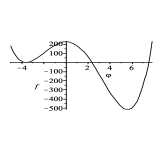
(b)

(c)

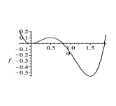
(d)

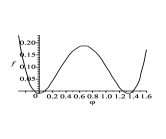
(e)

(f)

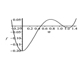
(g)

(h)

Figure 1: The curve of $f(\varphi)$ for the wave speed $c=2$. (a) $a=-40$, $b=200$; (b) $a=-40$, $b=226.0424$; (c) $a=1.5$, $b=-0.05$; (d) $a=1.5$, $b=0$; (e) $a=\frac{\textstyle 16}{\textstyle 9}$, $b=-0.1$; (f) $a=\frac{\textstyle 16}{\textstyle 9}$, $b=0$; (g) $a=\frac{\textstyle 17}{\textstyle 9}$, $b=-0.24$; (h) $a=\frac{\textstyle 17}{\textstyle 9}$, $b=-0.1842$.

The case $a<0$ and $b=b_{L}$ (a corresponding curve of $f(\varphi)$ is shown in Fig.1(b)) corresponds to the limit $\varphi_{1}=\varphi_{2}=\varphi_{L}$ so that $m=1$, and then the solution is a loop-like solitary wave given by (2.13) with $\varphi_{2}\leq\varphi<\varphi_{R}$ and

$$\varphi_{3}=\frac{\textstyle 1}{\textstyle 2}\sqrt{c^{2}-2a}+\frac{\textstyle c}{\textstyle 6}-\frac{\textstyle 1}{\textstyle 3}\sqrt{c^{2}+3c\sqrt{4-2a}},$$ (3.9)

$$\varphi_{4}=\frac{\textstyle 1}{\textstyle 2}\sqrt{c^{2}-2a}+\frac{\textstyle c}{\textstyle 6}+\frac{\textstyle 1}{\textstyle 3}\sqrt{c^{2}+3c\sqrt{4-2a}}.$$ (3.10)

See Fig.3(a) for an example.

(2) $0<a<\frac{\textstyle 4c^{2}}{\textstyle 9}$

In this case $0<\varphi_{L}<\varphi_{R}$ and $f(\varphi_{R})<f(0)$. For each value $0<a<\frac{\textstyle 4c^{2}}{\textstyle 9}$ and $b_{L}<b<0$ (a corresponding curve of $f(\varphi)$ is shown in Fig.1(c)), there are periodic valley-like solutions to Eq.(3.3) given by (2.10) so that $0<m<1$, and with wavelength given by (2.12). See Fig.2(b) for an example.

The case $0<a<\frac{\textstyle 4c^{2}}{\textstyle 9}$ and $b=0$ (a corresponding curve of $f(\varphi)$ is shown in Fig.1(d)) corresponds to the limit $\varphi_{1}=\varphi_{2}=0$ so that $m=1$, and then the solution can be given by (2.13) with $\varphi_{3}$ and $\varphi_{4}$ given by the roots of $g(\varphi)=0$, namely

$$\varphi_{3}=\frac{\textstyle 2c}{\textstyle 3}-\sqrt{\frac{\textstyle 4c^{2}}{\textstyle 9}-a},\varphi_{4}=\frac{\textstyle 2c}{\textstyle 3}+\sqrt{\frac{\textstyle 4c^{2}}{\textstyle 9}-a}.$$ (3.11)

In this case we obtain a weak solution, namely the periodic downward-cusp wave

$$\varphi=\varphi(\xi-2j\xi_{m}),(2j-1)\xi_{m}<\xi<(2j+1)\xi_{m},\ j=0,\pm 1,\pm 2,\cdots,$$ (3.12)

where

$$\varphi(\xi)=(\varphi_{3}-\varphi_{4}\tanh^{2}(\xi/4))\cosh^{2}(\xi/4),$$ (3.13)

and

$$\xi_{m}=4\tanh^{-1}\sqrt{\frac{\varphi_{3}}{\varphi_{4}}}.$$ (3.14)

See Fig.3(b) for an example.

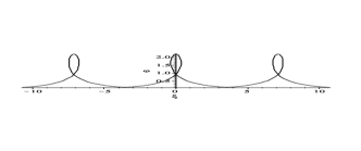
(a)

(b)

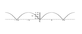
(c)

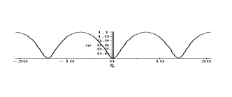
(d)

Figure 2: Periodic solutions to Eq.(3.3) with $0<m<1$ and the wave speed $c=2$. (a) $a=-40$, $b=200$ so $m=0.8978$; (b) $a=1.5$, $b=-0.05$ so $m=0.6893$; (c) $a=\frac{\textstyle 16}{\textstyle 9}$, $b=-0.1$ so $m=0.8254$; (d) $a=\frac{\textstyle 17}{\textstyle 9}$, $b=-0.24$ so $m=0.8412$.

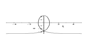
(a)

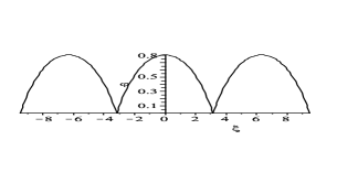
(b)

(c)

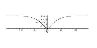
(d)

Figure 3: Solutions to Eq.(3.3) with $m=1$ and the wave speed $c=2$. (a) $a=-40$, $b=226.0424$; (b) $a=1.5$, $b=0$; (c) $a=\frac{\textstyle 16}{\textstyle 9}$, $b=0$; (d) $a=\frac{\textstyle 17}{\textstyle 9}$, $b=-0.1842$.

(3) $a=\frac{\textstyle 4c^{2}}{\textstyle 9}$

In this case $0<\varphi_{L}<\varphi_{R}$ and $f(\varphi_{R})=f(0)$. For $a=\frac{\textstyle 4c^{2}}{\textstyle 9}$ and each value $b_{L}<b<0$ (a corresponding curve of $f(\varphi)$ is shown in Fig.1(e)), there are periodic valley-like solutions to Eq.(3.3) given by (2.5) so that $0<m<1$, and with wavelength given by (2.8). See Fig.2(c) for an example.

The case $a=\frac{\textstyle 4c^{2}}{\textstyle 9}$ and $b=0$ (a corresponding curve of $f(\varphi)$ is shown in Fig.1(f)) corresponds to the limit $\varphi_{3}=\varphi_{4}=\varphi_{R}=\frac{\textstyle 2c}{\textstyle 3}$ and $\varphi_{1}=\varphi_{2}=0$ so that $m=1$. In this case neither (2.9) nor (2.13) is appropriate. Instead we consider Eq.(3.3) with $f(\varphi)=\frac{\textstyle 1}{\textstyle 4}\varphi^{2}(\varphi-\frac{\textstyle 2c}{\textstyle 3})^{2}$ and note that the bound solution has $0<\varphi<\frac{\textstyle 2c}{\textstyle 3}$. On integrating Eq.(3.3) and setting $\varphi=0$ at $\xi=0$ we obtain a weak solution

$$\varphi=-\frac{\textstyle 2c}{\textstyle 3}\exp{(-\frac{\textstyle 1}{\textstyle 2}|\xi|)}+\frac{\textstyle 2c}{\textstyle 3},$$ (3.15)

i.e. a single valley-like peaked solution with amplitude $\frac{\textstyle 2c}{\textstyle 3}$. See Fig.3(c) for an example.

(4) $\frac{\textstyle 4c^{2}}{\textstyle 9}<a<\frac{\textstyle c^{2}}{\textstyle 2}$

In this case $0<\varphi_{L}<\varphi_{R}$ and $f(\varphi_{R})>f(0)$. For each value $\frac{\textstyle 4c^{2}}{\textstyle 9}<a<\frac{\textstyle c^{2}}{\textstyle 2}$ and $b_{L}<b<b_{R}$ (a corresponding curve of $f(\varphi)$ is shown in Fig.1(g)), there are periodic valley-like solutions to Eq.(3.3) given by (2.5) so that $0<m<1$, and with wavelength given by (2.8). See Fig.2(d) for an example.

The case $\frac{\textstyle 4c^{2}}{\textstyle 9}<a<\frac{\textstyle c^{2}}{\textstyle 2}$ and $b=b_{R}$ (a corresponding curve of $f(\varphi)$ is shown in Fig.1(h)) corresponds to the limit $\varphi_{3}=\varphi_{4}=\varphi_{R}$ so that $m=1$, and then the solution is a velley-like solitary wave given by (2.10) with $\varphi_{L}<\varphi\leq\varphi_{3}$ and

$$\varphi_{1}=\frac{\textstyle c}{\textstyle 6}-\frac{\textstyle 1}{\textstyle 2}\sqrt{c^{2}-2a}-\frac{\textstyle 1}{\textstyle 3}\sqrt{c^{2}-3c\sqrt{c^{2}-2a}},$$ (3.16)

$$\varphi_{2}=\frac{\textstyle c}{\textstyle 6}-\frac{\textstyle 1}{\textstyle 2}\sqrt{c^{2}-2a}+\frac{\textstyle 1}{\textstyle 3}\sqrt{c^{2}-3c\sqrt{c^{2}-2a}}.$$ (3.17)

See Fig.3(d) for an example.

4 Conclusion

In this paper, we have found expressions for two types of traveling wave solutions to the osmosis K(2, 2) equation, that is, the soliton and periodic wave solutions. These solutions depend, in effect, on two parameters $a$ and $m$. For $m=1$, there are loop-like ($a<0$), peakon ($a=\frac{\textstyle 4c^{2}}{\textstyle 9}$) and smooth ($\frac{\textstyle 4c^{2}}{\textstyle 9}<a<\frac{\textstyle c^{2}}{\textstyle 2}$) soliton solutions. For $m=1,0<a<\frac{\textstyle 4c^{2}}{\textstyle 9}$ or $0<m<1,a<\frac{\textstyle c^{2}}{\textstyle 2}$ and $a\neq 0$, there are periodic wave solutions.

References

- [1] P. Rosenau, J. M. Hyman, Compactons: solitons with finite wavelengths, Phys. Rev. Lett. 70 (1993) 564-567.
- [2] A. M. Wazwaz, Compactons and solitary patterns structures for variants of the KdV and the KP equations, Appl. Math. Comput. 138 (2003) 309-319.
- [3] J. H. He, Homotopy perturbation method for bifurcation of nonlinear problems, Int. J Nonlinear Sci. Numer. Simulat. 6 (2005) 207-208.
- [4] J. H. He, X. H. Wu, Exp-function method for nonlinear wave equations, Chaos, Solitons and Fractals 30 (2006) 700-708.
- [5] J. H. He, X. H. Wu, Construction of solitary solution and compacton-like solution by variational iteration method, Chaos, Solitons and Fractals 29 (2006) 108-113.
- [6] J. H. He, Some asymptotic methods for strongly nonlinear equations, Int. J Modern Phys. B 20 (2006) 1141-1199.
- [7] L. Xu, Variational approach to solitons of nonlinear dispersive equations, Chaos, Solitons and Fractals 37 (2008) 137-143.
- [8] A. M. Wazwaz, General compacts solitary patterns solutions for modified nonlinear dispersive equation in higher dimensional spaces, Math. Comput. Simulat. 59 (2002) 519-531.
- [9] A. M. Wazwaz, Compact and noncompact structures for a variant of KdV equation in higher dimensions, Appl. Math. Comput. 132 (2002) 29-45.
- [10] Y. Chen, B. Li, H. Q. Zhang, New exact solutions for modified nonlinear dispersive equations in higher dimensions spaces, Math. Comput. Simul. 64 (2004) 549-559.
- [11] B. He, Q. Meng, W. Rui, Y. Long, Bifurcations of travelling wave solutions for the equation, Commun. Nonlinear Sci. Numer. Simulat. 13 (2008) 2114-2123.
- [12] Z. Y. Yan, Modified nonlinearly dispersive equations: I. New compacton solutions and solitary pattern solutions, Comput. Phys. Commun. 152 (2003) 25-33.
- [13] Z. Y. Yan, Modified nonlinearly dispersive equations: II. Jacobi elliptic function solutions, Comput. Phys. Commun. 153 (2003) 1-16.
- [14] A. Biswas, 1-soliton solution of the equation with generalized evolution, Phys. Lett. A 372 (2008) 4601-4602.
- [15] Y. G. Zhu, K. Tong, T. C. Lu, New exact solitary-wave solutions for the and equations, Chaos, Solitons and Fractals 33 (2007) 1411-1416.
- [16] C. H. Xu, L. X. Tian, The bifurcation and peakon for equation with osmosis dispersion, Chaos, Solitons and Fractals 40 (2009) 893-901.
- [17] J. B. Zhou, L. X. Tian, Soliton solution of the osmosis K(2, 2) equation, Phys. Lett. A 372 (2008) 6232-6234.
- [18] V. O. Vakhnenko, E. J. Parkes, Explicit solutions of the Camassa-Holm equation, Chaos, Solitons and Fractals 26 (2005) 1309-1316.
- [19] V. O. Vakhnenko, E. J. Parkes, Periodic and solitary-wave solutions of the Degasperis-Procesi equation, Chaos, Solitons and Fractals 20 (2004) 1059-1073.
- [20] E. J. Parkes, The stability of solutions of Vakhnenko’s equation, J. Phys. A Math. Gen. 26 (1993) 6469-75.
- [21] P. F. Byrd, M. D. Friedman, Handbook of elliptic integrals for engineers and scientists, Springer, Berlin, 1971.
- [22] M. Abramowitz, I. A. Stegun, Handbook of mathematical functions, Dover Publications, New York, 1972.