Deep U-B-V imaging of the Lockman Hole with the LBT

Abstract

Context. We used the large binocular camera (LBC) mounted on the large binocular telescope (LBT) to observe the Lockman Hole in the U, B, and V bands. Our observations cover an area of 925 arcmin². We reached depths of 26.7, 26.3, and 26.3 mag(AB) in the three bands, respectively, in terms of 50% source detection efficiency, making this survey the deepest U-band survey and one of the deepest B and V band surveys with respect to its covered area. We extracted a large number of sources ($\sim 89000$), detected in all three bands and examined their surface density, comparing it with models of galaxy evolution. We find good agreement with previous claims of a steep faint-end slope of the luminosity functions, caused by late-type and irregular galaxies at $z>1.5$. A population of dwarf star-forming galaxies at $1.5<z<2.5$ is needed to explain the U-band number counts. We also find evidence of strong supernova feedback at high redshift. This survey is complementary to the r, i, and z Lockman Hole survey conducted with the Subaru telescope and provides the essential wavelength coverage to derive photometric redshifts and select different types of sources from the Lockman Hole for further study.

Aims.

Methods.

Results.

1 Introduction

The formation and evolution of cosmic structures, such as galaxies, clusters, and the large-scale structure, are some of the most important issues in modern astrophysics. According to hierarchical models, initial fluctuations of the dark matter mass density develop to form galaxies, clusters, and the cosmic web. Such processes leave their footprints in different regimes of the electromagnetic spectrum, and assembling statistically significant samples of extragalactic objects at different wavelengths can give valuable information on the various processes involved in the evolution of the universe.

A very valuable tool for constructing such samples is deep “blind” surveys, where a region in the sky with no bright sources is observed with a long integration time. Optical surveys are very important in this context, as they are able to provide the densest fields in terms of detected sources and serve as “anchor points” for the multi-wavelength coverage. After a multi-wavelength coverage has been achieved, one could apply photometric redshift techniques (e.g. Bolzonella, Miralles & Pelló, 2000; Benítez, 2000; Ilbert et al., 2009) to examine the luminosities of the various sources or select source samples for spectroscopy.

Notable results have been reported in various fields of extragalactic astrophysics using blind deep surveys. Combining imaging and spectroscopic surveys at different regimes of the spectrum, different groups have been able to derive the star formation (e.g. Hopkins, 2004) and accretion histories (e.g. Ueda et al., 2003) of the universe and examine their co-evolution (Vollmer, Beckert & Davies, 2008; Somerville et al., 2008). From optical imaging and photometry alone, one can use the information in the number count of the detected sources to test the geometry and evolutionary models of the universe. For example, Eucledian geometry would result in a constant slope of 0.6 in the galaxy number counts with respect to their magnitudes, but this has been ruled out from early results in this direction (e.g. Gardner, Cowie & Wainscoat, 1993). Measuring the number counts in different wavebands, it is evident that simple geometric models invoking a “deceleration parameter” (q) could not give good fits and some kind of evolution has to be taken into account (Metcalfe et al., 1991). This effect is more severe in blue colours in the form of excess counts at fainter magnitudes and it is widely known as the “faint blue galaxy problem”. With high resolution observations using the HST, Driver et al. (1995) demonstrate that the sources responsible for the faint counts have late-type and irregular morphologies; adding a population of $z\simeq 2$ dwarf star-forming galaxies (Metcalfe et al., 1995) gives a reasonable fit to the blue number counts data. These galaxies contribute to the star formation at redshifts $z\gtrsim 1$ and are merged or simply have evolved to non activity locally.

Support for this scenario comes from the study of the (blue) luminosity functions of different kinds of objects at different redshifts. Ilbert et al. (2005) find that bluer luminosity functions show evidence of more rapid evolution with redshift than redder ones, and later spectral types and bluer colours seem to play a more important role in it (Zucca et al., 2006; Willmer et al., 2006). However, small evolution of the disc population to $z\simeq 1$ is observed by Ilbert et al. (2006), but the strong evolution of bulge-dominated systems could be attributed to a dwarf galaxy population (see also Im et al., 2001). The study luminosity function is limited to relatively bright objects as it is based on redshifts. A number count distribution can probe fainter objects and give an approximation on the faint-end slope (Barro et al., 2009) of the LF and help distinguish between different results (see comparisons in Ilbert et al. 2005 and Zucca et al. 2006). In this paper we present deep U-B-V band observations of the Lockman Hole with the corresponding number counts to 27.5 mag(AB).

2 The Lockman Hole multi-wavelength survey

The Lockman Hole is a region with minimal galactic absorption ($N_{\rm HI}=4.5\times 10^{19}\,{\rm cm}^{-2}$, Lockman, Jahoda & McCammon, 1986) and the absolute minimum of infrared cirrus emission in the sky. Its position in the northern sky ($\alpha=10^{\rm h}52^{\rm m}43^{\rm s}$, $\delta=57^{\circ}28\arcmin 48\arcsec$) makes it an ideal location for deep surveys. Indeed it has a large multi-wavelength coverage spanning from X-rays to meter-wavelength radio. In X-rays it has been observed with the ROSAT satellite (Hasinger et al., 1998) and more recently with XMM (Hasinger et al., 2001; Brunner et al., 2008), reaching a depth of $1.9\times 10^{-16}\,{\rm erg}\,{\rm cm}^{-2}\,{\rm s}^{-1}$ in the 0.5-2.0 keV band. In the ultra-violet it has been observed by GALEX (Martin et al., 2005) as one of its deep fields, with the data being publically available. In the near infrared (J and K bands) it is a part of the UKIDSS ultra deep survey (Lawrence et al., 2007) reaching K$\sim$23(AB). In infrared wavelengths it was observed by ISO using both ISOPHOT and ISOCAM (Kawara et al., 2004; Fadda et al., 2004; Rodighiero et al., 2004) and more recently there have been observations with Spitzer-IRAC (Huang et al., 2004) and Spitzer MIPS (Egami et al., 2008). The Lockman Hole is also part of the SWIRE survey (Lonsdale et al., 2003), observed with both IRAC and MIPS and covering a much wider (but shallower) area. There have been a number of millimeter - sub-mm observations of the Lockman Hole, namely with the JCMT-SCUBA (Coppin et al., 2006), JCMT-AzTEC (Scott et al., 2006), IRAM-MAMBO (Greve et al., 2004), and CSO-Bolocam (Laurent et al., 2005). In the radio regime, the Lockman Hole has been observed with the VLA, both in 5 and in 1.4 GHz (Ciliegi et al., 2003; Ivison et al., 2002; Biggs & Ivison, 2006) and with MERLIN in 1.4 GHz (Biggs & Ivison, 2008). Finally, in meter-wavelengths it was targeted by the GMRT (Garn et al., 2008).

In this work we present the results of an imaging campaign of the Lockman Hole in the optical. We have used the LBT to obtain deep U, B, and V images. The “red” part of the optical imaging campaign has been conducted with the Subaru telescope (in the r, i, and z bands) and will be presented by Szokoly et al. (in preparation).

3 Observations

The observations were made with the Large Binocular Camera (LBC, Giallongo et al., 2008) of the Large Binocular Telescope (LBT) on Mount Graham, Arizona. The LBT has two 8.4 m mirrors on a common mount and both of them are equipped with a prime focus camera. Both LBCs contain four CCD chips with 2048$\times$4608 pixels each. Three chips are aligned parallel to each other while the fourth is tilted by 90 degrees and located above them. This provides a 23$\times$23 arcmin field of view with a sampling of 0.23 arcsec/pixel. The gaps between the CCDs are 945 nm wide, which corresponds to 18 arcsec, thus a 5-point circular dither pattern with a diameter of 30 arcsec was chosen to provide good coverage over the whole area.

Both cameras have an 8 position filter wheel each, and together a total of 13 filters are available, covering a range from the ultraviolet to the near-infrared. For the U-band Lockman Hole imaging we used the special LBT U-band filter (see Fig. 1) which has a more uniform coverage and better efficiency than the standard U-Bessel. For the other images we used the standard B-Bessel and V-Bessel filters.

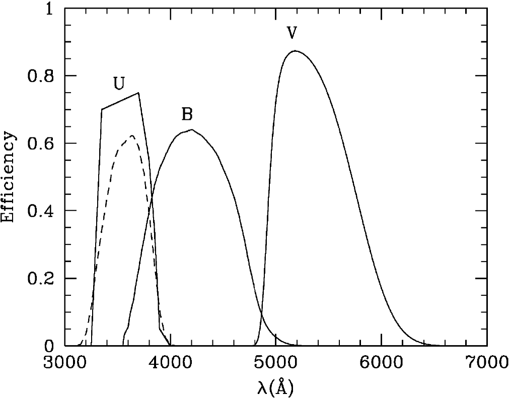
Figure 1: Transmission curves of the filters used (U-spec - B-Bessel - V-Bessel) are shown by continuous lines. The dotted line represents the U-Bessel filter available on the LBC. We have chosen the U-spec filter for the U-band on grounds of its better efficiency and more uniform spectral coverage. These curves represent the filters’ responses without accounting for the detectors’ responses or the atmosphere. The detectors’ responses are slightly different for the two arms of the telescope which might have an effect in the V-band.

The Lockman Hole was observed in March, April and May 2007 during science demonstration time (SDT; PI: E. Egami), when only the camera on the “blue” channel of the telescope was available, and in 2008 and 2009 during LBTB (German institutes’) time (PI: G. Hasinger) with both cameras available in “binocular” mode. We have chosen 2 different pointings as centres of the image, corresponding to the VLA ($\alpha=10^{\rm h}52^{\rm m}08.8^{\rm s}$, $\delta=57^{\circ}21\arcmin 34\arcsec$, Ivison et al. 2002) and the XMM ($\alpha=10^{\rm h}52^{\rm m}43^{\rm s}$, $\delta=57^{\circ}28\arcmin 48\arcsec$, Hasinger et al. 2001) pointings. These are separated by 8.6 arcmin, so there is a large area of overlap, where our images have the highest sensitivity. During the science demonstration time the observing time was split in half between XMM and VLA exposures and during the LBTB time we concentrated on the XMM area.

The total time spent on the Lockman Hole was 36.8 hours which are distributed among the various filters using both channels (when available) as described in Tab. 1. The exposure time for each observation was 360 seconds initially, but it was reduced to 180 seconds for later observing runs (May 2008 onwards), after discovering a large number of saturated sources and limited source tracking efficiency of the telescope for long exposures. The effective exposure time however is as observational problems such as high altitude cirrus clouds or bad seeing diminish the quality of certain images which were not used for creating the final stacks. As seen from Tab. 1 the time efficiency of the three bands is in the order of 65%.

We should note here that the V-band observations were taken using both the blue and the red arms of the telescope. The blue arm was used during SDT, and the red during LBTB time. Although the response curves of the two V-band filters are identical, the quantum efficiencies of the detectors are slightly different. For the analysis presented in this paper this effect is not significant and we merge the two ($V_{b}$ and $V_{r}$) images to achieve greater depth. However in more detailed studies, one should treat the $V_{b}$ and $V_{r}$ images separately.

		U	B	V
SDT	21 February 2007		60
	23 February 2007		30
	25 February 2007		60
	15 March 2007			54
	16 March 2007			114
	02 April 2007		30
	11 April 2007	30	30
	10 May 2007	60
	11 May 2007	54
	12 May 2007	54
	19 May 2007	90
	20 May 2007	60
	21 May 2007	36
	22 May 2007	60
	11 June 2007	60
LBTB	07 March 2008	90	120	120
	08 May 2008	168
	09 May 2008	78
	11 May 2008	240
	29 December 2008		60	60
	30 December 2008	60	54	30
	31 December 2008	63
	01 March 2009		69	69
	02 March 2009	51
SDT		504	210	168
LBTB		750	303	279
Total		1254	513	441
Effective		828	333	321

Table 1: Details of the observing runs (time is in minutes). The SDT runs were made using the blue channel only, whereas the LBTB runs used both telescopes. The effective exposure time is the time actually used for the final stacks.

4 Data reduction

For the reduction of the data we have primarily used IRAF routines included in the mscred package, which is designed to reduce mosaic data.

4.1 Initial calibration

Initial corrections to remove the “pedestal” level of each chip have been carried out using the overscan regions. We have found that the level of the corrections varies significantly (up to 5%) with the column of the chip and therefore we fitted an 8-order Legendre polynomial to it. Residual errors (possibly row-dependent) have been corrected using bias frames taken at the beginning and end of each night with zero integration time.

Flat corrections have been made using sky flat frames taken at either dusk or dawn (or both) for each filter at each arm of the telescope separately. A master flat has been created for each night, filter, and arm. We divided the bias-corrected images with their respective flat fields and noticed that the outer edges of the fourth chip, corresponding to the outer edges of the field of view were extremely noisy, possibly due to poor illumination. We flagged them as bad regions.

After flat-fielding, we corrected the images for bad pixels. These include columns of the CCD with non linear response or dust on the CCD surface. Bad pixel masks are created and the correction has been made by interpolating the values of neighboring pixels. Note that because of the absence of neighboring pixels on the edges of the field of view, these areas are not corrected and are simply not taken into account for the final stages when the images are stacked.

Finally, there are some bright sources in the field which saturate the response of the CCD. In the most severe cases the flux is so high that the current affects the neighboring pixels, leaving “bleeding trails”. This has a significant effect to the B and V images and therefore these regions have been identified and masked out.

4.2 Astrometry

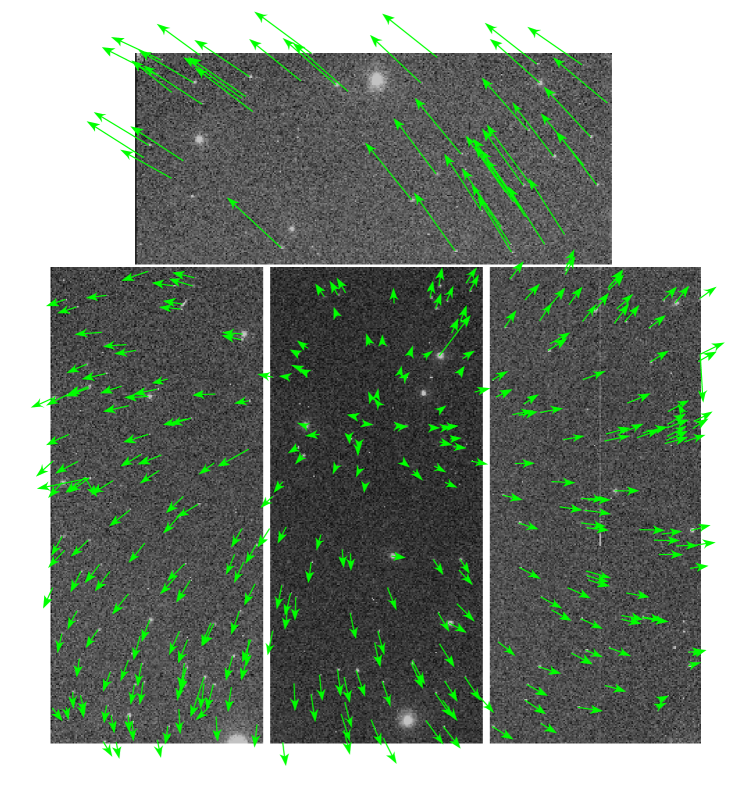
Figure 2: Astrometrical solutions applied to an exposure image of 11 June 2007 (U-band). The image has been bias and flat calibrated but no astrometrical solution has been applied. The arrows represent the shifts to the calibration sources exaggerated 8 times. To compensate for the distortion we dealt with each chip separately and after applying an initial shift we fitted a 4th order polynomial to the corrections. The corrected images have an rms scatter of $\sim$0.2 arcsec

Before dealing with the (arcsecond-scale) astrometric errors, we correct each image for an initial offset, in the order of several arseconds, caused by the telescope’s pointing inaccuracy. We use the brightest ($r<19$) sources from the USNO-A2 (Monet, 1998) catalogue to correct for this offset. This is done by simply updating the wcs header of each file to match the coordinates of the catalogue stars.

After having done that, we need to correct for the true astrometric errors caused by the camera distortion. For this purpose we do not use the USNO catalogue of the brightest stars, as proper motions could have an effect in the solutions we derive. We use an astrometry corrected catalogue of the Lockman Hole, which includes sources brighter than $V=19$. This is based on observations made with the Canada-France-Hawaii Telescope (CFHT, e.g. Wilson et al., 2001) and the data reduction details are in Kaiser et al. (1999). The absolute astrometry of this catalogue is based on USNO-A2 which claimed accuracy is 0.25 arcsec (Monet, 1998).

To apply detailed astrometrical solutions we deal with each chip separately in order to avoid fitting for jumps between the chips. We first apply a distortion pattern which we empirically derived by correcting a random image and then fit a 4-order polynomial to each direction of each chip. The final rms scatter we get is in the order of  0.2 arcsec. An example of the astrometrical solutions applied (after correcting for the overall pointing offset) is given in Fig. 2. To measure the final astrometrical accuracy, we compare our LBT images with the USNO-A2 catalogue (see Fig. 3) and with others, such as USNO-B1, APM (Irwin et al., 1994), SWIRE-IRAC(3.2$\mu$m) (Lonsdale et al., 2003) and L-band VLA (Biggs & Ivison, 2006). Their positions typically agree within 0.4 arcsec and the typical standard deviation is 0.45 arcsec, which is the value we assume to be our final astrometric accuracy. The relative astrometry of the U-B-V images based on the positions of bright ($<$24 mag) and realtively compact (FWHM$<$1.5 arcsec) sources has a standard deviation of 0.066 ″.

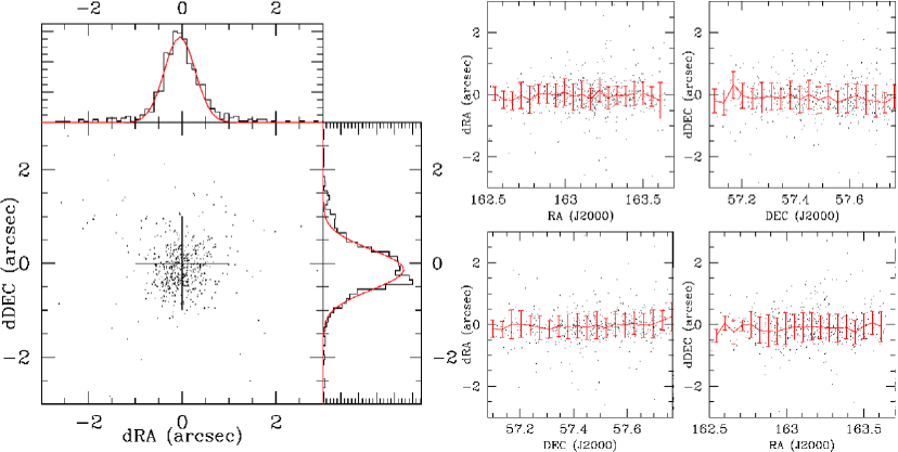
Figure 3: Final astrometry check using the USNO-A2 catalogue. The left panel shows the RA and DEC differences between the LBT and USNO counterparts. The (gaussian) fits to the respective histograms have $\sigma=0.47$ arcsec and $\sigma=0.59$ arcsec for RA and DEC and the means are at -0.06 arcsec and -0.13 arcsec respectively. The right panels show the RA and DEC differences across the entire LBT image, where we do not observe any systematic trends.

4.3 Background subtraction

The final step is to subtract the sky background. After having flattened the images and having corrected for field distortions (without preserving the flux of each pixel) the sky background is uniform within a good approximation. To subtract it we fragment the image to a grid constructed of 100x100 pixel wide meshes and smooth each mesh by a median filter with a 5x5 pixel kernel using sextractor (Bertin & Arnouts, 1996). We chose this method over fitting a function to the background because it gives better results in the vicinity of bright stars in the sense that it does not over-correct the background.

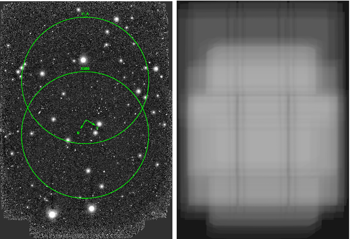
Figure 4: Final U-band image and corresponding exposure map. The image covers both the XMM and the VLA fields, which are marked with 10′-radii circular regios, close to their typical widths. The highest exposure is in the overlapping region between them.

After having subtracted the background, we re-project the four chips of each image to a common frame, applying the complex astrometrical solutions. By doing that we get rid of complex headers and multiple frame images. We use the same reference image to re-project all images in all filters. Finally, after removing any bad images due to poor observing conditions or other problems, we stack all the images (weighted according to their exposure times) to produce the U, B, and V maps of the Lockman Hole. An example image (in the U band) and its corresponding exposure map is shown in Fig. 4. The regions mark the deep VLA and XMM surveys with 10′radii, which are their typical widths.

4.4 Flux calibration

For the B and V filters we rely on flux-calibrated images of the Lockman Hole taken with the Calar Alto Telescope (see Kaiser et al., 1999; Wilson et al., 2001). We select point-like sources which are not saturated in any of the images and conduct aperture photometry. We compare the results and derive zero-point magnitudes for our final images. We do not find evidence for a gradient across the image.

As there are no sources with known magnitudes in the U-spec band, we had to rely on U-Bessel standards to derive the zero-point offsets. We used the observations of June 11, 2007 when standard stars are observed with both the U-Bessel and the U-spec filters. We have applied the same calibration (bias subtraction and flat fielding) using the same bias and flat-field images to all the target and standard star frames and did not perform any astrometric corrections nor we combined the calibrated files. We measured the observed magnitudes of four standard stars without applying any zero-point offsets and found a difference of $\sim 0.67$ mag. We attribute this difference to the higher efficiency of the U-spec filter, as the spectral profiles are similar.

We then calculate the zero-point offset for the U-Bessel filter using the equation:

$$U_{Bessel}[zp]=U_{Bessel}-u_{Bessel}-k_{U}X-c.t.(U-B)$$

where $U_{Bessel}$ and $u_{Bessel}$ are the correct and observed magnitudes, $k_{U}$ is the extinction term for the U-Bessel filter, $X$ the airmass of the observation and c.t. the colour term. To have consistency between the different observations made with different integration times, we have adopted everything to $t_{int}=1$ s. During the commissioning of the LBC-blue the extinction term for the U-Bessel filter was measured to be $k_{U}=-0.48\pm 0.02$ and the colour term $c.t.=0.036$. Applying the $U_{Bessel}$, $u_{Bessel}$, and $X$ values of the standard stars we derive: $U_{Bessel}[zp]=(26.012\pm 0.014)-2.5\log\frac{t_{\rm exp}}{1{\rm sec}}$.

To calculate the U-spec zero-point offset we shift the value of the U-Bessel offset by the mean measured magnitude difference of the standard stars. This is the equivalent of assuming that the standard stars have the same magnitudes in the U-spec and U-Bessel filters. The central wavelengths and widths of the two filters are very similar, so such an assumption does not affect the result in great extent. We find: $U_{spec}[zp]=26.073\pm 0.012$.

To calculate the zero-point offset of the final image, where as a result of rescaling of the individual images and combining them the connection to the original gains has been lost, we use the number mentioned in the previous paragraph to derive the magnitudes of Lockman Hole sources using the raw images. For this purpose we selected 43 non saturated sources with almost gaussian profiles which are observed with the second chip of the mosaic, as the standard stars. We use these 43 sources to measure the zero-point magnitude of the final combined image. We derive $zp_{final}=32.041\pm 0.013$ and do not find any evidence for a gradient in any direction of the image. The magnitudes of the standard stars are given in the Landolt photometric system (Landolt, 1992) which is based on Vega magnitudes. We use U-Bessel AB correction calculated during the commissioning time (0.87), so our final zero-point offset for the U band is: $U_{spec,AB}[zp]=32.911\pm 0.013$.

Detailed information on the three (U-B-V) final images can be found in Tab. 2.

	zero-point	seeing	number	50% eff.	4.5 $\sigma$
	(AB mag)	(arcsec)	of sources	(AB mag)	(AB mag)
U	32.911	1.06	51500	26.7	28.9
B	33.830	0.94	76071	26.3	29.1
V	34.110	1.03	68278	26.3	28.6

Table 2: Flux calibration, quality and source extraction information of the images.

5 Results

5.1 Source catalogues

The source detection has been done independently in each of the U-B-V images using sextractor. Sources are identified as regions where 12 or more adjacent pixels have values above 1.2 times the local background rms. The algorithm first subtracts the background which is fitted by segmenting the image with a grid. If the grid is too fine, a fraction of the flux of the sources will be subtracted as background and this will be more severe for extended sources. On the other hand, a very large mesh will fail to subtract the background near very bright objects, where stray light contaminates the image, so the source extraction will fail in these areas. To overcome these issues we ran sextractor in two steps: first we used a very fine grid (with a $5\times 5$ pixel mesh) to subtract the background and created a “source detection” image. We then re-run sextractor in dual mode using this image to detect the sources but measure their fluxes from the original image, where the background is subtracted using a $10\times 10$ pixel mesh.

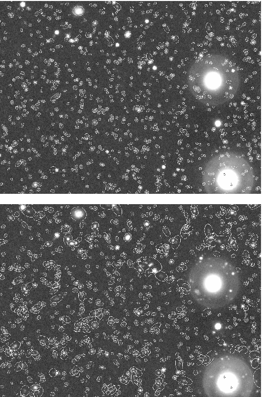
Figure 5: Apertures of extracted sources in the U image. The upper panel shows the “dual mode” results and the lower the “single mode” (see text) Note that the detection efficiency near the bright object as, the deblending efficiency and the apertures of faint sources are much better in “dual mode”, but the apertures of bright objects are more reasonable in “single mode”.

This method has the drawback that the apertures where we measure the flux are too tight for bright sources, which appear more extended in the images and as a consequence we are losing a fraction of their flux (see Fig. 5, upper panel). Therefore we run sextractor once more in “single mode” (with a $10\times 10$ pixel mesh for the background; see also Fig. 5, lower panel) and replace the sources with magnitudes brighter than 22 of the original catalogue with those extracted in “single mode”.

Finally, in order to avoid spurious detections, we remove from our catalogues sources whose isophotal flux errors are larger than the fluxes and therefore do not have reliable photometry and sources whose FWHM is less than 90% of the seeing of each image (1.06, 0.94, and 1.03 arcsec for the U, B, and V images respectively) and are related with imaging artifacts. We also optically inspect the remaining sources and remove obvious false detections related with bad pixels, dust on the CCDs, bleeding trails etc as well as saturated sources. The final U, B, and V catalogues contain 51500, 76071, and 68278 sources respectively.

In order to estimate the detection limits of our catalogues we plot the flux error against the flux of each detected source (see Fig. 6). We do this because we used a more complex selection algorithm to extract sources than a simple signal-to-noise cut. The dashed lines in Fig. 6 represent signal-to-noise ratios of 1, 2, and 3 from left to right and the red line the (empirical) “detection limit”. We notice that the faintest sources tend to be closer to this limit and this is a result of them being point-like. The resulting detection threshold magnitudes and signal-to-noise ratios (see Tab. 2) are not detection limits in the sense that sources with fluxes (or SNRs) above these limits are detected, they are indicative of the sensitivity of the survey representing the lowest flux (and respective SNR) of securely detected sources. They also provide no information on the completeness of the survey at a given flux (or SNR), nor an estimation of the chance of a spurious detection. Such an analysis is described in §5.3.

Figure 6: Flux error versus flux diagrams for source detections in the U, B, and V filters. The zero-point magnitudes for the three filters are $32.911\pm 0.013$, $33.830\pm 0.014$, and $34.110\pm 0.011$ respectively. The dashed lines represent signal-to-noise ratios of 1, 2, and 3, and the red solid lines represent the (empirical) limit of the source extracting algorithm used ($4.5\,\sigma$). The horizontal and vertical solid lines mark the minimum flux and the respective minimum flux error of the faintest sources extracted. The dotted and dash-dotted lines mark the 50% efficiency limit and the limit of the number count analysis respectively.

5.2 Colours

To create colour catalogues of the various sources detected in the U, B, and V images, one could simply cross-correlate the three source catalogues described in the previous paragraphs and compare the fluxes in the different bands. This however would introduce an uncertainty on the choice of the best counterpart and moreover the deblending efficiency of sextractor varies between the different images, so a source in one catalogue might be blended with a close pair in another or vice-versa. Therefore we chose to select one image to extract the sources and then measure their fluxes using the other images in dual mode.

We make the source detection on a combined image of the three bands, the $\chi^{2}$-image. The PSFs of the three images we combine do not have significant differences; the worse PSF (U-band) is only 6% larger than the best (B-band), therefore we do not lose in quality when combining the images as compared to using the best PSF image and we gain in S/N. We follow the recipe of Szalay, Connolly & Szokoly (1999) to create the $\chi^{2}$-image: after carefully removing any residual background of each image (using the “-BACKGROUND” checkimage option of sextractor) we fit the off-source pixel histogram with a gaussian, checking that the noise profile is indeed gaussian. We then scale the three images according to their noise amplitudes and we create the $\chi^{2}$-image, which is the square root of the sum of the squares of the individual pixel values. We then extract the sources from the combined image using the method described in the previous paragraph and measure the fluxes in the individual U-B-V images. Again, we consider a detection real if its FWHM is $>90\%$ of the PSF FWHM of the best individual image (0.85 arcsec). The final colour catalogue contains 88429 with detections in all three bands.

A colour-colour ($U-B$ vs. $B-V$) diagram of the Lockman Hole sources is shown in Fig. 7. The greyscale represents the density of sources detected in all three bands and the black lines mark the selection area of $z\gtrsim 3$ objects. We also calculate the colours of different galaxy SED templates from Coleman, Wu & Weedman (1980) and a QSO template from Cristiani & Vio (1990). The galaxy templates are extrapolated to the Lyman break (911.25 Å) and are zeroed thereafter. The Lyman break meets the blue end of the U filter at $z=2.5$ and this is the highest redshift where the colour tracks are reliable (solid lines). The dotted lines $(z>2.5)$ are shown as an approximation of the colours of high redshift galaxies.

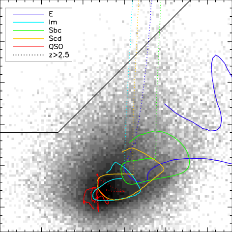
Figure 7: Optical colours of the Lockman hole sources in the AB system. THe greyscale represents the density of sources detected in all three bands are plotted. The black line marks the selection area of U-dropout sources with redshift $z\gtrsim 3$ (see Fig. 12 and § 6.2). Dotted are the tracks above $z=2.5$, where the SEDs are not well sampled. The coloured lines represent tracks of different SED templates: blue line for ellipticals, cyan for irregular, green for Sbc, yellow for Scd, and red for QSO.

5.3 Number counts

In order to derive the differential number counts of extragalactic sources in the U, B, and V bands, we select a region in the centre of the field with uniform exposure within a good approximation. This region has a size of $14\times 13.3$ arcmin and is located in the area where the XMM and VLA observations overlap.

The first step in calculating number counts is to estimate the source extracting efficiency at a given magnitude. The way to do it is to create an image with artificial sources of known magnitudes and to apply the same source extracting procedure as applied to the image, and measure the fraction of the sources recovered. We use the artdata package in IRAF to create lists of artificial sources. They contain sources with a uniform spatial distribution and magnitudes ranging from 16 to 29 following a power-law distribution with a power of 0.5. The surface brightness profiles are exponential discs (resembling spirals) and $r^{-1/4}$ discs, resembling ellipticals. The fraction of elliptical galaxies in the random catalogues is 20% (see van den Bergh, 2001). Here, we caution that adding a large number of artificial sources in the image might change its crowding properties, however we need a large sample of sources for reliable statistics. To avoid confusion, we create a list of 100000 sources and split it to 100 1000-source samples.

We plant these sources into the cutouts of the final images and apply the same source extracting algorithm we used to create the source catalogues. We then measure the fraction of the artificial catalogue we retrieve, hence the efficiency of the source detecting method at any given magnitude and average the results of the 100 subsamples. Increasing the number of sources of each subsample we get similar results up to the point where the number of sources is comparable to the number of “real” sources in the region ($\sim 10000$). The results for all three bands are shown in Fig. 8. This method has the drawback that the artificial sources are mixed with real sources, and so there is no way of knowing whether a detected source is real or an artifact. The surface density of sources with magnitude (at any band) $<27$ is close to $2\times 10^{5}\rm{deg}^{-2}$, which means that there is a $\sim 10$% probability that a real source is within 1.5 arcsec of a random position.

To measure the spurious source detection rate we measure the off-source noise of the science images and check that the noise profile is gaussian. We then create gaussian noise maps of the same amplitude and insert the artificial sources there. In this case it is desirable to reproduce the crowding of the original field, so we include a large number of artificial sources (30000), which is the number of sources with magnitude $<29$ we expect in this field. The source extraction output to these composite images provides the information of the spurious detection rate, plotted with the red lines in Fig. 8. We can see that the number of spurious sources is negligible below 26.5 mag and starts becoming important above 28.0 mag, where the efficiency drops to practically unusable values. From these diagrams we can also derive the magnitude where the detecting efficiency drops below 0.5, which is a meaningful measure of the detection threshold of the image. This threshold is 26.7 mag(AB), 26.3 mag(AB), and 26.3 mag(AB) for the U, B, and V bands respectively.

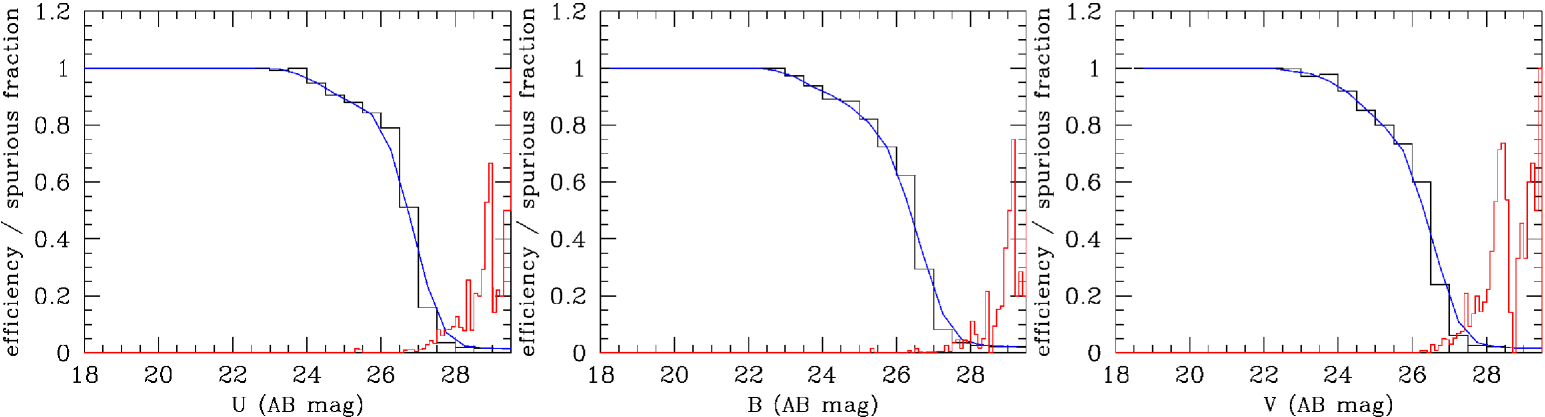
Figure 8: Detection efficiency histograms of the source detection algorithm used, derived from simulations. The blue lines represent the smoothed efficiencies used to correct the surface density distributions. The red histograms are the estimates of the fraction of detections which are spurious, using the artificial noise images.

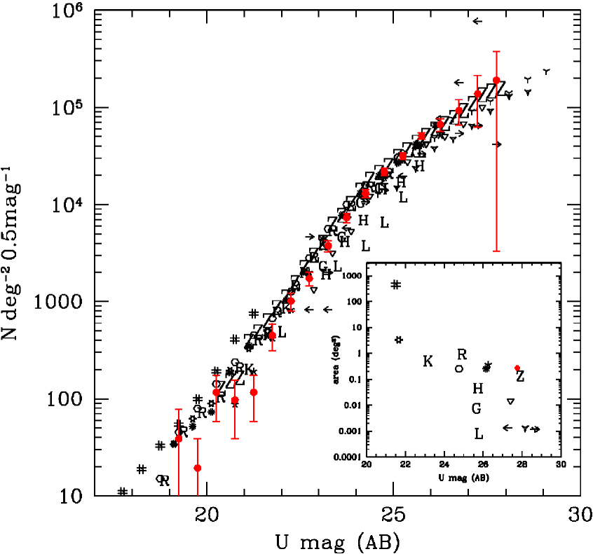
Figure 9: U-band surface density distribution corrected for efficiency and spurious detections. The data points of this study (seen in Tab. 4) are plotted in red dots, while various symbols represent the results of other surveys found in the literature (see Tab. 3), corrected to AB magnitudes. The inner plot shows the depth of each survey (in terms of secure number count measurements) with respect to its width.

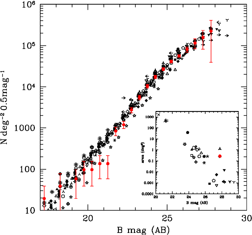
Figure 10: Same as Fig. 9 but for the B-band

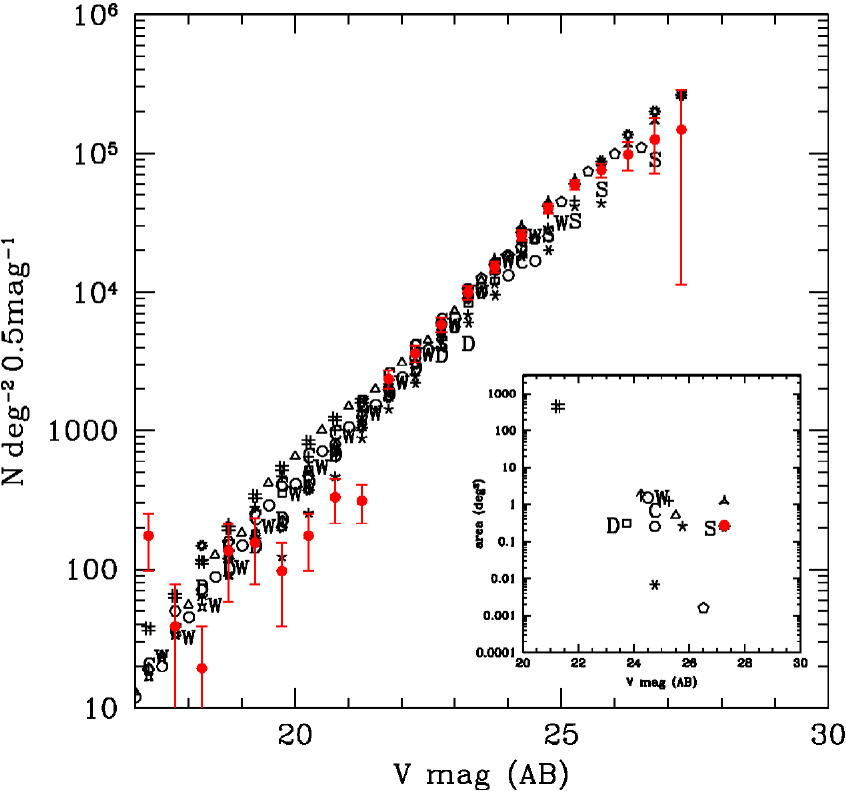
Figure 11: Same as Fig. 9 but for the V-band

Figures 9-11 show the surface density distributions for the three bands observed. Data points of other studies found in the literature are also plotted. We have binned the magnitudes of the observed sources in bins of 0.5 mag. For each bin we corrected the source counts using the efficiency and spurious detection information. As we are interested in galaxy counts, we need a selection mechanism for stellar sources, and as such we use the “stellarity index” of sextractor. This estimate works well for bright sources, but because fainter galaxies can appear point-like it fails for larger magnitudes. As a limiting magnitude we choose 21.5(AB). Below this limit the stellar counts are anyway negligible with respect to the number of galaxies (see e.g. Jarrett, Dickman & Herbst, 1994). The error bars take into account Poisson uncertainties of the uncorrected counts, efficiency uncertainties and cosmic variance. For the latter we use the computational tool of Trenti & Stiavelli (2008), which compares the two-point correlation function of dark matter with the volume of the survey. As a typical redshift for our survey we use $z=1$ (see also §6.1), though using a different value in the range $0.5-2.5$ does not change the result in great extent. We find that the cosmic variance uncertainty is important for bright magnitudes (typically $<25.5$) where the number of intrinsic objects is relatively small. For fainter magnitudes the efficiency uncertainties dominate. As an estimation of those we choose the mean efficiency difference between the bin in question and its neighboring bins. This way we account for the effects of binning, in other words the different efficiencies the magnitudes within each bin have.

Reference	Symbol	Telescope	Instrument
Alcalá et al. (2004)	$\triangle$	ESO/MPG 2.2 m	WFI
Arnouts et al. (1997)	$\Box$	ESO 3.60 m	EFOSC
		ESO-NTT 3.5 m	EMMI
Arnouts et al. (1999)	$\pentagon$	ESO-NTT 3.5 m	SUSI
Arnouts et al. (2001)	$\hexagon$	ESO/MPG 2.2 m	WFI
Berta et al. (2006)	$\Circle$	ESO/MPG 2.2 m	ESIS
Bertin & Dennefeld (1997)	$\Yup$	CERGA 0.9 m	d-MAMA
		ESO
		SERC
Cabanac et al. (2000)	C	CFHT	UH8K
Capak et al. (2004)	$\APLstar$	Subaru	Suprime
Driver et al. (1994)	$\hexstar$	WHT	Hitchhiker
Drory et al. (2001)	D	Calar Alto 2.2 m	CAFOS
Eliche-Moral et al. (2006)	✹	INT La Palma	WFC
Heydon-Dumbleton et al. (1989)	$\times$	UKST	d-COSMOS
Furusawa et al. (2008)	C	Subaru	Suprime
Gardner et al. (1996)	✧	KPNO 0.9 m	T2KA
Grazian et al. (2009)	Z	LBT	LBC
Guhathakurta et al. (1990)	G	CTIAO	pr. focus CCD
Hogg et al. (1997)	H	Hale Telescope	COSMIC
Huang et al. (2001)	✩	Calar Alto 2.2 m	CCD camera
		Calar Alto 2.5 m
Jones et al. (1991)	B	AAT	pr. focus d-COSMOS
Kashikawa et al. (2004)	F	Subaru	Suprime
Koo (1986)	K	KPNO 4 m	photographic plates
Kümmel et al. (2001)	$\blacktriangle$	Calar Alto 3.5 m	Cassegrain CCD
Lilly et al. (1991)	$\blacksquare$	CFHT	NSF1-TI
		UH 2.2 m
Liske et al. (2003)		INT La Palma	WFC
Maddox et al. (1990)	D	UKST	d-APM
McCracken et al. (2001)	$\Diamond$	CFHT	UH8K
McCracken et al. (2003)	$+$	CFHT	CFH12K
Metcalfe et al. (1991)	✧	INT La Palma	RCA (prime focus)
Metcalfe et al. (1995) (a)	$\Diamondblack$	INT La Palma	RCA (prime focus)
Metcalfe et al. (1995) (b)	$\triangledown$	WHT La Palma	Tek CCD (aux Cass)
Metcalfe et al. (2001) (a)	$\Ydown$	HST	WFPC2
Metcalfe et al. (2001) (b)	E	HST	WFPC2
Metcalfe et al. (2001) (c)	$\blacktriangledown$	WHT	Tek CCD (pr. focus)
Prandoni et al. (1999)	$\uparrow$	ESO-NTT 3.5 m	EMMI
Radovich et al. (2004)	R	ESO/MPG 2.2 m	WFI
Smail et al. (1995)	S	Keck	LRIS
Songaila et al. (1990)	L	CFHT	NSF1-TI
		UH 2.2 m
Tyson (1988)	$\downarrow$	CTIO	prime focus CCD
Volonteri et al. (2000)	$\leftarrow$	HST	WFPC2
Williams et al. (1996)	$\rightarrow$	HST	WFPC2
Wilson (2003)	W	CFHT	UH8K
Yasuda et al. (2001)	#	SDSS telescope	SDSS imager

Table 3: Number counts data found in the literature. The symbols noted are used in Figures 9-11. A “d-” prefix before the instrument symbolizes digitization of photographic plates.

mag	U	$\sigma_{U}$	eff	B	$\sigma_{B}$	eff	V	$\sigma_{V}$	eff
(AB)	(N deg-2 $(0.5\,mag)^{-1}$)			(N deg-2 $(0.5\,mag)^{-1}$)			(N deg-2 $(0.5\,mag)^{-1}$)
17.0-17.5	-	-	1.000	19	19	1.000	174	77	1.000
17.5-18.0	-	-	1.000	-	-	1.000	39	39	1.000
18.0-18.5	-	-	1.000	39	39	1.000	19	19	1.000
18.5-19.0	-	-	1.000	-	-	1.000	135	77	1.000
19.0-19.5	39	39	1.000	58	39	1.000	155	77	1.000
19.5-20.0	19	19	1.000	97	58	1.000	97	58	1.000
20.0-20.5	116	58	1.000	97	58	1.000	174	77	1.000
20.5-21.0	97	58	1.000	135	77	1.000	329	116	1.000
21.0-21.5	116	58	1.000	135	77	1.000	309	97	1.000
21.5-22.0	445	135	1.000	836	195	0.994	2359	367	1.000
22.0-22.5	1005	213	1.000	1186	237	0.978	3600	502	0.999
22.5-23.0	1726	291	0.997	2748	395	0.978	5826	729	0.989
23.0-23.5	3762	504	0.997	5515	672	0.950	9933	1100	0.981
23.5-24.0	7307	810	0.979	10336	1071	0.939	15204	1499	0.955
24.0-24.5	12984	1282	0.950	17327	1609	0.925	25504	2295	0.915
24.5-25.0	21650	1933	0.910	27021	2317	0.918	40249	3340	0.856
25.0-25.5	31629	2671	0.876	41229	3298	0.891	59463	4564	0.794
25.5-26.0	50749	3950	0.837	55918	4307	0.844	75514	8690	0.711
26.0-26.5	66532	9903	0.714	80376	11135	0.757	97480	22917	0.525
26.5-27.0	92452	27568	0.486	114551	31570	0.584	125436	54593	0.301
27.0-27.5	137413	75439	0.235	156755	75783	0.357	147554	136349	0.109
27.5-28.0	189647	186364	0.071	223749	184589	0.155	-	-	-

Table 4: Differential number counts (in 0.5 mag bins), uncertainties and source detections efficiencies for each magnitude bin of galaxies in the U, B, and V bands

The surface density data can be seen in Tab. 4. We compare them with the results of various other studies (Figures 9, 10, 11, Tab. 3) and we are in good agreement. The small diagrams of Figures 9, 10, and 11 plot the depth reached by each survey presented with respect to its covered area (the various surveys used to create these figures are presented in Table 3). The LBT survey presented here is the deepest one in the U band ever conducted in such a large area and among the deepest in the B and V bands. Significantly lower limits have been achieved only with the Hubble Space Telescope in pencil-beam surveys (HDF-N and HDF-S), and these are highly sensitive to cosmic variance (see Sommerville et al., 2004). Comparing or results with those from surveys of similar widths (made with the LBT and the Subaru telescope) we find very good agreement.

6 Discussion

6.1 Number counts

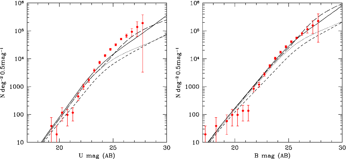
Figure 13: Measured surface densities in the U and B band (red points), plotted with evolution models from Metcalfe et al. (1996) and Metcalfe et al. (2001). The short-dashed lines represent the pure luminosity evolution model, the long-dashed lines the same model with the inclusion of a population of star-forming dwarf galaxies, and the solid lines the same pure luminosity evolution model with a steep faint-end slope of the luminosity function. The latter is in very good agreement with the B-band counts, while the U-band counts are under-predicted by all models.

The models compiled by Metcalfe et al. (1996) and Metcalfe et al. (2001) (normalized to 18 mag using all data available in the bibliography) are plotted against our measurements for the U and B bands in Fig. 13. We plot here three of the models presented in Metcalfe et al. (1996) and Metcalfe et al. (2001). The short-dashed lines represent the pure luminosity evolution model, the long-dashed line the same model with the inclusion of a population of star-forming dwarf galaxies, which is the best-fit model in Metcalfe et al. (1996) and the solid line is the same pure luminosity evolution model with a modification of the faint-end slope of the luminosity functions of late-type spirals ($\alpha=-1.75$ instead of $\alpha=-1.5$), used to fit the multi-colour data of Metcalfe et al. (2001). We find very good agreement with the $\alpha=-1.75$ model in the B-band, although the U-band counts are under-predicted by all models. However, the faint-end slope of the U-band counts does seem to support a steepening of the faint-end slope of the LF. Barro et al. (2009) have shown that the slope of the number count distribution assymptotically reaches $-0.4(\alpha+1)$, where $\alpha$ is the faint-end slope of the luminosty function if parametrized by a Schechter function. Measuring the slopes of the number counts using the five faintest points of each distribution, we calculate the faint-end slopes of the respective luminosity functions: $\alpha_{U}=-1.733\pm 0.018$, $\alpha_{B}=-1.748\pm 0.006$, $\alpha_{V}=-1.507\pm 0.018$. We note that the assumed steep LF faint end slope is in good agreement with the number count distributions of the U and B bands, whereas the V band points to a LF with $\alpha=-1.5$ (see Metcalfe et al., 2001).

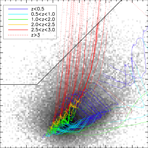
Figure 12: The same plot as Fig. 7, but with with SEDs created with the GISSEL98 code (Bruzual & Charlot, 1993) with different metallicity and extinction properties (see Bolzonella et al., 2000). We use elliptical, irregular and spiral tracks, colour-coded with redshift ranges. The bulk of the distribution is reproduced with spiral and irregular tracks at redshift $0.5<z<2.5$. The $z\gtrsim 3$ region is also marked.

At this point it is useful to have a notion about the type of galaxies that are best represented in our sample and their redshifts. A valuable tool in this direction is the colour distribution; Fig. 7 shows the colour plot of the Lockman Hole sources with tracks of templates of different types of galaxies. We note that the spiral (Sbc-Scd) and irregular tracks lie closer to the bulk of observed colours. The metallicity and extinction properties of a galaxy can have a severe effect in its optical colours. For that reason we reproduce Fig. 7 with a set of SED templates which have varying stellar ages, metallicities and extinctions, calculated with the GISSEL98 code (Bruzual & Charlot, 1993). The results are presented in Fig. 12, where the colour tracks are colour-coded with respect to the redshift. The distribution of sources is well reproduced and we can see that the redshift range most represented is $z=1.5\pm 1$. Moreover, the bulk of the colour distribution is represented by spiral and irregular tracks, while the ellipticals account for colours redder than $B-V=1$.

The galaxy types and redshift probed by our survey are compatible with the “steep faint end slope” model of Metcalfe et al. (2001) and the slopes are also in good agreement. Therefore, there is no need to invoke a dwarf galaxy population to assist the sources which cause the steepening of the faint end slope, in order to reproduce the B-band data. The U-band counts on the other hand are underestimated by the “steep faint end slope” model, although the slope itself agrees. In this case a dwarf galaxy population would assist in incrasing the U-band number counts. It would be however challenging, as such a population is required to affect the U-band leaving the B-band unchanged. The Ly-$\alpha$ line falls into the U wavelength range at a redshift of $z=2$, so a population if highly ionized Ly-$\alpha$ emitters is a good candidate. However, at $z=2.5$ the blue filter would also be affected, which leaves a narrow redshift window for this hypothetical population. An implication of this scenario is a sizeable decrease in the star formation rate between $z=2$ and $z=2.5$. Reddy et al. (2008) find an increase in the star formation rate density between $z\sim 3$ and $z\sim 2$, which is reflected in the UV luminosity density, and more specifically in the number density of faint ($M_{\rm AB}(1700\,\AA)>-21$) UV-emitting galaxies.

A steepening of the faint end slope of the (B-band) luminosity function is already evident since the first computation of its values at redshifts $z>0$ (Lilly et al., 1995). These authors find that the slope increases with redshift (out to $z=1.3$) and that this is an effect caused by galaxies with blue optical colours, while the LF of red galaxies shows minimal change in its fitted parameters. This result is backed up by more recent studies (Gabasch et al., 2004; Ilbert et al., 2005; Arnouts et al., 2005; Willmer et al., 2006; Prescott, Baldry & James, 2009) and the general trend is that the not only blue galaxies’ LFs evolve more with redshift than those of redder colours, their faint end slopes are steeper as well. In cases where the LFs are computed with respect to the galaxy type (Ilbert et al., 2006; Zucca et al., 2006), little (if any) evolution of the faint end slope is found for each galaxy type, while the slope is different for each type, the sttepest beeing in irregulars (Zucca et al., 2006) or blue-bulge galaxies (Ilbert et al., 2006). There is however significant change in the normalization and the value of $M^{\star}$ (the characteristic Schechter luminosity), which is interpreted as an increase in the fraction of irregular and late-type galaxies with redshift. The steep faint-end slope we find in the U and B bands ($\alpha\simeq-1.75$) agrees with the values fitted for irregular galaxies by Zucca et al. (2006) and is even a bit too flat compared to the value assumed by Ilbert et al. (2005) for the blue-bulge population (their $\alpha=-2.0$). Given that in this survey the dominant population, especially at faint magnitudes, is spirals and irregulars at non-local redshifts, we support these steep faint-end slopes. The sources responsible for the steep slopes are activly star forming and are good candidates for the “blue dwarf” population. Driver et al. (1995) assume that this population consists of sources with late-type and irregular morphologies; Ilbert et al. (2006) state that the “blue bulge” population could be a population of actively star-forming galaxies, where the starburst region has bulge-like morphological characteristics, like the “blue spheroid” galaxy sample of Im et al. (2001).

An issue that still needs to be addressed is the flattening of the number counts slope in the V-band. A mechanism that affects the faint-end slope is supernova feedback, which is caused by the heating of the interstellar medium through supernova exposions. Nagashima et al. (2005) have modelled galaxy formation taking this effect into account. Their predictions for the number counts using strong or weak feedback (parametrized by the time-scale in which supernova explosions reheat the cold interstellar gas) differ in the faint slope with minimal impact on the normalization (see Figure 18 in Nagashima et al., 2005). Fig. 14 plots the B and V-band number counts predictions of Nagashima et al. (2005) with our data-points; the solid and dashed lines refer to strong and weak feedback respectively. While both predictions seem to overestimate the observed number counts at faint fluxes, the faint end slope of the weak feedback prediction is in good agreement with the data for the B-band, while the V-band slope is better interpreted with the strong feedback model. A possible explanation is that the V-band probes the same rest frame wavelength at higher redshift. If we assume that star formation is the dominant mechanism producing near-infrared light (where the rest-frame B and V bands are at redshift $z>1.5$) the V-band probes higher redshifts than the B-band. There is evidence that the UV luminosity function has a steeper faint end slope at $z\sim 2$ ($\alpha=-1.88\pm 0.27$, Reddy et al., 2008) than at $z\sim 3$ ($\alpha=-1.60\pm 0.13$, Steidel et al., 1999). In this case, starburst feedback would be stronger at higher redshift, in line with our data. So, enhanced SFR at $z>1.5$ could cause the flattening of the V-band faint slope.

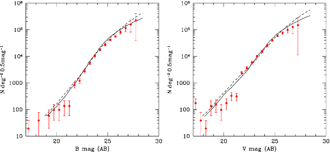
Figure 14: Measured surface densities in the B and V band (red points), plotted with number counts from the simulations of Nagashima et al. (2005). The solid and dashed lines represent the strong and weak supernova feedback cases respectively. The faint end slope of the weak feedback model is in better agreement with the B-band data, while the the strong feedback model is in better agreement with the V-band data.

6.2 Colour selection

To be able to test evolutionary models of galaxies in a greater extent one needs to have information of the redshifts of the various objects found in a “blind” survey. However, even with the largest telescopes available it is practically impossible to have complete samples beyond $R\sim 24$ and use the full capacity of photometric surveys. Moreover, the selection of targets for spectroscopy at such faint limits is hard because their redshift range is so large that it makes it impossible to get meaningful spectra without pre-selecting the targets according to their redshift range. A way to overcome this barrier is to use the photometric redshift technique, where the SED of each source is compared with known SED templates to derive an estimate of the redshift. Although the accuracy of this method is limited so it cannot be used for e.g. spatial clustering studies it can be very useful in deriving luminosities or selecting objects in different redshift ranges. Given the extensive spectral coverage of the Lockman Hole it is possible to calculate photometric redshifts for a large number of galaxies. Details about the Lockman Hole photo-z survey will be given in a subsequent paper.

The drawback of the photometric redshift technique is that it requires the detection of the source in a large number of bands spanning from the near ultraviolet to the infrared. It is however possible to select sources within a redshift range using the “dropout” technique (e.g. Steidel et al., 2003). This technique is used to detect the Lyman break in the spectra of galaxies when it is redshifted between two of the observed bands. In practice the colour-colour diagram is used to select the sources. Based on the colour tracks of Fig. 12, we set the selection limits of sources with $z\gtrsim 3$ to:

$$U-B>0.9$$

$$U-B>B-V+1.2$$

$$B-V<1.3$$

Using these limits, we find 2152 sources with redshift $z\gtrsim 3$ in the whole Lockman Hole region (925 arcmin²), which gives a number density of 8375 deg^-2. Steidel et al. (2003) find 6176 deg^-2 U-dropout $z\sim 3$ sources using different selection bands ($U_{n}-G$ vs. $G-\cal R$). Using the near-infrared coverage of the Lockman Hole we could also select sources according to their B-z-K colours (see Daddi et al., 2004), having $1.4<z<2.5$, or according to their i-z colour, having $1.4<z<2.5$ (see Vanzella et al., 2005). Being able to select sources in distinct redshift ranges provides a valuable tool to further test models of galaxy evolution.

Selecting sources by their colours can also provide samples of different kinds of objects. Compton thick AGN are active galaxies with dense environments ($N_{\rm H}>10^{24}\,{\rm cm}^{-2}$) so that they block even hard X-ray radiation and are not detected even in the deepest X-ray surveys. They would provide valuable information in evolution studies, as they represent a distinctive phase of a galaxies lifetime and they are the “missing link” in population synthesis models of the X-ray background (Gilli, Comastri & Hasinger, 2007). The most promising methods of detecting Compton thick AGN involves comparing the optical and infrared fluxes of sources (Donley et al., 2007; Daddi et al., 2007; Fiore et al., 2008; Georgantopoulos et al., 2008). The multi wavelength coverage of the Lockman Hole in combination with the deep X-ray observations are ideal for this kind of study.

6.3 Follow-up

One important contribution of this study is that it provides a large number of newly detected extragalactic objects to be further observed in follow-up campaigns. A number of sources has already been spectroscopically identified, and they have been selected from the X-ray campaigns with ROSAT (Schmidt et al., 1998; Lehmann et al., 2000, 2001) and XMM-Newton (Mateos et al., 2005). With multi-object spectrographs we are now able to conduct spectroscopy to a large number of optical sources. The LBT is already equipped with a near-infrared multi-slit spectrograph (LUCIFER; Mandel et al., 2007) which will start operation within 2009 and the optical multi-slit spectrograph (MODS; Pogge et al., 2006) is expected to be operational in 2010. The key scientific goals of these instruments is to conduct spectroscopy at cosmologically interesting redshifts. To be able to select targets for these instruments we need a deep optical survey and a colour selection scheme similar to what described in the previous section.

7 Summary and conclusions

In this paper we present the deep imaging campaign of the Lockman Hole using the LBT. The Lockman Hole is an excellent region for deep multi-wavelength observations given the minimal galactic absorption. Here we report details of the U, B, and V-band observation and the data reduction strategy. Our imaging area covers 925 arcmin² in a very well sampled region of the Lockman Hole, with deep X-ray, infrared, and radio coverage. We have reached depths of 26.7, 26.3, and 26.3 mag(AB) in the U, B, and V band respectively, in terms of 50% source detection efficiency, and have extracted a large number of sources ($\sim 85000$) an all three bands.

The number counts distributions are used to test galaxy evolution models and and simulations. We find evidence of steepening of the faint-end slope of the luminosity function in the U and B bands, which can explain the B number count without the need of a dwarf galaxy population. However the U counts are under-predicted with this model and an enhancement of the star formation rate at $z=1.5-2.5$ is needed to explain them. A flatter faint end slope observed in the V-band case could be the result of supernova feedback.

This survey is part of an effort to conduct deep observations of the Lockman Hole in different bands ranging from the infrared to the X-rays. This will help us select different source classes for further study and in addition to planned spectroscopic observations create a large database for extragalactic studies.