Estimating the Gumbel scale parameter for local alignment of random sequences by importance sampling with stopping times

Abstract

The gapped local alignment score of two random sequences follows a Gumbel distribution. If computers could estimate the parameters of the Gumbel distribution within one second, the use of arbitrary alignment scoring schemes could increase the sensitivity of searching biological sequence databases over the web. Accordingly, this article gives a novel equation for the scale parameter of the relevant Gumbel distribution. We speculate that the equation is exact, although present numerical evidence is limited. The equation involves ascending ladder variates in the global alignment of random sequences. In global alignment simulations, the ladder variates yield stopping times specifying random sequence lengths. Because of the random lengths, and because our trial distribution for importance sampling occurs on a different sample space from our target distribution, our study led to a mapping theorem, which led naturally in turn to an efficient dynamic programming algorithm for the importance sampling weights. Numerical studies using several popular alignment scoring schemes then examined the efficiency and accuracy of the resulting simulations.

copyrightownerIn the Public Domain

, and

1 Introduction

Sequence alignment is an indispensable tool in modern molecular biology. As an example, BLAST 1 , 2 , 3 (the Basic Local Alignment Search Tool, http://www.ncbi.nlm.nih.gov/BLAST/), a popular sequence alignment program, receives about $2.89$ submissions per second over the Internet. Currently, BLAST users can choose among only 5 standard alignment scoring systems, because BLAST $p$-values must be pre-computed with simulations that take about 2 days for the required $p$-value accuracies. Moreover, adjustments for unusual amino acid compositions are essential in protein database searches 4 , and in that application, computational speed demands that the corresponding $p$-values be calculated with crude, relatively inaccurate approximations 2 . Accordingly, for more than a decade, much research has been directed at estimating BLAST $p$-values in real time (i.e., in less than 1 sec) 5 , 6 , 7 , 8 , so that BLAST might use arbitrary alignment scoring systems.

Several studies have used importance sampling to estimate the BLAST $p$-value 6 , 8 , 9 . To describe importance sampling briefly, let $\mathbb{E}$ denote the expectation for some “target distribution” $\mathbb{P}$, let $\mathbb{Q}$ be any distribution, and consider the equation

$$\mathbb{E}X:=\int X(\omega)\,d\mathbb{P}(\omega)=\int X(\omega)\frac{d\mathbb{P}(\omega)}{d\mathbb{Q}(\omega)}\,d\mathbb{Q}(\omega).$$ (1)

A computer can draw samples $\omega_{i}$ $(i=1,\ldots,r)$ from the “trial distribution” $\mathbb{Q}$ to estimate the expectation: $\mathbb{E}X\approx r^{-1}\sum_{i=1}^{r}X(\omega_{i})[d\mathbb{P}(\omega_{i})/d\mathbb{Q}(\omega_{i})]$. The name “importance sampling” derives from the fact that the subsets of the sample space where $X$ is large dominate contributions to $\mathbb{E}X$. By focusing sampling on the “important” subsets, judicious choice of the trial distribution $\mathbb{Q}$ can reduce the effort required to estimate $\mathbb{E}X$. In importance sampling, the likelihood ratio $d\mathbb{P}(\omega)/d\mathbb{Q}(\omega)$ is often called the “importance sampling weight” (or simply, the “weight”) of the sample $\omega$.

A Monte Carlo technique called “sequential importance sampling” can substantially increase the statistical efficiency of importance sampling by generating samples from $\mathbb{Q}$ incrementally and exploiting the information gained during the increments to guide further increments. Although sequences might seem an especially natural domain for sequential sampling, most simulation studies for BLAST $p$-values have used sequences of fixed length. In contrast, our study involves sequences of random length.

Here, as in several other importance sampling studies 6 , 8 , 9 , 10 , hidden Markov models generate a trial distribution $\mathbb{Q}$ of random alignments between two sequences, where the sequences have a target distribution $\mathbb{P}$. The other studies gloss over the fact that their trial and target distributions occur on different sample spaces, such as alignments and sequences. The other studies used sequences of fixed lengths, however, where a relatively simple formula for the weight $d\mathbb{P}/d\mathbb{Q}$ pertains. For the sequences of random length in this paper, however, the stopping rules for sequential sampling complicate formulas for $d\mathbb{P}/d\mathbb{Q}$. Accordingly, the Appendix gives a general mapping theorem giving formulas for the weights $d\mathbb{P}/d\mathbb{Q}$ when each sample from $\mathbb{P}$ corresponds to many different samples from $\mathbb{Q}$. (In the present article, e.g., each pair of random sequences corresponds to many possible random alignments.) In addition to the mapping theorem, we also develop several other techniques specifically tailored to speeding the estimation of the BLAST $p$-value.

The organization of this article follows. Section 2 on background and notation is divided into 4 subsections containing: (1) a friendly introduction to sequence alignment and its notation; (2) a brief self-contained description of the algorithm for calculating global alignment scores; (3) a technical summary of previous research on estimating the BLAST $p$-value introducing our importance sampling methods; and (4) a heuristic model for random sequence alignment using Markov additive processes. Section 3 on Methods is also divided into 4 subsections containing: (1) a novel formula for the relevant Gumbel scale parameter $\lambda$; (2) a Markov chain model for simulating sequence alignments (borrowed directly from a previous study 10 , but used here with a stopping time); (3) a dynamic programming algorithm for calculating the importance sampling weights in the presence of a stopping time; and (4) formulas for the simulation errors. Section 4 then gives numerical results for the estimation of $\lambda$ under 5 popular alignment scoring schemes. Finally, Section 5 is our Discussion.

2 Background and notation

2.1 Sequence alignment and its notation

Let $\mathbf{A}=A_{1}A_{2}\cdots$ and $\mathbf{B}=B_{1}B_{2}\cdots$ be two semi-infinite sequences drawn from a finite alphabet $\mathfrak{L}$, for example, $\{\mathrm{A},\mathrm{C},\mathrm{D},\mathrm{E},\mathrm{F},\mathrm{G},\mathrm{H},\mathrm{I},\mathrm{K},\mathrm{L},\mathrm{M},\mathrm{N},\mathrm{P},\mathrm{Q},\mathrm{R},\mathrm{S},\mathrm{T},\mathrm{V},\mathrm{W},\mathrm{Y}\}$ (the amino acid alphabet) or $\{\mathrm{A},\mathrm{C},\mathrm{G},\mathrm{T}\}$ (the nucleotide alphabet). Let $s\dvtx\mathfrak{L}\times\mathfrak{L}\mapsto\mathbb{R}$ denote a “scoring matrix.” In database applications, $s(a,b)$ quantifies the similarity between $a$ and $b$, for example, the so-called “PAM” (point accepted mutation) and “BLOSUM” (block sum) scoring matrices can quantify evolutionary similarity between two amino acids 11 , 12 .

The alignment graph $\Gamma_{\mathbf{A},\mathbf{B}}$ of the sequence-pair $(\mathbf{A},\mathbf{B})$ is a directed, weighted lattice graph in two dimensions, as follows. The vertices $v$ of $\Gamma_{\mathbf{A},\mathbf{B}}$ are nonnegative integer points $(i,j)$. (Below, “$:=$” denotes a definition, e.g., the natural numbers are $\mathbb{N}:=\{1,2,3,\ldots\}$. Throughout the article, $i,j,k,m,n$ and $g$ are integers.) Three sets of directed edges $e$ come out of each vertex $v=(i,j)$: northward, northeastward and eastward (see Figure 1). One northeastward edge goes into $v=(i+1,j+1)$ with weight $s[e]=s(A_{i+1},B_{j+1})$. For each $g>0$, one eastward edge goes into $v=(i+g,j)$ and one northward edge goes into $v=(i,j+g)$; both are assigned the same weight $s[e]=-w_{g}<0$. The deterministic function $w\dvtx\mathbb{N}\mapsto(0,\infty]$ is called the “gap penalty.” (The value $w_{g}=\infty$ is explicitly permitted.) This article focuses on affine gap penalties $w_{g}=\Delta_{0}+\Delta_{1}g$ $(\Delta_{0},\Delta_{1}\geq 0)$, which are typical in BLAST sequence alignments. Together, the scoring matrix $s(a,b)$ and the gap penalty $w_{g}$ constitute the “alignment parameters.”

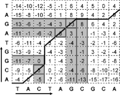
Figure 1: Gapped global alignment scores and the corresponding directed paths for two subsequences $\mathbf{A}[1,10]=\mathsf{TACTAGCGCA}$ and $\mathbf{B}[1,9]=\mathsf{ACGGTAGAT}$, drawn from the nucleotide alphabet $\{\mathsf{A},\mathsf{C},\mathsf{G},\mathsf{T}\}$. Figure 1 uses a nucleotide scoring matrix, where $s(a,b)=5$ if $a=b$ and $-4$ otherwise, and the affine gap penalty $w_{g}=3+2g$. The vertex $(i,j)$ is in the northeast corner of the cell $(i,j)$, with the origin $(0,0)$ at the southwest corner of Figure 1. The cell $(i,j)$ displays the global score $S_{i,j}$, calculated from (3). The optimal global path ending at the point $(10,8)$, for example, consists of $12$ edges, in order: $1$ east of length $1,2$ northeast, $1$ north of length $2,3$ northeast, $1$ east of length $3$, and $1$ northeast. The optimal global score $S_{10,8}=-5+5+5-7+5+5+5-9+5=9$ is the sum of the corresponding edges and represents the path of greatest weight starting at $(0,0)$ and ending at $(10,8)$. The corresponding optimal global alignment of the subsequences $\mathbf{A}[1,10]$ and $\mathbf{B}[1,9]$ is                                             $\mathsf{TAC}\mbox{--}\,\mbox{--}\mathsf{TAGCGCA}$                                             $-\mathsf{ACGGTAG}\mbox{--}\,\mbox{--}\,\mbox{--}\mathsf{A}$.The edge maxima are $M_{1}=-4,M_{2}=0,M_{3}=5,M_{4}=1,M_{5}=3,M_{6}=8,M_{7}=13,M_{8}=9$, $M_{9}=6$. The shading and the double lines indicate squares where a vertex (surrounded by double lines) generated an SALE $\beta(k)$. The SALE scores are $M_{\beta(1)}=\break M_{3}=5,M_{\beta(2)}=M_{6}=8,M_{\beta(3)}=M_{7}=13;$ and the global maximum $M$ for $\mathbf{A}$ and $\mathbf{B}$ is no less than $13$, the largest global score shown.

A (directed) path $\pi=(v_{0},e_{1},v_{1},e_{2},\ldots,e_{k},v_{k})$ in $\Gamma_{\mathbf{A},\mathbf{B}}$ is a finite alternating sequence of vertices and edges that starts and ends with a vertex. For each $i=1,2,\ldots,k$, the directed edge $e_{i}$ comes out of vertex $v_{i-1}$ and goes into vertex $v_{i}$. We say that the path $\pi$ starts at $v_{0}$ and ends at $v_{k}$.

Denote finite subsequences of the sequence $\mathbf{A}$ by $\mathbf{A}[i,m]=A_{i}A_{i+1}\cdots A_{m}$. Every gapped alignment of the subsequences $\mathbf{A}[i,m]$ and $\mathbf{B}[j,n]$ corresponds to exactly one path that starts at $v_{0}=(i-1,j-1)$ and ends at $v_{k}=(m,n)$ (see Figure 1). The alignment’s score is the “path weight” $S_{\pi}:=\sum_{i=1}^{k}s[e_{i}]$.

Define the “global score” $S_{i,j}:=\max_{\pi}S_{\pi}$, where the maximum is taken over all paths $\pi$ starting at $v_{0}=(0,0)$ and ending at $v_{k}=(i,j)$. The paths $\pi$ starting at $v_{0}$, ending at $v_{k}$, and having weight $S_{\pi}=S_{i,j}$ are “optimal global paths” and correspond to “optimal global alignments” between $\mathbf{A}[1,i]$ and $\mathbf{B}[1,j]$. Define the “edge maximum” $M_{n}:=\max\{\max_{0\leq i\leq n}S_{i,n},\max_{0\leq j\leq n}S_{n,j}\}$, and the “global maximum” $M:=\sup_{n\geq 0}M_{n}$. (The single subscript in $M_{n}$ indicates that the variate corresponds to a square $[0,n]\times[0,n]$, rather than a general rectangle $[0,m]\times[0,n]$.) Define the “strict ascending ladder epochs” (SALEs) in the sequence $(M_{n})$: let $\beta(0):=0$ and $\beta(k+1):=\min\{n>\beta(k)\dvtx M_{n}>M_{\beta(k)}\}$, where $\min\varnothing:=\infty$. We call $M_{\beta(k)}$ the “$k$th SALE score.”

Define also the “local score” $\tilde{S}_{i,j}:=\max_{\pi}S_{\pi}$, where the maximum is taken over all paths $\pi$ ending at $v_{k}=(i,j)$, regardless of their starting point. Define the “local maximum” $\tilde{M}_{m,n}:=\max_{0\leq i\leq m,0\leq j\leq n}\tilde{S}_{i,j}$. The paths $\pi$ ending at $v_{k}=(i,j)$ with local score $S_{\pi}=\tilde{S}_{i,j}=\tilde{M}_{m,n}$ are “optimal local paths” corresponding to the “optimal local alignments” between subsequences of $\mathbf{A}[1,m]$ and $\mathbf{B}[1,n]$.

Now, the following “independent letters” model introduces randomness. Choose each letter in the sequence $\mathbf{A}$ and $\mathbf{B}$ randomly and independently from the alphabet $\mathfrak{L}$ according to fixed probability distributions $\{p_{a}\dvtx a\in\mathfrak{L}\}$ and $\{p^{\prime}_{b}\dvtx b\in\mathfrak{L}\}$. (Although this article permits the distributions $\{p_{a}\}$ and $\{p^{\prime}_{b}\}$ to be different, in applications they are usually the same.) Throughout the paper, the probability and expectation for the independent letters model are denoted by $\mathbb{P}$ and $\mathbb{E}$.

Let $\Gamma=\Gamma_{\mathbf{A},\mathbf{B}}$ denote the random alignment graph of the sequence-pair $(\mathbf{A},\mathbf{B})$. In the appropriate limit, if the alignment parameters are in the so-called “logarithmic phase” 13 , 14 (i.e., if the optimal global alignment score of long random sequences has a negative score), the random local maximum $\tilde{M}_{m,n}$ follows an approximate Gumbel extreme value distribution with “scale parameter” $\lambda$ and “pre-factor” $K$ 15 , 16 ,

$$\mathbb{P}(\tilde{M}_{m,n}>y)\approx 1-\exp[-Kmn\exp(-\lambda y)].$$ (2)

2.2 The dynamic programming algorithm for global sequence alignment

For affine gaps $w_{g}=\Delta_{0}+\Delta_{1}g$, the global score $S_{i,j}$ is calculated with the recursion

$$S_{i,j}=\max\{S_{i-1,j-1},I_{i-1,j-1},D_{i-1,j-1}\}+s(A_{i},B_{j}),$$ (3)

where

$$I_{i,j}=\max\{S_{i,j-1}-\Delta_{0}-\Delta_{1},I_{i,j-1}-\Delta_{1},D_{i,j-1}-\Delta_{0}-\Delta_{1}\},$$

$D_{i,j}=\max\{S_{i-1,j}-\Delta_{0}-\Delta_{1},D_{i-1,j}-\Delta_{1}\}$ and boundary conditions $S_{0,0}=0,I_{0,0}=D_{0,0}=-\infty,D_{g,0}=I_{0,g}=-\Delta_{0}-\Delta_{1}g,S_{g,0}=S_{0,g}=I_{g,0}=D_{0,g}=-\infty$ for $g>0$ 17 . The three array names, $S,I$, and $D$, are mnemonics for “substitution,” “insertion” and “deletion.” If “$\Delta$” denotes a gap character, the corresponding alignment letter-pairs $(a,b),(\Delta,b)$ and $(a,\Delta)$ correspond to the operations for editing sequence $\mathbf{A}$ into sequence $\mathbf{B}$ 18 .

2.3 Previous methods for estimating the BLAST $p$-value

If $w_{g}\equiv\infty$ identically, so northward and eastward (gap) edges are disallowed in an optimal alignment path, a rigorous proof of (2) yields analytic formulas for the Gumbel parameters $\lambda$ and $K$ 14 . For gapped local alignment, rigorous results are sparse, although some approximate analytical studies are extant 7 , 19 , 20 , 21 . The prevailing approach therefore estimates $\lambda$ and $K$ from simulations 22 , 23 . Because $\lambda$ is an exponential rate, it dominates $K$’s contribution to the BLAST $p$-value. Most studies therefore (including the present one) have focused on $\lambda$. (Note, however, some recent progress on the real-time estimation of $K$ 6 .) Typically, current applications require a 1–4% relative error in $\lambda$; 10–20%, in $K$ 23 . The characteristics of the relevant sequence database determine the actual accuracies required, however, making approximations with controlled error and of arbitrary accuracy extremely desirable in practice.

Storey and Siegmund 7 approximate $\lambda$ (with neither controlled errors nor arbitrary accuracy) as

$$\tilde{\lambda}\approx\lambda^{*}-2(\mu^{*})^{-1}\Lambda e^{-\lambda^{*}\Delta_{0}}/(e^{\lambda^{*}\Delta_{1}}-1),$$ (4)

where $\sum_{(a,b)}p_{a}p^{\prime}_{b}\exp[\lambda^{*}s(a,b)]=1$ [so $\lambda^{*}$ is the so-called “ungapped lambda,” for $\Delta(g)\equiv\infty$] and $\mu^{*}:=\sum_{(a,b)}s(a,b)p_{a}p^{\prime}_{b}\exp[\lambda^{*}s(a,b)]$. In (4), $\Lambda$ is an upper bound for an infinite sequence of constants defined in terms of gap lengths in a random alignment.

Many other studies have used local alignment simulations to estimate BLAST $p$-values, for example, Chan 9 used importance sampling and a mixture distribution. Some rigorous results 24 are also extant for the so-called “island method” 22 , 25 , which yields maximum likelihood estimates of $\lambda$ and $K$ from a Poisson process associated with local alignments exceeding a threshold score 23 , 26 .

Large deviations arguments 13 , 27 support the common belief that global alignment can estimate $\lambda$ for local alignment through the equation $\lambda=\break-\lim_{y\to\infty}y^{-1}\ln\mathbb{P}\{M\geq y\}$. For a fixed error, global alignment typically requires less computational effort than local alignment. For example, one early study 10 used importance sampling based on trial distributions $\mathbb{Q}$ from a hidden Markov model.

The study demonstrated that the global alignment equation $\mathbb{E}[\exp(\lambda S_{n,n})]=1$ estimated $\lambda$ with only $O(n^{-1})$ error 8 . (Recall that “$\mathbb{E}$” denotes theexpectation corresponding to the random letters model.) The equation$\mathbb{E}[\exp(\lambda M_{m})]=\mathbb{E}[\exp(\lambda M_{n})]$ $(m\neq n)$, suggested by heuristic modeling with Markov additive processes (MAPs) 28 , 29 , improved the error substantially, to $O(\varepsilon^{n})$ 5 .

The next subsection shows how the MAP heuristic can improve the efficiency of importance sampling even further, with its renewal structure. The next subsection gives the relevant parts of the MAP heuristic.

2.4 The Markov additive process heuristic

The rigorous theory of MAPs appears elsewhere 28 , 29 . Because the MAP heuristics given below parallel a previous publication 5 , we present only informal essentials.

Consider a finite Markov-chain state-space $\mathfrak{J}$, containing $\#\mathfrak{J}$ elements. Without loss of generality, $\mathfrak{J}=\{1,\ldots,\#\mathfrak{J}\}$. Until further notice, all vectors are row vectors of dimension $\#\mathfrak{J}$; all matrices, of dimension $(\#\mathfrak{J})\times(\#\mathfrak{J})$. A MAP can be defined in terms of a time-homogenous Markov chain (MC) $(J_{n}\in\mathfrak{J}\dvtx n=0,1,\ldots)$ and a $(\#\mathfrak{J})\times(\#\mathfrak{J})$ matrix of real random variates $\|Z_{i,j}\|$. Let the MC have transition matrix $\mathbf{P}=\|p_{i,j}\|$, so $p_{i,j}=\mathbb{P}(J_{n}=j|J_{n-1}=i)$. Let the stationary distribution of the MC be $\bolds{\pi}$, assumed strictly positive and satisfying both $\bolds{\pi}\mathbf{P}=\bolds{\pi}$ and $\bolds{\pi}\mathbf{1}^{t}=1$, where $\mathbf{1}^{t}$ denotes the $(\#\mathfrak{J})\times 1$ column vector whose elements are all $1$.

As usual, let $\mathbb{P}_{\bolds{\gamma}}$ and $\mathbb{E}_{\bolds{\gamma}}$ be the probability measure and expectation corresponding to an initial state $J_{0}$ with distribution $\bolds{\gamma}$; $\mathbb{P}_{i}$ and $\mathbb{E}_{i}$, to an initial state $J_{0}=i$; and $\mathbb{P}_{\bolds{\pi}}$ and $\mathbb{E}_{\bolds{\pi}}$, to an initial state in the equilibrium distribution $\bolds{\pi}$.

Run the MC $(J_{n})$, and take its succession of states as given. Consider the following sequence $(Y_{n}\in\mathbb{R}\dvtx n=0,1,\ldots)$ of random variates. Define $Y_{0}:=0$. For $n=1,2,\ldots,$ let the $(Y_{n})$ be conditionally independent, with distributions determined by the transition $J_{n-1}\to J_{n}$ of the Markov chain as follows. If $J_{n-1}=i$ and $J_{n}=j$, the value of $Y_{n}$ is chosen randomly from the distribution of $Z_{i,j}$. (Thus, if $J_{m-1}=J_{n-1}=i$ and $J_{m}=J_{n}=j,Y_{m}$ and $Y_{n}$ share the distribution of $Z_{i,j}$, although independence permits randomness to give them different values.)

The random variates of central interest are the sums $T_{n}=\sum_{m=0}^{n}Y_{m}$ $(n=0,1,\ldots)$ and the maximum $M:=\max_{n\geq 0}T_{n}$. To exclude trivial distributions for $M$ (i.e., $M=0$ a.s. and $M=\infty$ a.s.), make two assumptions: (1) $\mathbb{E}_{\bolds{\pi}}Y_{1}<0$; and (2) there is some $m$ and state $i$ such that

$$\mathbb{P}_{i}\bigl{\{}\min\{T_{k}\dvtx k=1,\ldots,m\}>0;J_{m}=i,J_{j}\neq i\mbox{ for }j=1,\ldots,m-1\bigr{\}}>0.$$ (5)

Consider the sequence $(T_{n})$, its SALEs $\beta(0):=0$ and $\beta(k+1):=\min\{n>\beta(k)\dvtx T_{n}>T_{\beta(k)}\}$, and its SALE scores $T_{\beta(k)}$. For brevity, let $\beta:=\beta(1)$. Note that $M=T_{\beta(k)}$ for some $k\in\{0,1,\ldots\}$. In a MAP, $(J_{\beta(k)},T_{\beta(k)})$ forms a defective Markov renewal process.

Now, define the matrix $\mathbf{L}_{\theta}:=\|\mathbb{E}_{i}[\exp(\theta T_{\beta})$; $J_{\beta}=j,\beta<\infty]\|$. The Perron–Frobenius theorem 29 , page 25, shows that $\mathbf{L}_{\theta}$ has a strictly dominant eigenvalue $\rho(\theta)>0$ [i.e., $\rho(\theta$) is the unique eigenvalue of greatest absolute value]. Moreover, $\rho(\theta)$ is a convex function 30 , and because $\mathbf{L}_{0}$ is substochastic, $\rho(0)<1$. The two assumptions above (5) ensure that $M:=\max_{n\geq 0}T_{n}$ has a nontrivial distribution and that $\rho(\lambda)=1$ for some unique $\lambda>0$.

The notation intentionally suggests a heuristic analogy between MAPs and global alignment. Identify the Markov chain states $J_{n}$ in the MAP with the rectangle $[0,n]\times[0,n]$ of $\Gamma_{\mathbf{A},\mathbf{B}}$, and identify the sum $T_{n}$ in the MAP with the edge maximum $M_{n}$ in global alignment. In the following, therefore, the identification leads to $M_{n}$ replacing $T_{n}$ in the MAP formulas. In particular, the MAP heuristic identifies the Gumbel scale parameter in (2) with the root $\lambda>0$ of the equation $\rho(\lambda)=1$. Although the heuristic analogy between MAPs and global alignment is in no way precise or rigorous, it has produced useful results 5 .

The details of why the MAP heuristic works so well are presently obscure, although some additional motivation appears in an heuristic calculation related to $\lambda$ 31 . The calculation takes the limit of nested successively wider semi-infinite strips, each strip having constant width and propagating itself northeastward in the alignment graph $\Gamma_{\mathbf{A},\mathbf{B}}$. The successive northeast boundaries of the propagation are states in an ergodic MC. MAPs therefore might rigorously justify the heuristic calculation.

3 Methods

3.1 A novel equation for $\lambda$

From the definition of $\mathbf{L}_{\theta}$ in a MAP, if the Markov chain $\{J_{n}\}$ starts in a state $J_{0}$ with distribution $\bolds{\gamma}$ (with $M_{n}$ replacing $T_{n}$ in the MAP formulas), matrix algebra applied to the concatenation of SALEs in a MAP yields

$$\mathbb{E}_{\bolds{\gamma}}\bigl{[}\exp\bigl{(}\theta M_{\beta(k)}\bigr{)};\beta(k)<\infty\bigr{]}=\bolds{\gamma}(\mathbf{L}_{\theta})^{k}\mathbf{1}^{t}.$$ (6)

For a MAP, equation (6) is exact; but for global alignment, it has no literal meaning. Equation (6) has some consequences for the limit $k\to\infty$, and we speculate that the consequences hold, even for global alignment. [Note: although the sequence $(\beta(k))$ is a.s. finite, the limits $k\to\infty$ below involve no contradiction or approximation, because they are not a.s. limits.]

Define $K_{k}(\theta):=\ln\{\mathbb{E}_{\bolds{\gamma}}[\exp(\theta M_{\beta(k)});\beta(k)<\infty]\}$. In (6), a spectral (eigenvalue) decomposition of the matrix $\mathbf{L}_{\theta}$ 32 shows that

$$K_{k}(\theta)=k\ln\{\rho(\theta)\}+c_{0}+O(\varepsilon^{k}),$$ (7)

where $0\leq\varepsilon<1$ is determined by the magnitude of the subdominant eigenvalue of $\mathbf{L}_{\theta}$, and $c_{0}$ is a constant independent of $\theta$ and $k$.

For $k^{\prime}-k>0$ fixed, we can accelerate the convergence in (7) as $k\to\infty$ by differencing

$$K_{k^{\prime}}(\theta)-K_{k}(\theta)=(k^{\prime}-k)\ln\{\rho(\theta)\}+O(\varepsilon^{k}).$$ (8)

Let $\lambda_{k^{\prime},k}$ denote the root of (8) after dropping the error term $O(\varepsilon^{k})$. Because $\rho(\lambda)=1$, Taylor approximation around $\lambda$ yields $\ln\{\rho(\lambda_{k^{\prime},k})\}\approx\rho^{\prime}(\lambda)(\lambda_{k^{\prime},k}-\lambda)$, so (8) becomes

$$(k^{\prime}-k)\rho^{\prime}(\lambda)(\lambda_{k^{\prime},k}-\lambda)=O(\varepsilon^{k}),$$ (9)

that is, with $k^{\prime}-k$ fixed, $\lambda_{k^{\prime},k}$ converges geometrically to $\lambda$ as the SALE index $k\to\infty$.

The initial state $\bolds{\gamma}$ of global alignment has a deterministic distribution, namely the origin $(0,0)$. Equation (8) for $\theta=\lambda$ therefore becomes

$$\mathbb{E}\bigl{[}\exp\bigl{(}\lambda M_{\beta(k^{\prime})}\bigr{)};\beta(k^{\prime})<\infty\bigr{]}=\mathbb{E}\bigl{[}\exp\bigl{(}\lambda M_{\beta(k)}\bigr{)};\beta(k)<\infty\bigr{]}$$ (10)

after dropping the geometric error $O(\varepsilon^{k})$. Let $\hat{\lambda}_{k^{\prime},k}$ be the root of (10).

3.2 The trial distribution for importance sampling

In (10), crude Monte Carlo simulation generating random sequence-pairs with the identical letters model $\mathbb{P}$ is inefficient for the following reason. When practical alignment scoring systems are used, $\mathbb{P}\{\beta(k)<\infty\}<1$ for $k\geq 1$. For, example, the BLAST defaults (scoring matrix BLOSUM62, gap penalty $w_{g}=11+g$, and Robinson–Robinson letter frequencies), $\mathbb{P}\{\beta(4)<\infty\}\approx 0.047$, so only about 1 in 20 crude Monte Carlo simulations generate a fourth ladder point. Empirically in our importance sampling, however, Gumbel parameter estimation seemed most efficient when the stopping time corresponded to $\beta(4)$ (see below).

Importance sampling requires a trial distribution to determine $\hat{\lambda}_{k^{\prime},k}$ from (10). By editing one sequence into another, a Markov chain model borrowed directly from a previous study 10 generates random sequence alignments, as follows.

Consider a Markov state space consisting of the set of alignment letter-pairs $\bar{\mathfrak{L}}^{2}$, where $\bar{\mathfrak{L}}:=\mathfrak{L}\cup\{\Delta\}$, “$\Delta$” being a character representing gaps. The ordered pair $(\Delta,\Delta)$ has probability 0, so a succession of Markov states corresponds to a global sequence alignment (see Figure 1), that is, to a path in the alignment graph $\Gamma_{\mathbf{A},\mathbf{B}}$. Ordered pairs other than $(\Delta,\Delta)$ fall into three sets, corresponding to edit operations following (3): $S:=\mathfrak{L}\times\mathfrak{L}$ [substitution, a bioinformatics term implicitly including identical letter-pairs $(a,a)$], $I:=\{\Delta\}\times\mathfrak{L}$ (insertion); and $D:=\mathfrak{L}\times\{\Delta\}$ (deletion). The sets $S,I$ and $D$ form “atoms” of the MC 33 , page 203, as follows. (By definition, each atom of a MC is a set of all states with identical outgoing transition probabilities.)

From the set $S$, the transition probability to $(a,b)$ is $t_{S,S}q_{a,b}$; to $(\Delta,b),t_{S,I}p^{\prime}_{b}$; and to $(a,\Delta),t_{S,D}p_{a}$. From the set $I$, the transition probability to $(a,b)$ is $t_{I,S}q_{a,b}$; to $(\Delta,b),t_{I,I}p^{\prime}_{b}$; and to $(a,\Delta),t_{I,D}p_{a}$. From the set $D$, the transition probability to $(a,b)$ is $t_{D,S}q_{a,b}$; to $(\Delta,b),t_{D,I}p^{\prime}_{b}$; and to $(a,\Delta),t_{D,D}p_{a}$. Transition probabilities sum to 1, so the following restrictions apply: $\sum_{a,b\in\mathfrak{L}}q_{a,b}=1,\sum_{b\in\mathfrak{L}}p^{\prime}_{b}=1,\sum_{a\in\mathfrak{L}}p_{a}=1,t_{S,S}+t_{S,I}+t_{S,D}=1$ (transit from the substitution atom), $t_{D,D}+t_{D,S}+t_{D,I}=1$ (transit from the deletion atom) and $t_{I,I}+t_{I,S}+t_{I,D}=1$ (transit from the insertion atom). Usually in practice, the term $t_{I,D}=0$, to disallow insertions following a deletion. Our formulas retain the term, to exploit the resulting symmetry later.

In the terminology of hidden Markov models, $S,I,D$ are hidden Markov states. $t_{i,j}$ for $i,j\in\{S,I,D\}$ are transition probabilities and $q_{a,b},p^{\prime}_{b},p_{a}$ for $a,b\in\mathfrak{L}$ are emission probabilities from the state $S,I,D$, respectively.

As described elsewhere 10 , numerical values for the Markov probabilities can be determined from the scores $s(a,b)$ and the gap penalty $w_{g}$. Note that the values are selected for statistical efficiency, although many other values also yield unbiased estimates for $\lambda$ in the appropriate limit.

3.3 Importance sampling weights and stopping times

To establish notation, and to make connections to the Appendix and its mapping theorem, note that the MC above can be supported on a probability space $(\Omega,\mathsf{F},\mathbb{Q})$, where each $\omega=(\pi,\mathbf{A},\mathbf{B})\in\Omega$ is an ordered triple. Here, $\pi$ is an infinite path starting at the origin in the alignment graph $\Gamma_{\mathbf{A},\mathbf{B}};\mathsf{F}$ is the set generated by cylinder sets in $\Omega$ (here, cylinder sets essentially consist of some finite path and the corresponding pair of subsequences); and $\mathbb{Q}$ is the MC probability distribution described above, started at the atom $S$, with expectation operator $\mathbb{E}_{\mathbb{Q}}$.

Let $N$ be any stopping time for the sequence $(M_{n}\dvtx n=0,1,\ldots)$ of edge maxima for $\Gamma_{\mathbf{A},\mathbf{B}}$ (i.e., the sequence $\{M_{0},\ldots,M_{n}\}$ determines whether $N\leq n$ or not). Because $M_{n}$ is determined by $(\mathbf{A}[1,n],\mathbf{B}[1,n]),N$ is also a stopping time for the sequence $\{(\mathbf{A}[1,n],\mathbf{B}[1,n])\dvtx n=0,1,\ldots\}$. The stopping time of main interest here is $N=\beta(k)$, the $k$th ladder index of $(M_{n})$, where $k\geq 1$ is arbitrary. (As further motivation for the mapping theorem in the Appendix, other stopping times of possible interest include, for example, $N=n$, a fixed epoch 8 , and $N=\beta(K_{y})$, where $\beta(K_{y})=\inf\{n\dvtx M_{n}\geq y\}$ is the index of first ladder-score outside the interval $(0,y).)$

To use the mapping theorem, introduce the probability space $(\Omega^{\prime\prime},\mathsf{F}^{\prime\prime},\mathbb{P})$, where each $\omega^{\prime\prime}=(\mathbf{A},\mathbf{B})\in\Omega^{\prime\prime}$ is an ordered pair. Here, $\mathbf{A}$ and $\mathbf{B}$ are sequences, $\mathsf{F}^{\prime\prime}$ is the set generated by all cylinder sets in $\Omega^{\prime\prime}$ (i.e., sets corresponding to pairs of finite subsequences) and $\mathbb{P}(A^{\prime\prime})=\prod_{k=1}^{i}p_{A_{k}}\prod_{k=1}^{j}p^{\prime}_{B_{k}}$, if the cylinder set $A^{\prime\prime}$ corresponds to the subsequence pair $(\mathbf{A}[1,i],\mathbf{B}[1,j])$. Given $N$, the theory of stopping times 29 , page 414, can be used to construct a discrete probability space $(\Omega^{\prime},\mathsf{F}^{\prime},\mathbb{P})$, where each event $\omega^{\prime}\in\Omega^{\prime}$ is a finite-sequence pair $\omega^{\prime}=(\mathbf{A}[1,N],\mathbf{B}[1,N]),\mathsf{F}^{\prime}$ is the set of all subsets of $\Omega^{\prime}$ and $\mathbb{P}(\omega^{\prime})=\prod_{k=1}^{N(\omega^{\prime})}p_{A_{k}}\prod_{k=1}^{N(\omega^{\prime})}p^{\prime}_{B_{k}}$.

Let $\mathsf{I}_{m,n}:=\{(i,j)\dvtx i=m,j\geq n\}$ and $\mathsf{D}_{m,n}:=\{(i,j)\dvtx i\geq m,j=n\}$. Define the function $f\dvtx\omega\mapsto\omega^{\prime}$, where $\omega=(\pi,\mathbf{A},\mathbf{B})$ and $\omega^{\prime}=(\omega^{\prime}_{\mathbf{A}},\omega^{\prime}_{\mathbf{B}}):=(\mathbf{A}[1,N],\break\mathbf{B}[1,N])$. Then, $\omega\in f^{-1}(\omega^{\prime})$, if and only if the path $\pi$ hits the set $\mathsf{I}_{N,N}\cup\mathsf{D}_{N,N}$ at $(i,j)$, so that $\mathbf{A}[1,N]=\omega^{\prime}_{\mathbf{A}}$ and $\mathbf{B}[1,N]=\omega^{\prime}_{\mathbf{B}}$ (see Figure 2).

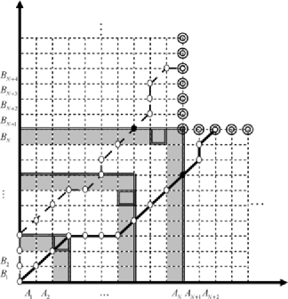
Figure 2: Two examples of alignment path $\pi$ generated by a Markov chain. As in Figure 1, the shading and the double lines indicate squares where a vertex (surrounded by double lines) generated an SALE. The SALEs determine the stopping time $N=\beta(3)$. In Figure 2, the first SALE is determined by the score at the vertex $(3,3);$ the second SALE, the vertex $(7,6);$ the third SALE, the vertex $(9,10)$. Therefore, $N=\beta(3)=10$. The vertical ray $\mathsf{I}_{N,N}$ and the horizontal ray $\mathsf{D}_{N,N}$ are indicated by double circles. The lower path $\pi$ (solid line) ends at $(N+2,N)$ with a final transition to $S$; the upper path $\pi$ (long-dashed line), at $(N,N+4)$ with a final transition to $D$. The closed vertices indicate intersection with the square corresponding to $\omega^{\prime}=(\omega^{\prime}_{\mathbf{A}},\omega^{\prime}_{\mathbf{B}})=(\mathbf{A}[1,N],\mathbf{B}[1,N])$.

Empirically, our simulations satisfied $\mathbb{Q}\{\beta(k)<\infty\}=1$, and we speculate that our application therefore satisfies the hypothesis $\mathbb{Q}H=1$ of the Appendix. According to the Appendix, the reciprocal importance sampling weight $1/W(\omega)=\sum_{\omega_{0}\in f^{-1}\{f(\omega)\}}\mathbb{Q}(\omega_{0})/\mathbb{P}f(\omega)$ depends on the sum over all possible Markov chain realizations $\omega_{0}\in f^{-1}(\omega^{\prime})$. Dynamic programming computes the sum efficiently, as follows.

Let the “transition” $T$ represent any element of $\{S,I,D\}$ [substitution $(a_{i},b_{j})$, insertion $(\Delta,b_{j})$, or deletion $(a_{i},\Delta)$]. Fix any particular pair $(\mathbf{A},\mathbf{B})$ of infinite sequences, which fixes $N=\beta(k)$. To set up a recursion for dynamic programming, consider the following set of events $\mathsf{E}_{i,j}^{T}$, defined for $T\in\{S,I,D\}$ and $\min\{i,j\}\leq N$, and illustrated in Figure 2. Let $\mathsf{E}_{i,j}^{T}$ be the event consisting of all $\omega$ yielding a path $\pi$ whose final transition is $T$ and which corresponds to the subsequences: (1) $\mathbf{A}[1,i]$ and $\mathbf{B}[1,j]$ for $0\leq i,j\leq N$; (2) $\mathbf{A}[1,i]$ and $\mathbf{B}[1,N]$ for $0\leq N=j\leq i$; and (3) $\mathbf{A}[1,N]$ and $\mathbf{B}[1,j]$ for $0\leq N=i\leq j$. Define $Q_{i,j}^{T}:=\mathbb{Q}(\mathsf{E}_{i,j}^{T})$ and $Q_{i,j}:=Q_{i,j}^{S}+Q_{i,j}^{I}+Q_{i,j}^{D}$. (Note: in the following, $T\in\{S,I,D\}$ is always a superscript, never an exponent.)

For brevity, let $\tilde{q}_{i,j}=q_{A_{i},B_{j}}$ for $0\leq i,j\leq N;\tilde{q}_{i,j}=\sum_{(a\in\mathfrak{L})}q_{a,B_{j}}$ for $0\leq j\leq N<i;\tilde{q}_{i,j}=\sum_{(b\in\mathfrak{L})}q_{A_{i},b}$ for $0\leq i\leq N<j$; and $\tilde{q}_{i,j}=1$ otherwise. Let $\tilde{p}^{\prime}_{j}=p^{\prime}_{B_{j}}$ for $0\leq j\leq N$; and $1$ otherwise. Finally, Let $\tilde{p}_{i}=p_{A_{i}}$ for $0\leq i\leq N$; and $1$ otherwise. Because every path into the vertex $(i,j)$ comes from one of three vertices, each corresponding to a different transition $T\in\{S,I,D\}$,

$$Q_{i,j}^{S} = \tilde{q}_{i,j}(t_{S,S}Q_{i-1,j-1}^{S}+t_{I,S}Q_{i-1,j-1}^{I}+t_{D,S}Q_{i-1,j-1}^{D}),$$

$$Q_{i,j}^{I} = \tilde{p}^{\prime}_{j}(t_{S,I}Q_{i,j-1}^{S}+t_{I,I}Q_{i,j-1}^{I}+t_{D,I}Q_{i,j-1}^{D}),$$ (11)

$$Q_{i,j}^{D} = \tilde{p}_{i}(t_{S,D}Q_{i-1,j}^{S}+t_{I,D}Q_{i-1,j}^{I}+t_{D,D}Q_{i-1,j}^{D})$$

with boundary conditions $Q_{0,0}^{S}=1,Q_{0,0}^{I}=Q_{0,0}^{D}=0,Q_{g,0}^{S}=Q_{0,g}^{S}=Q_{g,0}^{I}=Q_{0,g}^{D}=0,Q_{0,g}^{I}=p^{\prime}_{B_{1}}\cdots p^{\prime}_{B_{g}}t_{S,I}(t_{I,I})^{g-1}$ and $Q_{g,0}^{D}=p_{A_{1}}\cdots p_{A_{g}}t_{S,D}\times\break(t_{D,D})^{g-1}$ $(g>0)$.

Recall that $\omega=(\pi,\mathbf{A},\mathbf{B})\in f^{-1}(\omega^{\prime})$, if and only if the path $\pi$ hits the set $\mathsf{I}_{N,N}\cup\mathsf{D}_{N,N}$ at $(i,j)$, so that $\mathbf{A}[1,N]=\omega^{\prime}_{\mathbf{A}}$ and $\mathbf{B}[1,N]=\omega^{\prime}_{\mathbf{B}}$. Thus,

$$\qquad\sum_{\omega\in f^{-1}(\omega^{\prime})}\mathbb{Q}(\omega)=-Q_{N,N}^{S}+\sum_{j=N}^{\infty}(Q_{N,j}^{S}+Q_{N,j}^{D})+\sum_{i=N}^{\infty}(Q_{i,N}^{S}+Q_{i,N}^{I}).$$ (12)

To turn (3.3) into a recursion for importance sampling weights, define $P_{i}:=p_{A_{1}}\cdots p_{A_{\min\{i,N\}}}=\tilde{p}_{1}\cdots\tilde{p}_{i}$ and $P^{\prime}_{j}:=p^{\prime}_{B_{1}}\cdots p^{\prime}_{B_{\min\{j,N\}}}=\tilde{p}^{\prime}_{1}\cdots\tilde{p}^{\prime}_{j}$, and let $W_{i,j}^{T}:=Q_{i,j}^{T}/(P_{i}P^{\prime}_{j})$ $(T\in\{S,I,D\})$. Let $r_{i,j}=\tilde{q}_{i,j}/(\tilde{p}_{i}\tilde{p}^{\prime}_{j})$. For future reference, define $r_{\bullet,j}:=r_{i,j}$ for $0\leq j\leq N<i$ and $r_{i,\bullet}:=r_{i,j}$ for $0\leq i\leq N<j$. Note that $r_{\bullet,j}$ is independent of $i$, and $r_{i,\bullet}$ is independent of $j$. Equation (3.3) yields

$$W_{i,j}^{S} = r_{i,j}(t_{S,S}W_{i-1,j-1}^{S}+t_{I,S}W_{i-1,j-1}^{I}+t_{D,S}W_{i-1,j-1}^{D}),$$

$$W_{i,j}^{I} = t_{S,I}W_{i,j-1}^{S}+t_{I,I}W_{i,j-1}^{I}+t_{D,I}W_{i,j-1}^{D},$$ (13)

$$W_{i,j}^{D} = t_{S,D}W_{i-1,j}^{S}+t_{I,D}W_{i-1,j}^{I}+t_{D,D}W_{i-1,j}^{D}$$

with boundary conditions $W_{0,0}^{S}=1,W_{0,0}^{I}=W_{0,0}^{D}=0,W_{g,0}^{S}=W_{0,g}^{S}=W_{0,g}^{I}=W_{g,0}^{D}=0,W_{0,g}^{I}=t_{S,I}(t_{I,I})^{g-1}$ and $W_{g,0}^{D}=t_{S,D}(t_{D,D})^{g-1}$ $(g>0)$. Because of (12), the importance sampling weight $W:=W(\omega)$ satisfies

$$\frac{1}{W} = \frac{\sum_{\omega_{0}\in f^{-1}\{f(\omega)\}}\mathbb{Q}(\omega_{0})}{\mathbb{P}f(\omega)}$$

$$= -W_{N,N}^{S}+\sum_{j=N}^{\infty}(W_{N,j}^{S}+W_{N,j}^{D})+\sum_{i=N}^{\infty}(W_{i,N}^{S}+W_{i,N}^{I}).$$

Because $r_{i,j}=r_{\bullet,j}$ $(0\leq j\leq N<i)$ and $r_{i,j}=r_{i,\bullet}$ $(0\leq i\leq N<j)$, only a finite number of recursions are needed to compute the infinite sums in (3.3), as follows. For $T\in\{S,I,D\}$, define $\tilde{U}_{i}^{T}:=U_{i,N}^{T}$, where $U_{m,n}^{T}:=\sum_{j=n}^{\infty}W_{m,j}^{T}$. Likewise, define $\tilde{V}_{j}^{T}:=V_{N,j}^{T}$, where $V_{m,n}^{T}:=\sum_{i=m}^{\infty}W_{i,n}^{T}$. Equation (3.3) becomes

$$\frac{1}{W}=-W_{N,N}^{S}+\tilde{U}_{N}^{S}+\tilde{U}_{N}^{D}+\tilde{V}_{N}^{S}+\tilde{V}_{N}^{I}.$$ (15)

Note that $U_{i,j-1}^{T}-U_{i,j}^{T}=W_{i,j-1}^{T}$. To determine $\tilde{U}_{N}^{T}$, summation of (3.3) for $0\leq i\leq N<j$ yields

$$\qquad U_{i,j}^{S} = r_{i,\bullet}(t_{S,S}U_{i-1,j-1}^{S}+t_{I,S}U_{i-1,j-1}^{I}+t_{D,S}U_{i-1,j-1}^{D})$$

$$= U_{i,j-1}^{S}-W_{i,j-1}^{S},$$

$$U_{i,j}^{I} = t_{S,I}U_{i,j-1}^{S}+t_{I,I}U_{i,j-1}^{I}+t_{D,I}U_{i,j-1}^{D}=U_{i,j-1}^{I}-W_{i,j-1}^{I},$$

$$U_{i,j}^{D} = t_{S,D}U_{i-1,j}^{S}+t_{I,D}U_{i-1,j}^{I}+t_{D,D}U_{i-1,j}^{D}.$$

Elimination of $U_{i,j}^{T}$ for $j=N+1$ and $i=1,\ldots,N$ in the first two equations yields

$$U_{i,N}^{S} = r_{i,\bullet}(t_{S,S}U_{i-1,N}^{S}+t_{I,S}U_{i-1,N}^{I}+t_{D,S}U_{i-1,N}^{D})+W_{i,N}^{S},$$

$$U_{i,N}^{I} = t_{S,I}U_{i,N}^{S}+t_{I,I}U_{i,N}^{I}+t_{D,I}U_{i,N}^{D}+W_{i,N}^{I},$$ (17)

$$U_{i,N}^{D} = t_{S,D}U_{i-1,N}^{S}+t_{I,D}U_{i-1,N}^{I}+t_{D,D}U_{i-1,N}^{D},$$

that is,

$$\tilde{U}_{i}^{S} = r_{i,\bullet}(t_{S,S}\tilde{U}_{i-1}^{S}+t_{I,S}\tilde{U}_{i-1}^{I}+t_{D,S}\tilde{U}_{i-1}^{D})+W_{i,N}^{S},$$

$$\tilde{U}_{i}^{I} = (1-t_{I,I})^{-1}(t_{S,I}\tilde{U}_{i}^{S}+t_{D,I}\tilde{U}_{i}^{D}+W_{i,N}^{I}),$$ (18)

$$\tilde{U}_{i}^{D} = t_{S,D}\tilde{U}_{i-1}^{S}+t_{I,D}\tilde{U}_{i-1}^{I}+t_{D,D}\tilde{U}_{i-1}^{D}$$

with initial values $\tilde{U}_{0}^{S}=\tilde{U}_{0}^{D}=0$ and $\tilde{U}_{0}^{I}=(1-t_{I,I})^{-1}W_{0,N}^{I}=(1-t_{I,I})^{-1}\times\break t_{S,I}(t_{I,I})^{N-1}$. Compute (3.3) recursively for $i=1,\ldots,N$.

Similarly, reflect through $i=j$ to derive

$$\tilde{V}_{j}^{S} = r_{\bullet,j}(t_{S,S}\tilde{V}_{j-1}^{S}+t_{D,S}\tilde{V}_{j-1}^{D}+t_{I,S}\tilde{V}_{j-1}^{I})+W_{N,j}^{S},$$

$$\tilde{V}_{j}^{I} = t_{S,I}\tilde{V}_{j-1}^{S}+t_{D,I}\tilde{V}_{j-1}^{D}+t_{I,I}\tilde{V}_{j-1}^{I},$$ (19)

$$\tilde{V}_{j}^{D} = (1-t_{D,D})^{-1}(t_{S,D}\tilde{V}_{j}^{S}+t_{I,D}\tilde{V}_{j}^{I}+W_{N,j}^{D})$$

with initial values $\tilde{V}_{0}^{S}=\tilde{V}_{0}^{I}=0$ and $\tilde{V}_{0}^{D}=(1-t_{D,D})^{-1}W_{N,0}^{D}=(1-t_{D,D})^{-1}\times\break t_{S,D}(t_{D,D})^{N-1}$. Iterate (3.3) for $j=1,\ldots,N$. Substitute the results for $\tilde{U}_{N}^{S},\tilde{U}_{N}^{D},\tilde{V}_{N}^{S}$, and $\tilde{V}_{N}^{I}$ into (15) to compute $W$.

3.4 Error estimates for $\hat{\lambda}_{k^{\prime},k}$

Denote the indicator of an event $A$ by $\mathbb{I}A$, that is, $\mathbb{I}A=1$ if $A$ occurs and 0 otherwise. For a realization $\omega$ in the simulation, define

$$\qquad h_{k,k^{\prime}}(\theta) := h_{k,k^{\prime}}(\theta;\omega)$$

$$:= \exp\bigl{(}\theta M_{\beta(k^{\prime})}\bigr{)}\mathbb{I}[\beta(k^{\prime})<\infty]-\exp\bigl{(}\theta M_{\beta(k)}\bigr{)}\mathbb{I}[\beta(k)<\infty]$$

and let $h^{\prime}_{k,k^{\prime}}$ be its derivative with respect to $\theta$.

Given samples $\omega_{i}$ $(i=1,\ldots,r)$ from the trial distribution $\mathbb{Q}$, let $W=W(\omega_{i})$ denote the corresponding importance sampling weights. Because $\hat{\lambda}_{k^{\prime},k}$ is the M-estimator 34 of the root $\lambda_{k^{\prime},k}$ of $\mathbb{E}h_{k,k^{\prime}}(\lambda_{k^{\prime},k})=0$, as $r\to\infty,\sqrt{r}(\hat{\lambda}_{k^{\prime},k}-\lambda_{k^{\prime},k})$ converges in distribution to the normal distribution with mean $0$ and variance 34

$$\frac{\mathbb{E}_{\mathbb{Q}}[h(\lambda_{k^{\prime},k})W]^{2}}{\{\mathbb{E}_{\mathbb{Q}}[h^{\prime}(\lambda_{k^{\prime},k})W]\}^{2}}\approx\frac{r^{-1}\sum_{1}^{r}[h(\omega_{i};\hat{\lambda}_{k^{\prime},k})W(\omega_{i})]^{2}}{\{r^{-1}\sum_{1}^{r}[h^{\prime}(\omega_{i};\hat{\lambda}_{k^{\prime},k})W(\omega_{i})]\}^{2}}.$$ (21)

4 Numerical study for Gumbel scale parameter

Table 1 gives our “best estimate” $\bar{\lambda}$ of the Gumbel scale parameter $\lambda$ from (10) for each of the 5 options BLASTP gives users for the alignment scoring scheme. For every scheme, estimates $\hat{\lambda}$ derived from the first to fourth SALEs indicated that $\hat{\lambda}$ generally is biased above the true value $\lambda$, but that $\hat{\lambda}$ converged adequately by the fourth SALE. The best estimate $\bar{\lambda}$ (shown in Table 1) is the average of 200 independent estimates $\hat{\lambda}$, each computed within 1 sec from sequence-pairs simulated up to their fourth SALE. For BLOSUM 62 and gap penalty $w_{g}=11+g$, the average computation produced $1441$ sequence-pairs up to their fourth SALE within 1 second. (For results relevant to the other publicly available scoring schemes, see Table 1.) The best estimates $\bar{\lambda}$ derived from (10) were within the error of the BLASTP values for $\lambda$.

Table 1: Best estimates $\bar{\lambda}$ for the $5$ BLASTP alignment scoring schemes. For each scheme, we generated $200$ estimates $\hat{\lambda}$, each within a one-second computation time. The third column gives present estimates of $\lambda$ used on the BLAST web page (Stephen Altschul: personal communication). The BLAST values are accurate to approximately $\pm$1%. The fourth column gives the mean $\bar{\lambda}$ of our $200$ estimates $\hat{\lambda}$; the fifth, the standard error of $\bar{\lambda}$, which can be multiplied by $\sqrt{200}\approx 14$ to give the standard error in each $\hat{\lambda}$. The sixth column gives the average number of sequence-pairs used to estimate each $\hat{\lambda}$. The total number of sequence-pairs used for $\bar{\lambda}$ is $200$ times average number of sequence-pairs. The last column gives the average sequence length required for the fourth SALE used to estimate each $\hat{\lambda}$

	Gap	BLAST	Best	Standard		Average
Scoring	penalty	value	estimate	error of	Average number of	sequence
matrix	$\bolds{w_{g}}$		$\bolds{\bar{\lambda}}$	$\bolds{\bar{\lambda}}$	sequence-pairs	length
BLOSUM80	$10+g$	0.299	0.2998	0.0001	$2865$	$15.85$
BLOSUM62	$11+g$	0.267	0.2679	0.0002	$1441$	$27.78$
BLOSUM45	$14+2g$	0.195	0.1962	0.0003	$789$	$39.23$
PAM30	$9+g$	0.294	0.2956	0.0001	$3593$	$9.20$
PAM70	$10+g$	0.291	0.2922	0.0001	$3397$	$11.49$

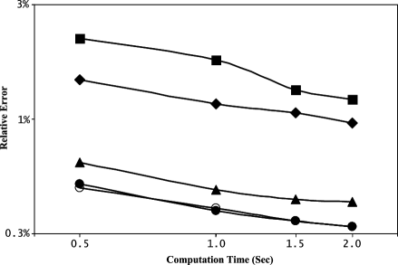
Figure 3: Plot of relative errors against computation time (sec). Both axes are in logarithmic scale. Computation time was measured on a 2.99 GHz Pentium® D CPU. Relative errors for BLOSUM45 with $\Delta(g)=14+2g$ are shown by $\blacksquare$; BLOSUM62 with $\Delta(g)=11+g$, by $\blacklozenge$; BLOSUM80 with $\Delta(g)=10+g$, by Q; PAM70 with $\Delta(g)=10+g$, by ”; PAM30 with $\Delta(g)=9+g$, by !.

Despite having the variance formula in (21) in hand, we elected to estimate the standard error $\hat{s}_{\lambda}$ directly from the 200 independent estimates $\hat{\lambda}$. Figure 3 plots the relative error $\hat{s}_{\lambda}/\bar{\lambda}$ in each individual $\hat{\lambda}$ against the computation time, where $\hat{s}_{\lambda}$ is the standard error of $\hat{\lambda}$. It shows that for all 5 BLASTP online options, (10) easily computed $\hat{\lambda}$ to 1–4% accuracy within about 0.5 seconds.

5 Discussion

This article indicates that the scale parameter $\lambda$ of the Gumbel distribution for local alignment of random sequences satisfies (10), an equation involving the strict ascending ladder-points (SALEs) from global alignment, at least approximately. For standard protein scoring systems, in fact, simulation error could account for most (if not all) of the observed differences between values of $\lambda$ calculated from (10) and values calculated from extensive crude Monte Carlo simulations. (The values of $\lambda$ from crude simulation have a standard error of about $\pm$1%.) In SALE simulations, (10) estimated $\lambda$ to 1–4% accuracy within 0.5 second, as required by BLAST database searches over the Web. The present study did not tune simulations much; it relied instead on methods specific to sequence alignment to improve estimation. Many general strategies for sequential importance sampling therefore remain available to speed simulation. Preliminary investigations estimating the other Gumbel parameter (the pre-factor $K$) with SALEs are encouraging, so online estimation of the entire Gumbel distribution for arbitrary scoring schemes appears imminent, and preliminary computer code is already in place.

Appendix: A general mapping theorem for importance sampling

The following theorem describes an unusual type of Rao-Blackwellization 35 . Consider two probability spaces $(\Omega,\mathsf{F},\mathbb{Q})$ and $(\Omega^{\prime},\mathsf{F}^{\prime},\mathbb{P})$, and a $\mathsf{F}/\mathsf{F}^{\prime}$-measurable function $f\dvtx\Omega\mapsto\Omega^{\prime}$ (i.e., $f^{-1}F^{\prime}\in\mathsf{F}$ for every $F^{\prime}\in\mathsf{F}^{\prime})$. Note: $f$ is explicitly permitted to be many-to-one. Let $\mathbb{P}<<\mathbb{Q}f^{-1}$ on some set $H^{\prime}$ (i.e., $\mathbb{Q}f^{-1}G^{\prime}=0\Rightarrow\mathbb{P}G^{\prime}=0$ for any set $G^{\prime}\subseteq H^{\prime})$, so the Radon–Nikodym derivative in the second line of (Appendix: A general mapping theorem for importance sampling) below exists. Let $H:=f^{-1}H^{\prime}$, so for every random variate $X^{\prime}$ on $(\Omega^{\prime},\mathsf{F}^{\prime})$,

$$\qquad\mathbb{E}[X^{\prime};H^{\prime}] := \int_{\omega^{\prime}\in H^{\prime}}X^{\prime}(\omega^{\prime})\,d\mathbb{P}(\omega^{\prime})$$

$$= \int_{\omega^{\prime}\in H^{\prime}}X^{\prime}(\omega^{\prime})\,d\mathbb{P}(\omega^{\prime})\int_{\omega\in f^{-1}(\omega^{\prime})}\frac{d\mathbb{Q}(\omega)}{\int_{\omega_{0}\in f^{-1}(\omega^{\prime})}\,d\mathbb{Q}(\omega_{0})}$$

$$= \int_{\omega^{\prime}\in H^{\prime}}\int_{\omega\in f^{-1}(\omega^{\prime})}X^{\prime}f(\omega)\frac{d\mathbb{P}f(\omega)}{\int_{\omega_{0}\in f^{-1}\{f(\omega)\}}\,d\mathbb{Q}(\omega_{0})}\,d\mathbb{Q}(\omega)$$

$$= \int_{\omega\in H}X^{\prime}f(\omega)\frac{d\mathbb{P}f(\omega)}{\int_{\omega_{0}\in f^{-1}\{f(\omega)\}}\,d\mathbb{Q}(\omega_{0})}\,d\mathbb{Q}(\omega).$$

Consider the application of (Appendix: A general mapping theorem for importance sampling) to importance sampling with target distribution $\mathbb{P}$ and trial distribution $\mathbb{Q}$. Assume $\mathbb{Q}H=1$, so $H$ supports $\mathbb{Q}$. In our application to global alignment, $H=[\beta(k)<\infty]\subset\Omega$ (“$\subset$” being strict inclusion), but we speculate $\mathbb{Q}H=1$.

In Monte Carlo applications, a discrete sample space $H$ is usually available. Accordingly, the following theorem replaces the integrals in (Appendix: A general mapping theorem for importance sampling) by sums.

The mapping theorem for importance sampling

Let

$$\frac{1}{W(\omega)}:=\frac{\sum_{\omega_{0}\in f^{-1}\{f(\omega)\}}\mathbb{Q}(\omega_{0})}{\mathbb{P}f(\omega)}.$$ (23)

Under the above conditions, $r^{-1}\sum_{i=1}^{r}[X^{\prime}f(\omega_{i})W(\omega_{i})]\to\mathbb{E}[X^{\prime};H^{\prime}]$ with probability $1$ and in mean (with respect to $\mathbb{Q}$), as the number of realizations $r\to\infty$.

The mapping theorem is an easy application of the law of large numbers to (Appendix: A general mapping theorem for importance sampling).

References

- (1) Aldous, D. (1989). Probability Approximations via the Poisson Clumping Heuristic, 1st ed. Springer, New York. \MR0969362
- (2) Altschul, S. F., Gish, W., Miller, W., Myers, E. W. and Lipman, D. J. (1990). Basic local alignment search tool. J. Molecular Biology 215 403–410.
- (3) Altschul, S. F., Madden, T. L., Schaffer, A. A., Zhang, J., Zhang, Z., Miller, W. and Lipman, D. J. (1997). Gapped BLAST and PSI-BLAST: A new generation of protein database search programs. Nucleic Acids Res. 25 3389–3402.
- (4) Altschul, S. F., Bundschuh, R., Olsen, R. and Hwa, T. (2001). The estimation of statistical parameters for local alignment score distributions. Nucleic Acids Res. 29 351–361.
- (5) Asmussen, S. (2003). Applied Probability and Queues. Springer, New York. \MR1978607
- (6) Arratia, R. and Waterman, M. S. (1994). A phase transition for the score in matching random sequences allowing deletions. Ann. Appl. Probab. 4 200–225. \MR1258181
- (7) Bundschuh, R. (2002). Rapid significance estimation in local sequence alignment with gaps. J. Comput. Biology 9 243–260.
- (8) Bundschuh, R. (2002). Asymmetric exclusion process and extremal statistics of random sequences. Phys. Rev. E 65 031911.
- (9) Chan, H. P. (2003). Upper bounds and importance sampling of -values for DNA and protein sequence alignments. Bernoulli 9 183–199. \MR1997026
- (10) Cinlar, E. (1975). Introduction to Stochastic Processes. Prentice Hall, Upper Saddle River, NJ. \MR0380912
- (11) Dayhoff, M. O., Schwartz, R. M. and Orcutt, B. C. (1978). A model of evolutionary change in proteins. In Atlas of Protein Sequence and Structure 345–352. National Biomedical Research Foundation, Silver Spring, MD.
- (12) Dembo, A., Karlin, S. and Zeitouni, O. (1994). Limit distributions of maximal nonaligned two-sequence segmental score. Ann. Probab. 22 2022–2039. \MR1331214
- (13) Djellout, H. and Guillin, A. (2001). Moderate deviations for Markov chains with atom. Stochastic Process. Appl. 95 203–217. \MR1854025
- (14) Galombos, J. (1978). The Asymptotic Theory of Extreme Order Statistics, 1st ed. Wiley and Sons, New York.
- (15) Gotoh, O. (1982). An improved algorithm for matching biological sequences. J. Molecular Biology 162 705–708.
- (16) Henikoff, S. and Henikoff, J. G. (1992). Amino acid substitution matrices from protein blocks. Proc. Natl. Acad. Sci. USA 89 10915–10919.
- (17) Huber, P. J. (1964). Robust estimation of a location parameter. Ann. Math. Statist. 35 73–101. \MR0161415
- (18) Karlin, S. and Altschul, S. F. (1990). Methods for assessing the statistical significance of molecular sequence features by using general scoring schemes. In Proceedings of the National Academy of Sciences of the United States of America 87 2264–2268.
- (19) Kingman, J. F. C. (1961). A convexity property of positive matrices. Quart. J. Math. Oxford 12 283–284. \MR0138632
- (20) Liu, J. S. (2001). Monte Carlo Strategies in Scientific Computing. Springer, New York. \MR1842342
- (21) Mott, R. (1999). Local sequence alignments with monotonic gap penalties. Bioinformatics 15 455–462.
- (22) Mott, R. (2000). Accurate formula for -values of gapped local sequence and profile alignments. J. Molecular Biology 300 649–659.
- (23) Olsen, R., Bundschuh, R. and Hwa, T. (1999). Rapid assessment of extremal statistics for gapped local alignment. In Proceedings of the Seventh International Conference on Intelligent Systems for Molecular Biology 211–222. AAAI Press, Menlo Park, CA.
- (24) Park, Y., Sheetlin, S. and Spouge, J. L. (2005). Accelerated convergence and robust asymptotic regression of the Gumbel scale parameter for gapped sequence alignment. J. Phys. A: Mathematical and General 38 97–108.
- (25) Seneta, E. (1981). Nonnegative Matrices and Markov Chain. Springer, New York. \MR0719544
- (26) Sheetlin, S., Park, Y. and Spouge, J. L. (2005). The Gumbel pre-factor k for gapped local alignment can be estimated from simulations of global alignment. Nucleic Acids Res. 33 4987–4994.
- (27) Siegmund, D. and Yakir, B. (2000). Approximate -values for local sequence alignments. Ann. Statist. 28 657–680. \MR1792782
- (28) Spouge, J. L. (2004). Path reversal, islands, and the gapped alignment of random sequences. J. Appl. Probab. 41 975–983. \MR2122473
- (29) Storey, J. D. and Siegmund, D. (2001). Approximate p-values for local sequence alignments: Numerical studies. J. Comput. Biology 8 549–556.
- (30) Waterman, M. S., Smith, T. F. and Beyer, W. A. (1976). Some biological sequence metrics. Adv. in Math. 20 367–387. \MR0408876
- (31) Waterman, M. S. and Vingron, M. (1994). Rapid and accurate estimates of statistical significance for sequence data base searches. Proc. Natl. Acad. Sci. USA 91 4625–4628.
- (32) Waterman, M. S. and Vingron, M. (1994). Sequence comparison significance and Poisson approximation. Statist. Sci. 9 367–381. \MR1325433
- (33) Yu, Y. K. and Altschul, S. F. (2005). The construction of amino acid substitution matrices for the comparison of proteins with nonstandard compositions. Bioinformatics 21 902–911.
- (34) Yu, Y. K. and Hwa, T. (2001). Statistical significance of probabilistic sequence alignment and related local hidden Markov models. J. Comput. Biology 8 249–282.
- (35) Zhang, Y. (1995). A limit theorem for matching random sequences allowing deletions. Ann. Appl. Probab. 5 1236–1240. \MR1384373