Electric fields in solar magnetic structures due to gradient driven instabilities: heating and acceleration of particles

Abstract

The electrostatic instabilities driven by the gradients of the density, temperature and magnetic field, are discussed in their application to solar magnetic structures. Strongly growing modes are found for some typical plasma parameters. These instabilities i) imply the presence of electric fields that can accelerate the plasma particles in both perpendicular and parallel directions with respect to the magnetic field vector, and ii) can stochastically heat ions. The perpendicular acceleration is to the leading order determined by the $\mn@boldsymbol{E}\times\mn@boldsymbol{B}$-drift acting equally on both ions and electrons, while the parallel acceleration is most effective on electrons. The experimentally confirmed stochastic heating is shown to act mainly in the direction perpendicular to the magnetic field vector and acts stronger on heavier ions. The energy release rate and heating may exceed for several orders of magnitude the value accepted as necessary for a self-sustained heating in the solar corona. The energy source for both the acceleration and the heating is stored in the mentioned background gradients.

1 Introduction

Very strong electric fields have been reported in the solar atmosphere in many studies in the past. The magnitude of such fields may amount to $7\cdot 10^{4}\;$V/m (Davis, 1977) and even up to $1.3\cdot 10^{5}\;$V/m (Zhang & Smartt, 1986). It is widely believed that these electric fields appear in the process of magnetic reconnection. The magnetic reconnection itself implies a considerable change in the magnetic field topology, and it is also used in describing rapid energy releases and ‘energization’ of plasma particles, i.e. their heating and acceleration. However, at least in some cases (Janssens, 1972; Mayfield & Chapman, 1981; Pudovkin et al., 1998) such energy release events seem to appear without a measurable change of the magnetic energy and configuration and, hence, a different description and source of such events may be needed. In the present work, we show that such an alternative source naturally exists, and that it may drive extremely strong electrostatic instabilities and produce electric fields of the order mentioned above. The energy for such instabilities is provided by the omnipresent gradients of the background plasma parameters (the density, temperature, and magnetic field). However, the physics and the features of this source, and the mechanism by which its energy is transferred into these instabilities are beyond the standard magnetohydrodynamics (MHD) model. In order to describe it, a multi-component (fluid or kinetic) theory is needed.

Typical studies of oscillations and instabilities in the solar magnetic field structures imply a cylindric geometry with parameters having different values inside and outside of the structure, yet having at the same time some constant values in the two separate domains. Moreover, the usually curved structures (e.g. magnetic loops) are often flattened out in the modeling and the curvature effects are thus neglected in the simplified models. In reality however, the plasma parameters (the density, temperature and magnetic field magnitude) may vary both in the axial (parallel to the magnetic field vector) and in the radial (perpendicular) direction. The axial variation is typically on a much larger characteristic spatial scale in comparison to the radial variation, and in some cases can be omitted. The presence of these radial inhomogeneities in the background of some accidental fluctuations implies a source of energy for certain types of instabilities. These background (equilibrium) gradients also imply the equilibrium drift velocities, and the associated instabilities are usually termed as reactive drift instabilities, first predicted long ago by Rudakov & Sagdeev (1961). A drift wave driven by the density gradient is typically growing due to the electron thermal effects in both collisional and collision-less regimes (Vranjes & Poedts, 2006, 2009a, 2009b). The former is well described within the two-component fluid theory, the latter however, is a strictly kinetic effect. In both cases the ions play a stabilizing role, and in some situations they may even impose a threshold for the instability.

However, in the case of hot ions and in the presence of both the density and temperature gradients, the above mentioned reactive instability is termed as $\eta_{i}$-instability, where now the ions play a crucial destabilizing role. Here, $\eta_{i}=L_{n}/L_{\scriptscriptstyle T}$, and $L_{n}=(dn_{0}/dx/n_{0})^{-1}$, $L_{\scriptscriptstyle T}=(dT_{0}/dx/T_{0})^{-1}$ are the characteristic inhomogeneity scale-lengths of the equilibrium quantities that are here, and further in the text, denoted by the index 0. The coordinate $x$ in the present local analysis is used to describe the changes in the radial (perpendicular) direction. The background magnetic field is typically also inhomogeneous (i.e., with a curvature and a gradient in the perpendicular direction), and this may be described by yet another characteristic scale-length $L_{\scriptscriptstyle B}=(dB_{0}/dx/B_{0})^{-1}$. The interplay of these three gradients determines the behavior of low frequency ($\omega\ll\Omega_{i}=q_{i}B_{0}/m_{i}$, $q_{i}=Z_{i}e$ is the ion charge) electrostatic oscillations and instabilities. This will be demonstrated in the forthcoming text.

2 Electrostatic instability in an advanced fluid model

We apply the two-fluid model developed in numerous works related to laboratory plasmas (Nilsson et al., 1990; Nilsson & Weiland, 1995). A systematic presentation of the theory that has been successfully used in the past in the prediction of transport processes in tokamak plasmas can be found in Weiland (2000). There, one can also see a complete agreement between this advanced fluid model and the kinetic theory (that is one of the reasons for the term ‘advanced’ used here). Part of the basic theory of the drift wave applied to the solar plasmas is given in Vranjes & Poedts (2006). It has also been used very recently (Vranjes & Poedts, 2009a, b) in order to explain some essential properties of the coronal heating mechanism. The theory is described in detail in the references mentioned above. For completeness, we shall provide here a general description of the derivations, emphasizing some most important features of the model and providing explanations for the assumptions used in the procedure. The present analysis is restricted to the electrostatic limit. Note however, that the theory works well also in the full electromagnetic limit (Andersson & Weiland, 1988), where it can be used e.g. for describing the ballooning instabilities. This domain also can be of great importance for the solar plasma as it may provide a triggering mechanism for abrupt changes in the magnetic field topology, e.g. in processes like magnetic reconnection and Coronal Mass Ejections (CMEs).

The presence of hot ions (typical for the solar atmosphere) and the background temperature gradient (that is expected in solar magnetic configurations) implies, first of all, the necessity of including their full thermal response (the pressure and the gyro-viscosity collision-less stress tensor) in the momentum equation, and, second, the use of the ion energy equation in the mathematical model. For the present purpose, the later comprises the diamagnetic heat flow term only, and can be written as (Weiland, 2000)

$$\frac{3}{2}n_{i}\left(\frac{\partial}{\partial t}+\mn@boldsymbol{v_{i}}\cdot\nabla\right)T_{i}+p_{i}\nabla\cdot\mn@boldsymbol{v_{i}}=-\nabla\cdot\mn@boldsymbol{q_{*i}},$$ (1)

$$\mn@boldsymbol{q_{*i}}=\frac{5}{2}\frac{n_{i}T_{i}}{m_{i}\Omega_{i}}\mn@boldsymbol{e_{\|}}\times\nabla T_{i}.$$

Here, $T_{i}$ is in energy units, $\mn@boldsymbol{q_{*i}}$ is the diamagnetic heat flux, and $\mn@boldsymbol{e_{\|}}=\mn@boldsymbol{B}/B$. The given form of $\mn@boldsymbol{q_{*i}}$ can be obtained directly from the drift-kinetic theory. In the case of different temperatures (pressures) in the two directions (Mondt & Weiland, 1991) it is to be replaced with $[p_{i\bot}/(m_{i}\Omega_{i})]\mn@boldsymbol{e_{\|}}\times\nabla(2T_{i\bot}+T_{i\|}/2)+[(p_{i\|}-p_{i\bot})/(m_{i}\Omega_{i})]T_{i\|}\mn@boldsymbol{e_{\|}}\times(\mn@boldsymbol{e_{\|}}\cdot\nabla)\mn@boldsymbol{e_{\|}}$. A detailed analysis of the temperature anisotropy effects on the gradient driven instability is performed by Mondt (1996).

The magnetic field is inhomogeneous in the general case. This implies that, in the continuity equation, the contribution of the diamagnetic drift to the ion flux does not vanish, and the appropriate linearized term is

$$\nabla\cdot(n_{i}\mn@boldsymbol{v_{*i}})=\frac{1}{T_{i}}\mn@boldsymbol{v_{bi}}\cdot\nabla p_{i1}\neq 0.$$

For the same reason we have also $\nabla\cdot\mn@boldsymbol{v_{\scriptscriptstyle E}}\neq 0$, where $\mn@boldsymbol{v_{\scriptscriptstyle E}}$ is the $\mn@boldsymbol{E}\times\mn@boldsymbol{B}$-drift. Hence, an additional magnetic drift velocity $\mn@boldsymbol{v_{bi}}$ appears in the description of the ion motion. We use standard notation from the drift wave theory where $\mn@boldsymbol{v_{*i}}=\mn@boldsymbol{e_{\|}}\times\nabla p_{i}/(q_{i}n_{i}B)$. In the equations above we have $\nabla\cdot\mn@boldsymbol{q_{*i}}=-5n_{i}v_{*i}\nabla T_{i}/2+5n_{i}\mn@boldsymbol{v_{bi}}\cdot\nabla T_{i}/2$. The first (non-curvature) part in this expression cancels out in the procedure of calculating $\nabla\cdot\mn@boldsymbol{v_{i}}$ in the ion continuity equation. The second term comprises the ion magnetic drift, which in the general case is the sum of the curvature and the gradient-$B$ drifts

$$\mn@boldsymbol{v_{bi}}=\frac{v_{\|}^{2}}{\Omega_{i}}\mn@boldsymbol{e_{\|}}\times(\mn@boldsymbol{e_{\|}}\cdot\nabla)\mn@boldsymbol{e_{\|}}+\frac{v_{\bot}^{2}}{2\Omega_{i}}\mn@boldsymbol{e_{\|}}\times\nabla\log B.$$

Here, $(\mn@boldsymbol{e_{\|}}\cdot\nabla)\mn@boldsymbol{e_{\|}}=-\mn@boldsymbol{R}/R^{2}$ and $R$ denotes the radius of the curvature of the magnetic field, while the two velocities are in general case different $v_{\|}^{2}=T_{i}/m_{i}$, $v_{\bot}=2T_{i}/m_{i}$. In what follows, we shall use the expression for the effective total curvature drift (Weiland, 2000) $\mn@boldsymbol{v_{bi}}\simeq[2T_{i0}/(q_{i}B_{0})]\mn@boldsymbol{e_{\|}}\times(\mn@boldsymbol{e_{\|}}\cdot\nabla)\mn@boldsymbol{e_{\|}}$.

Figure 1: Contour plot of $F(L_{n},L_{\scriptscriptstyle T},L_{\scriptscriptstyle B})=\eta_{i}-\eta_{th}$, for $k_{y}\rho_{s}=0.1$. The positive values correspond to the instability.

The perturbed ion perpendicular velocity can be obtained from the ion momentum equation by applying the vector product $\mn@boldsymbol{e_{\|}}\times...$, yielding

$$\mn@boldsymbol{v_{i\bot}}=\mn@boldsymbol{v_{\scriptscriptstyle E}}+\mn@boldsymbol{v_{*i}}+\mn@boldsymbol{v_{pi}}+\mn@boldsymbol{v_{\pi i}}.$$ (2)

Here, $\mn@boldsymbol{v_{\scriptscriptstyle E}}$ and $\mn@boldsymbol{v_{*i}}$ are already defined above, the third term is the ion polarization drift, and $\mn@boldsymbol{v_{\pi i}}$ denotes the drift due to the ion stress tensor effects. For small accidental perturbations propagating predominantly in the perpendicular direction $\sim\exp[-i\omega t+ik_{y}y+ik_{z}z]$, $|k_{y}|\gg|k_{z}|$, $|\omega|\ll\Omega_{i}$, the linearized ion energy equation yields (Weiland, 2000)

$$\frac{T_{i1}}{T_{i0}}=\frac{\omega}{\omega-5\omega_{bi}/3}\left[\frac{2}{3}\frac{n_{i1}}{n_{0}}+\frac{\omega_{*e}}{\omega}\left(\eta_{i}-\frac{2}{3}\right)\frac{e\phi_{1}}{T_{e0}}\right].$$

Here, the terms $\omega_{*j}$, $\omega_{bj}$ are the product of the perpendicular wave number component $k_{y}$ and the diamagnetic and magnetic drifts, respectively. Note that $\omega_{*e}=k_{y}v_{*e}=-\tau\omega_{*i}$, $\tau=T_{e0}/T_{i0}$. Using Eq. (2) in the ion continuity, the ion density perturbation can be written as (Weiland, 2000):

$$\frac{n_{i1}}{n_{0}}=\left\{\omega(\omega_{*e}-\omega_{be})+\left(\eta_{i}-\frac{7}{3}+\frac{5\eta_{b}}{3}\right)\omega_{*e}\omega_{bi}\right.$$

$$\left.-k_{y}^{2}\rho_{s}^{2}\left[\omega-\omega_{*i}(1+\eta_{i})\right]\left(\omega-\frac{5\omega_{bi}}{3}\right)\right\}$$

$$\times\left[\omega^{2}-\frac{10\omega\omega_{bi}}{3}+\frac{5\omega_{bi}^{2}}{3}\right]^{-1}\frac{e\phi_{1}}{T_{e0}}.$$ (3)

The electron parallel dynamics yields just the Boltzmann distribution for the electron number density, and using the quasi-neutrality condition, one then obtains the dispersion equation

$$\Omega^{2}\left(1+k_{y}^{2}\rho_{s}^{2}\right)+\Omega\left[\frac{10\eta_{b}}{3\tau}+k_{y}^{2}\rho_{s}^{2}\frac{5\eta_{b}}{3\tau}-1+\eta_{b}+k_{y}^{2}\rho_{s}^{2}\frac{1+\eta_{i}}{\tau}\right]$$

$$+\frac{5\eta_{b}^{2}}{3\tau^{2}}+\left(\eta_{i}-\frac{7}{3}+\frac{5\eta_{b}}{3}\right)\frac{\eta_{b}}{\tau}+k_{y}^{2}\rho_{s}^{2}\frac{1+\eta_{i}}{\tau}\frac{5\eta_{b}}{3\tau}=0.$$ (4)

Here, $\Omega\equiv\omega/\omega_{*e}$, $\rho_{s}=c_{s}/\Omega_{i}$, $c_{s}^{2}=T_{e0}/m_{i}$, $\eta_{b}=\omega_{bi}/\omega_{*i}=L_{n}/L_{\scriptscriptstyle B}$, and $\omega_{be}=-\tau\omega_{bi}$. It is seen that, without the magnetic field inhomogeneity, Eq. (4) yields only the standard drift mode driven by the density gradient, with $\omega\sim 1/L_{n}$. The magnetic drift terms $\omega_{bi}$ are responsible for the appearance of the additional plasma mode, while all three gradients together are responsible for the instability. As shown by Weiland (2000), Eq. (4) can be solved analytically yielding the approximate growth-rate (normalized to $\omega_{*e}$)

$$\gamma=\frac{(\eta_{b}/\tau)^{1/2}}{1+k_{y}^{2}\rho_{s}^{2}}(\eta_{i}-\eta_{th})^{1/2},$$

$$\eta_{th}=\frac{2}{3}-\frac{\tau}{2}+\eta_{b}\left(\frac{\tau}{4}+\frac{10}{9\tau}\right)+\frac{\tau}{4\eta_{b}}-\frac{k_{y}^{2}\rho_{s}^{2}}{2\eta_{b}}\left[\frac{5}{3}-\frac{\tau}{4\eta_{b}}\right.$$

$$\left.+\frac{\tau}{4\eta_{b}}-\left(\frac{10}{3}+\frac{\tau}{4}-\frac{10}{9\tau}\right)\eta_{b}+\left(\frac{5}{3}+\frac{\tau}{4}-\frac{10}{9\tau}\right)\eta_{b}^{2}\right].$$

Figure 2: Two real solutions (normalized to $\omega_{*e}$) in the case $\eta_{i}=1$ and $k_{y}\rho_{s}=0.1$.

It is seen that for $\eta_{i}>\eta_{th}$ there will be an instability. For a fixed $\tau$, the stability conditions are completely determined by the three characteristic inhomogeneity scale-lengths $L_{n},L_{\scriptscriptstyle T},L_{\scriptscriptstyle B}$. This is demonstrated in Fig. 1 where we give the contour plot of $F(L_{n},L_{\scriptscriptstyle T},L_{\scriptscriptstyle B})=\eta_{i}-\eta_{th}$ for $k_{y}\rho_{s}=0.1$ and for $\tau=T_{e0}/T_{i0}=1$. The positive lines denote the values for which the gradient-driven instability takes place. In application to the solar atmosphere with $T_{e0}=T_{i0}=10^{6}\;$K, and assuming $B_{0}=3\cdot 10^{-2}\;$T, for hydrogen ions we have $\rho_{s}=0.032\;$m and, hence, the condition $k_{y}\rho_{s}=0.1$ implies the perpendicular wavelength $\lambda_{y}=2\;$m. The assumption of the nearly perpendicular perturbed ion motion for such a short perpendicular wave-length in fact implies a flute-like mode that is very elongated along the magnetic field vector, with a parallel wave-length that is measured in hundreds of kilometers. Such strongly elongated modes (i.e. $k_{\bot}\gg k_{\|}$) are easily excited under laboratory conditions (e.g. in a tokamak plasma) in spite of the rather limited scales in the parallel direction. In the solar magnetic structures with naturally drastic differences in the perpendicular and parallel scale-lengths, their excitation is expected to be even more efficient.

The second order dispersion equation (4) is solved numerically and some results are presented in Figs. 2-5. In accordance with Fig. 1, in Fig. 2 for $\eta_{i}=1$ we have two real solutions for the wave frequency, one essentially due to the density gradient and the other due to the magnetic field gradient. The initially positive solution changes the sign for $\eta_{b}\simeq 0.4$ and then both solutions propagate in the direction of the ion diamagnetic drift. Note that for the parameters used above and for $k_{y}\rho_{s}=0.1$, the normalized frequency $\Omega\sim 1\;$Hz here implies $L_{n}=L_{\scriptscriptstyle T}\sim 10^{3}\;$m.

In Fig. 3, the case $\eta_{i}=3$ is presented. Here, both initial solutions are positive and real for small values of $\eta_{b}$. They merge at around $\eta_{b}\simeq 0.09$, yielding a pair of complex-conjugate solutions with the real part becoming negative for $\eta_{b}>0.25$. The instability vanishes for $\eta_{b}>2.04$ when two negative real solutions appear. The mode is particularly strongly growing ($|\gamma|>|\Omega_{r}|$) in the range $\eta_{b}\in(0.15,\,0.7)$.

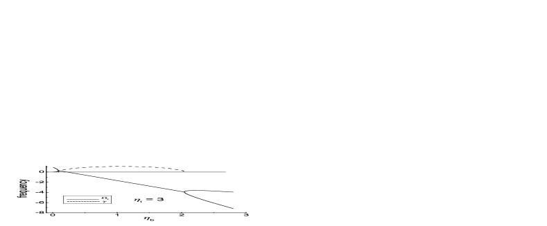
Figure 3: The solutions of Eq. (4) for $\eta_{i}=3$ showing two real solutions for small $\eta_{b}$ and for $\eta_{b}>2.04$. The dashed line is the growth-rate for the complex-conjugate solutions in between.

Figure 4: The solutions of Eq. (4) for $\eta_{i}=5$.

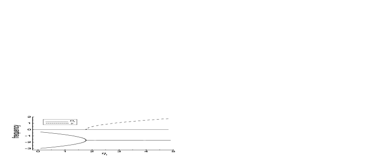
Figure 5: The solutions of Eq. (4) in terms of $\eta_{i}$ for $\eta_{b}=1$.

Considering $\eta_{i}=5$, in Fig. 4 we present the same mode behavior as in Fig. 3. Such a larger $\eta_{i}$ value yields a growth-rate that is larger by about a factor 2 and the instability range in terms of $\eta_{b}$ is widened to $\eta_{b}\in(0.05,\,3.7)$.

In Fig. 5, for a fixed $\eta_{b}=1$ and $k_{y}\rho_{s}=0.1$, the frequency is calculated in terms of $\eta_{i}$. The two negative real solutions (c.f. Fig. 2) merge for $\eta_{i}\geq 1.78$ yielding a pair of complex conjugate solutions with a very weakly decreasing real part ($\Omega_{r}=-1.67$ at $\eta_{i}=1.78$ and $\Omega_{r}=-1.71$ at $\eta_{i}=10$).

Note that in all these cases the used values of the ratios $\eta_{i}\equiv L_{n}/L_{\scriptscriptstyle T}$, $\eta_{b}\equiv L_{n}/L_{\scriptscriptstyle B}$ in fact imply a wide range of possible values for $L_{n},\,L_{\scriptscriptstyle T},L_{\scriptscriptstyle B}$. Since $\omega_{r}=\Omega_{r}\omega_{*e}\sim 1/L_{n}$, this also implies a wide range of possible frequencies.

3 Electric field

3.1 Acceleration of plasma particles

The electrostatic instability discussed here implies an electric field varying in time and space, and having very different components in the parallel and perpendicular directions. Such an electric field can accelerate plasma particles in both perpendicular and parallel directions with respect to the magnetic field vector. An acceleration always exists in the presence of electrostatic perturbations, yet typically it is sporadic and acts mainly on the small amount of particles from the far tail in the distribution function. The critical value of such an electric field, above which the bulk electron runaway effect takes place, in a fully ionized plasma is (Dreicer, 1959) $E_{d}=eL_{ei}/(4\pi\varepsilon_{0}\lambda_{d}^{2})$. Here, $L_{ei}=\log(\lambda_{d}/b)$ is the Coulomb logarithm, $\lambda_{d}=\lambda_{de}\lambda_{di}/(\lambda_{de}^{2}+\lambda_{di}^{2})^{1/2}$ is the plasma Debye radius, $\lambda_{dj}=v_{{\scriptscriptstyle T}j}/\omega_{pj}$, $v_{{\scriptscriptstyle T}j},\omega_{pj}$ are, respectively, the thermal velocity and the plasma frequency of the $j$ species, and $b=[e^{2}/[12\pi\varepsilon_{0}(T_{e}+T_{i})]$ is the impact parameter for electron-ion collisions. For the parameters used in the previous text we have $L_{ei}=19$, $\lambda_{d}=0.0005\;$m, and the Dreicer field is $0.11\;$V/m. Assuming the parallel wave-length of about $100(500)\;$km, the amplitude of the electrostatic potential $\phi$ necessary to achieve the Dreicer value is about $1.8(9)\;$KV. However, in the perpendicular direction this same potential gives the electric field $k_{y}\phi$ that is around $E_{\bot}=5.7(29)\;$KV/m. For the parallel wave-length of about $1000\;$km we would have $\phi=18\;$KV and consequently $E_{\bot}=57\;$KV/m. These estimates are for the number density $n_{0}=10^{16}\;$m^-3.

Figure 6: The threshold value of the potential $\phi$, Eq. (5), in terms of the perpendicular wave-length, above which the stochastic heating takes place. Above the dotted line the parallel electric field exceeds the Dreicer value, resulting in a simultaneous acceleration of particles.

Table 1: Stochastic heating for hydrogen (and helium in brackets) for several values of the perpendicular wavelength and the wave amplitude $\phi$. The assumed starting temperature is $10^{6}$ K.

$\lambda_{y}$ [m]	$\phi$ [V]	$a$	$T_{eff}$ [K]
0.1	$50$	$2.3$ $(9.1)$	$1.5\cdot 10^{6}$ $(2.6\cdot 10^{6})$
0.2	$100$	$1.1$ $(4.6)$	$3\cdot 10^{6}$ $(3.5\cdot 10^{6})$
1	$3000$	$1.4$ $(5.5)$	$9\cdot 10^{7}$ $(1.2\cdot 10^{8})$
1	$5000$	$2.3$ $(9.1)$	$1.5\cdot 10^{8}$ $(2.6\cdot 10^{8})$
2	$10000$	$1.1$ $(4.6)$	$3.1\cdot 10^{8}$ $(3.5\cdot 10^{8})$

Taking the number density one order of magnitude larger $n_{0}=10^{17}\;$m^-3 yields $E_{d}=1\;$V/m. The electric field corresponding to this value in the parallel direction would (for the three given parallel wavelengths) in the perpendicular direction have the magnitude of $54$, $270$, and $540\;$kV/m, respectively.

The time needed for the perturbations to achieve such values can be estimated from the previously calculated growth-rates. Taking as an example Fig. 3, the maximum growth-rate is $\gamma/\omega_{*e}\simeq 1$. Taking $L_{n}=10^{3}\;$m, $T_{i}=T_{e}=T_{0}=10^{6}\;$K, $B_{0}=3\cdot 10^{-2}\;$T, for $\lambda_{y}=2\;$m we have $\omega_{*e}=9\;$Hz. Assuming some small starting value of the electrostatic potential $\Psi$, the growth time till it gets some value $\phi_{1}$ is $t_{g}\simeq\log(\phi_{1}/\Psi)/\gamma$. Taking $e\Psi/(\kappa T_{i})=0.01$ this yields $\Psi=0.86\;$V. Hence, the value $\phi_{1}=9\;$KV discussed above is achieved within $t_{g}\simeq 1\;$s. Observe that for $L_{n}=10^{4}\;$m, this growth time becomes $10$ seconds.

We conclude that the presented instability can yield the extremely large values of the electric field reported in the observations (Davis, 1977; Zhang & Smartt, 1986) within seconds. The electric field generated in such a way may exceed the Dreicer value, and consequently an acceleration of the bulk plasma may take place. In the direction perpendicular to the magnetic field vector, the particles are subject to the leading order $\mn@boldsymbol{E}\times\mn@boldsymbol{B}$-drift $v_{\scriptscriptstyle E}=E_{\bot}/B_{0}$, which is the same for both electrons and ions. Note that for $E_{\bot}=20\;$KV/m and the earlier assumed magnetic field, it is of the order of $700\;$km/s. Hence, because of such short perpendicular wave-lengths, these are very short-scale perpendicular plasma fluxes acting on the plasma as a whole.

The nature of the instability is that in the perpendicular direction (here along the $x$-axis) it is localized in the area of the maximum gradients e.g. around some value $x_{0}$. On the other hand, the perpendicular component of the perturbed electric field is in the $y$-direction (corresponding to the azimuthal direction in the cylindric geometry), so that due to the $\mn@boldsymbol{E}\times\mn@boldsymbol{B}$-drift the plasma fluxes will be in the $x$-direction. Hence, the starting regular density profile in the $x$-direction will be modified and density condensations will appear one after another as one moves in the $y$-direction, left and right of the position $x_{0}$. In a realistic cylindric geometry and taking the mode behavior in the axial direction into account, this would imply the formation of braided density structures twisted along the cylinder. However, in the limit of large potential amplitudes the initial plasma configuration can simply be destroyed.

In the parallel direction the velocity (Bittencourt, 1995; Vranjes & Poedts, 2009b) is $v_{jz}(t)\sim E_{z}/[m_{j}(k_{z}v_{0}-\omega_{r})]$. Hence, the acceleration is proportional to $m_{j}^{-1}$ and acts mainly on electrons. It is selective in the sense that particularly strong acceleration is experienced by resonant electrons having the starting velocity $\mn@boldsymbol{v_{0}}$ satisfying the condition $v_{0z}=\omega_{r}/k_{z}$. More details on that issue may be found in Fletcher & Hudson (2008) and Vranjes & Poedts (2009b).

3.2 Quasi-static purely growing instability

The instability described in the previous text implies the presence of a range of values for the three parameters $L_{n},L_{\scriptscriptstyle T},L_{\scriptscriptstyle B}$ for which $|\Omega_{r}|\ll\gamma$. This is due to the demonstrated change of the mode direction, during which the dispersion lines intersect with the $\eta_{b}$-axis so that $\omega_{r}=0$. In Figs. 3 and 4 this is around $\eta_{b}\simeq 0.25$. The corresponding growth-rate for the two cases is $\gamma\simeq 0.6$ and $0.9$, respectively.

This implies an almost purely growing, quasi-static electric field, yet spatially varying and with its amplitude determined by the the two mode numbers $k_{y,z}$. The above described acceleration will remain similar, yet the important difference is that the mode is practically non-propagating and the spatial variation of the acceleration will become much more pronounced and the mentioned braiding more effective.

3.3 Stochastic heating

The polarization drift, i.e. the third term in Eq. (2), starts to play an important role for a large enough wave amplitude. In this case, the motion of a particle becomes stochastic and consequently heating takes place. Details of this process can be found in Bellan (2006). It turns out that for a large enough wave amplitude the standard iterative procedure, which is behind Eq. (2), is not valid any more, and the same holds for the particle representation by its gyro-center. Instead, one is supposed to describe the actual particle motion by writing the particle momentum equation for its motion in the wave-field. This has been described in detail and experimentally verified in McChesney et al. (1987) and Sanders et al. (1998). It is shown that the stochastic heating takes place provided that

$$a=k_{y}^{2}\rho_{i}^{2}\cdot\frac{e\phi}{T_{i0}}\geq 1.$$ (5)

Here, $\rho_{i}=v_{{\scriptscriptstyle T}i}/\Omega_{i}$. The condition (5) in fact implies that in this regime the ion displacement due to the polarization drift is comparable to the perpendicular wavelength. This is because $\mn@boldsymbol{v_{pi}}=(\mn@boldsymbol{e_{z}}\times\partial\mn@boldsymbol{v_{i\bot}}/\partial t)/\Omega_{i}$, and $\mn@boldsymbol{v_{i\bot}}$ is the leading order $\mn@boldsymbol{E}\times\mn@boldsymbol{B}$-drift, so that (McChesney et al., 1987) $v_{pi}\sim a\omega/k_{y}$ and the perpendicular displacement due to the polarization drift is $\delta=v_{pi}/\omega=a/k_{y}$. For these reasons the mentioned gyro-center representation fails and the field magnitude is to be calculated at the actual position of the particle. Another important feature is that $\mn@boldsymbol{v_{pi}}\sim\mn@boldsymbol{k_{y}}$, hence the stochastic heating is due to the electrostatic property of the wave. Although the resulting particle motion is deterministic, as explained in Bellan (2006) the practical consequence of the described mechanism on the particle distribution function is the same as in an ordinary heating.

The maximum achieved stochastic temperature is (McChesney et al., 1987; Sanders et al., 1998)

$$T_{max}=\frac{m}{3}\left(k_{y}^{2}\rho_{i}^{2}e\phi/T_{i0}+1.9\right)^{2}\frac{\Omega_{i}^{2}}{k_{y}^{2}}.$$ (6)

The application of this effect to the heating of the solar corona by the ordinary density gradient driven drift wave has been performed in our recent publications Vranjes & Poedts (2009a) and Vranjes & Poedts (2009b). It is shown that the ions are more efficiently heated than electrons, and the heavier ions are heated better than light ions provided that $k_{y}^{4}\rho_{i}^{4}(e\phi/T_{i0})^{2}>1.9$. The nature of the heating is such that it acts mainly in the perpendicular direction, and it can also describe some other features of the coronal heating.

The threshold potential (5) is presented in Fig. 6 in terms of $\lambda_{y}$, for the same parameters as earlier in the text. For the values above the curve, the stochastic heating takes place. On the other hand, as discussed earlier in the text, for large enough $k_{z}\phi$ the electric field exceeds the Dreicer value and the particle acceleration is in action too. The horizontal lines in Fig. 6 give $k_{z}\phi=E_{d}$ for the cases $\lambda_{z}=100\;$km and $500\;$km. Hence, for the values of $\phi$ above the both full and dotted lines, the plasma is subject to simultaneous heating of ions (in the perpendicular direction), and an acceleration of bulk electrons in the parallel direction.

The stochastic temperature (6) is sensitive to the perpendicular wavelength and the magnitude of the background magnetic field. Using the parameters from the previous text and the starting temperature of $1\;$MK one can easily obtain a temperature several orders of magnitude above the starting value, and this already for a very small amplitude of the potential $\phi$. The heating presented in Table 1 is for rather moderate values of the perturbed potential, i.e., for the left (lower) part of the curve in Fig. 6. From Table 1, one concludes that at very short perpendicular wave-lengths, the stochastic heating is in action already at very small amplitudes of the wave potential. Also clear from Table 1 is the remarkable fact that for the same wave amplitude the heavier ions (helium) are heated more efficiently.

The stochastic heating implies the condition (5) satisfied, regardless of the specific values of the two separate parts in that expression, while the instability analysis and the growth-time from Sec. 2 imply $k_{y}\rho_{s}\equiv k_{y}\rho_{i}<1$. For that reason we are formally allowed to estimate the growth time in Table 1 for $\lambda_{y}\geq 2\;$m only, and this is of the order of a second, as shown in Sec. 3.1. For this wave-length the maximum energy release rate per unit volume for the density $n_{0}=10^{16}\;$m^-3 becomes $3n_{0}T_{max}/(2t_{g})=65\;$J/(m³s), and that is several orders of magnitude above the value accepted as necessary for a sustained heating in coronal loops and also well within the range of the total amount of the energy released in nano-flares. Some additional properties of the stochastic heating, presented in Vranjes & Poedts (2009a) and Vranjes & Poedts (2009b) for the ordinary drift wave, remain valid for the present case as well.

Summary

The heating of the solar corona by waves, and the propagation of waves in the solar environment has been the subject of numerous studies in the past. Typically the wave heating models remain within the widely used MHD, e.g. Pekünlü et al. (2001); Suzuki (2004), yet it is obvious that in such an approach a lot of physics remains out of scope as may be seen in Vranjes & Poedts (2006); Pandey & Wardle (2008). The analysis performed in the present paper is aimed at showing even further some novel phenomena that follow from a multi-component description. It is based on the well established theory of the low frequency phenomena in magnetized and inhomogeneous plasmas. It is crucially a multi-component plasma description. In the same time, it represents a step forward in the recently published modeling of the heating of the solar corona (Vranjes & Poedts, 2009a, b). The most important consequence of the here described fast growing mode is the electric field, with its drastically different scales in the parallel and perpendicular directions, that cannot be predicted within the widely used MHD theory. This electric field should be responsible for the acceleration of plasma particles and their simultaneous heating. The nature of the instability implies large scales in the direction of the magnetic field vector. In a realistic cylindric configuration the mode is weakly twisted around a magnetic loop, and such is the scene where the predicted acceleration and heating takes place. The essential difference between the instability presented here and the drift wave instability from Vranjes & Poedts (2009a, b) is that the former can be well described within the multi-component fluid theory, while the latter is a purely kinetic effect.

The gradient driven oscillations presented here are of relatively high frequency and therefore presently difficult to detect directly. Yet, they imply the presence of the electric fields that can be observed in coronal spectra due to line broadening and shifts, that are measured and presented in Davis (1977) and Zhang & Smartt (1986), and attributed to plasma waves and instabilities, in particular to the lower-hybrid-drift and whistler instabilities. We show here that they can be described in terms of the gradient-driven drift instabilities. The possible consequences of the presence of gradient driven oscillations (the temperature anisotropy and a stronger heating of heaver ions) are well documented in the measurements of the spectral line widths of heavy ions Cranmer et al. (2008). The mentioned strong $\mn@boldsymbol{E}\times\mn@boldsymbol{B}$-plasma drifts should also be detectable as Doppler shifts in the spectra.

One can with certainty claim that, at least in the starting stages of the presented gradient-driven instability, these processes are reasonably accurately described within the given model that can potentially be used for the description of the particle acceleration and the heating of the solar corona. However, there exists a number of phenomena that will mostly negatively affect the proposed effects of heating and acceleration, like the energy and particle diffusion and collisions, coupling to the Alfvén wave, non-linearity, etc. Large wave amplitudes and the corresponding stronger heating will necessarily modify the starting plasma configuration, primarily the temperature gradient that is essential for the growth, and the density gradient too. Consequently, the values obtained here analytically may be far from accurate. In particular, for large values of $e\phi/(\kappa T_{i})$, various new effects must be included, and the model must be considerably improved in order to give accurate estimates in this limit. Though, the effective temperature presented in Table 1 goes over 300 million K, that is far above the temperatures that are needed. Hence, reducing the potential [i.e. the factor $e\phi/(\kappa T_{i})$] by two order of magnitude will still give desired temperature of a few million K. Such a reduction of $\phi$ will give lower values of the electric field $k_{y}\phi$, yet this can be compensated by taking larger values of $k_{y}$. For the given plasma parameters, the plasma Debye radius is around 0.5 mm, so that going to very short perpendicular wavelengths, even below the values from Table 1 is justified. Nevertheless, it is fair to say that a realistic (non-linear) development of the instability and of all the consequences that follow from it, can be described only numerically in codes that allow for a simultaneous change of the driving force (i.e., the inhomogeneous plasma background) in the process of the development of the instability.

References

- Andersson & Weiland (1988) Andersson, P., Weiland, J., 1988, Phys. Fluids, 31, 359
- Bellan (2006) Bellan, P. M., 2006, Fundamentals of Plasma Physics. Cambridge Univ. Press, Cambridge, UK
- Bittencourt (1995) Bittencourt, J. A., 1995, Fundamentals of Plasma Physics. Sao José dos Campos, Brazil
- Cranmer et al. (2008) Cranmer, S. R., Panasyuk, A. V., Kohl, J. L., 2008, ApJ, 678, 1480
- Davis (1977) Davis, W. D., 1977, Solar Phys., 54, 139
- Dreicer (1959) Dreicer, H., 1959, Phys. Rev., 115, 238
- Fletcher & Hudson (2008) Fletcher, L., Hudson, H. S., 2008, ApJ, 675, 1645
- Janssens (1972) Janssens, T. J., 1972, Solar Phys., 27, 149
- Mayfield & Chapman (1981) Mayfield, E. B., Chapman, G. A., 1981, Solar Phys., 70, 351
- McChesney et al. (1987) McChesney, J. M., Stern, R. A., Bellan, P. M., 1987, Phys. Rev. Lett., 59, 1436
- Mondt & Weiland (1991) Mondt, J. P., Weiland, J., 1991, Phys. Fluids B, 3, 3248
- Mondt (1996) Mondt, J. P., 1996, Phys. Plasmas, 3, 939
- Nilsson et al. (1990) Nilsson, J., Liljestrom, M., Weiland, J., 1990, Phys. Fluids B, 2, 2568
- Nilsson & Weiland (1995) Nilsson, J., Weiland, J., 1995, Nucl. Fuison, 35, 497
- Pandey & Wardle (2008) Pandey, B. P., Wardle, M., 2008, MNRAS, 385, 2269
- Pekünlü et al. (2001) Pekünlü, E. R., Çakirli, Ö, Özetken, E., 2001, MNRAS, 326, 675
- Pudovkin et al. (1998) Pudovkin, M. I., Zaitseva, S. A., Shumilov, N. O., Meister, C. V., 1998, Solar Phys., 178, 125
- Rudakov & Sagdeev (1961) Rudakov, L. I., Sagdeev, R. Z., 1961, Sov. Phys. Dokl., 6, 415
- Sanders et al. (1998) Sanders, S. J., Bellan, P. M., Stern, R. A., 1998, Phys. Plasmas, 5, 716
- Suzuki (2004) Suzuki, T. K., 2004, MNRAS, 349, 1227
- Vranjes & Poedts (2006) Vranjes, J., Poedts, S., 2006, A&A, 458, 635
- Vranjes & Poedts (2009a) Vranjes, J., Poedts, S., 2009a, EPL, 86, 39001
- Vranjes & Poedts (2009b) Vranjes, J., Poedts, S., 2009b, MNRAS (to be published)
- Weiland (2000) Weiland, J., 2000, Collective Modes in Inhomogeneous Plasmas. Institute of Physics Pub., Bristol, Uk
- Zhang & Smartt (1986) Zhang, Z., Smartt, R. N., 1986, Solar Phys., 105, 355