Spatial correlators in strongly coupled plasmas

Abstract:

We numerically calculate the spatial correlators of the scalar and pseudoscalar operators $F^{2}$ and $F\tilde{F}$, in SU(3) Yang-Mills theory at zero and finite-temperature on the lattice. We compare the results over the distances $\frac{1}{2T}<r<\frac{3}{2T}$ to the free-field prediction, to the operator-product expansion as well as to the strongly coupled large-$N_{c}$ ${{\mathcal{N}}}=4$ super-Yang-Mills theory, where results are obtained by AdS/CFT methods. For $T_{c}<T<1.15T_{c}$, both channels exhibit stronger spatial correlations than in the vacuum, and we give an explanation for this, using sum-rules and the operator-product expansion. The AdS/CFT calculation provides a semi-quantitatively successful description of the vacuum-subtracted $F^{2}$ correlator, renormalized in the 3-loop $\overline{\rm MS}$ scheme, in the interval of temperatures $1.2<T/T_{c}<1.9$, while the free-field prediction has the wrong sign. The $F\tilde{F}$ and $F^{2}$ correlators are predicted to have the same functional form both at weak coupling and in the strongly coupled SYM theory. The Yang-Mills plasma does not meet that expectation below $2T_{c}$. Instead we find that strong fluctuations of $F\tilde{F}$ are present at least up to that temperature. We discuss the impact of our results on our understanding of the quark-gluon plasma.

1 Introduction

Heavy ion collisions at RHIC have revealed properties of the quark gluon plasma that had not been widely anticipated (see [1] for an introduction). The ability of the produced matter to flow with little dissipation and to strongly quench energetic jets seemed to disfavor a description of the matter in terms of weakly interacting quarks and gluons. On the other hand, the constituent quark number scaling of the measured elliptic flow coefficient (see for instance [2]) suggests that it is particles with the quantum numbers of quarks that are flowing in the expanding fireball.

One of the central questions is thus whether the quark-gluon plasma at temperatures within reach of heavy-ion collisions is better described in a weak coupling expansion or whether a radically different computational scheme is more appropriate. The answer to the question could depend on the quantity, in which case it would be even more difficult to form a mental picture of the plasma.

The strong elliptic flow and jet quenching observed in heavy ion collisions point to very strong interactions among the constituents of the plasma. Indeed the quantities most sensitive to interactions appear to be the dynamical ones, such as the shear viscosity $\eta$ in units of the entropy density $s$, which varies like $\alpha_{s}^{-2}$ between order unity and $+\infty$ with the coupling. Such dynamic properties of the plasma remain a challenge for lattice calculations (see [3] for a review). In the shear channel the most accessible transport property is $\int_{0}^{\Omega}d\omega\rho(\omega)/\omega$ with $\Omega$ of order $T$, where $\rho$ is the spectral density. For a weakly coupled system obeying the $f$-sum rule [4], this provides a measure of the mean square velocity $v_{\bf p}^{2}$ of the quasiparticles responsible for the transverse transport of momentum. A value much below unity would rule out the possibility of these quasiparticles being light quarks or gluons.

Static quantities on the other hand, while often providing a less clear-cut test of the importance of interactions, are directly accessible in the Euclidean formulation of the theory. The thermodynamic potentials, for instance, have remained a challenge for perturbative methods [5, 6], even though certain resummation schemes lead to more stable predictions [7, 8]. The example of strongly coupled ${\cal N}=4$ super-Yang-Mills (SYM) theory, where the entropy density is only reduced by a factor 3/4 with respect to the non-interacting case [9], shows that only a highly accurate agreement of the weak coupling expansion and non-perturbative lattice data can warrant the conclusion that the plasma is dominated by weakly coupled quark and gluon quasiparticles.

Other static quantities on the other hand appear to be quite well described by weak coupling techniques. A convincing example is the spatial string tension, for which the dimensional reduction program works well [10, 11]. As another example, the fluctuations of quark numbers [12] appear to approach remarkably early the Stefan-Boltzmann limit. Recently the expectation values of other twist-two operators (besides the energy-momentum tensor) have been proposed [13] as diagnostic tools for the effective strength of interactions.

In this paper we calculate non-perturbatively spatial correlators of two dimension-four operators, the trace anomaly $\theta(x)$ and the topological charge density $q(x)$ in the SU(3) gauge theory. The range of distances covered by the calculation is $\frac{1}{2T}<r<\frac{3}{2T}$. These are also static quantities that are directly calculable on the lattice. Furthermore, quite a lot is known about these correlators in the QCD vacuum, going back to the original QCD sum rules studies [14, 15]. And thirdly, they are computable in the large-$N_{c}$, strongly coupled ${\cal N}=4$ SYM theory by AdS/CFT methods [16, 17, 18]. Thus we have the possibility to compare the lattice data to two ‘caricatures’ of the plasma, one being non-interacting gluons and the other being a very strongly coupled non-Abelian plasma. As we shall see, once the vacuum contribution has been subtracted these two caricatures lead to qualitatively different predictions for the correlators.

Parallel to the question of the weak- or strong-coupling nature of the quark-gluon plasma, lies the question of how similar non-Abelian relativistic plasmas are. This constitutes a very interesting question in itself. In addition, the possiblity to compute real-time quantities in strongly coupled theories amenable to AdS/CFT computations and “port” them to QCD provides a strong phenomenological motivation. The best known examples of this strategy are the shear viscosity to entropy density ratio [19] and the jet quenching parameter $\hat{q}$ calculations [20]. As evidence in favor of the strategy, the authors of [21] conclude that the overall agreement of the screening spectra of QCD and the ${\cal N}=4$ SYM theory is rather good, although the low-lying screening masses are overall a factor 1.9 or so larger in the strongly coupled SYM theory. They therefore suggest that the QCD plasma around $2T_{c}$ is most similar to the ${\cal N}=4$ SYM plasma at an intermediate value of the ’t Hooft coupling $\lambda$. In order to find the effective coupling which leads to the best match (defined by a set of physical quantities) between the theories therefore requires knowing the properties of the ${\cal N}=4$ SYM plasma at intermediate values of the coupling, presumably as hard a problem as determining those of the QCD plasma. However, in the SYM theory one has the advantage of being able to expand the observables in $\lambda$ and in $1/\lambda$, opening the possibility to interpolate to intermediate couplings [21].

The outline of this paper is as follows. In section (2) we define the relevant operators and their correlators, and give the basic free-field theoretic predictions. Section (3) contains the AdS/CFT calculation of the same correlators in the strongly coupled ${\cal N}=4$ SYM theory. In section (4) we describe the lattice calculation of these correlators, including a new way to normalize the topological charge density for on-shell correlation functions. The results are compared to weak- and strong-coupling theoretical predictions. Section (5) discusses what values of the ’t Hooft coupling best match the gluonic and the SYM plasma. We finish with a summary of the lessons learnt and an outlook in section (6).

2 Definitions and theoretical predictions

In this section and in the following, we use Euclidean conventions, since the calculation of correlators will be performed on the lattice. We consider the SU($N_{c}$) gauge theory without matter fields,

$$S_{\rm E}=\frac{-1}{2g^{2}}\int d^{4}x\,{\rm tr}\{F_{\mu\nu}(x)F_{\mu\nu}(x)\}\,.$$ (1)

We focus on two operators in this paper. The first is the (anomalous) trace of the energy-momentum tensor,

$$\theta(x)\equiv T_{\mu\mu}(x) = {\textstyle\frac{\beta(g)}{2g}}~{}F_{\rho\sigma}^{a}F_{\rho\sigma}^{a}\,,\qquad\beta(g)=-bg^{3}+\dots,\qquad b={\textstyle\frac{11N_{c}}{3(4\pi)^{2}}}\,.$$ (2)

The second operator is the topological charge density. It is defined as

$$q(x)=\frac{-1}{32\pi^{2}}\epsilon_{\mu\nu\rho\sigma}{\rm tr}\{F_{\mu\nu}(x)F_{\rho\sigma}(x)\}=\frac{g^{2}}{32\pi^{2}}F^{a}_{\mu\nu}(x)\tilde{F}^{a}_{\mu\nu}(x)$$ (3)

where $F_{\mu\nu}=g\,F_{\mu\nu}^{a}t^{a}$, ${\rm tr}\{t^{a}t^{b}\}=-\frac{1}{2}\delta_{ab}$ and $\tilde{F}^{a}_{\mu\nu}(x)\equiv\frac{1}{2}\epsilon_{\mu\nu\rho\sigma}F^{a}_{\rho\sigma}(x)$. The normalization is chosen such that the value of $Q=\int d^{4}x\,q(x)$ on a self-dual configuration is an integer. For later use we also introduce the operator

$$\theta_{00}(x)=\frac{1}{4}F_{ij}^{a}F_{ij}^{a}-\frac{1}{2}F_{0i}F_{0i}\,.$$ (4)

In the thermodynamic limit, $\langle\theta_{00}\rangle_{T-0}=e+p$ while $\langle\theta\rangle_{T-0}=e-3p$, where $e$ and $p$ are the energy density and pressure respectively and the subscript $T-0$ means that the difference of the thermal expectation value and the vacuum expectation value is taken. For ${\cal O}=\theta$ or $q$, we will consider the static connected correlators at finite temperature $T\equiv 1/L_{0}$,

$$C_{\cal OO}(r,T)\equiv\langle{\cal O}(0,{\bf r}){\cal O}(0)\rangle_{c}=\frac{1}{Z(L_{0})}{\rm Tr}\left[e^{-L_{0}H}\,\hat{\cal O}(0,{\bf r})\,\hat{\cal O}(0)\right]-\left(\frac{1}{Z(L_{0})}{\rm Tr}\left[e^{-L_{0}H}\,\hat{\cal O}(0)\right]\right)^{2}\,.$$ (5)

Often, to emphasize the thermal effects on the correlator, we will subtract the zero-temperature correlator,

$$G_{\cal OO}(r,T)\equiv C_{\cal OO}(r,T)-C_{\cal OO}(r,0)\,.$$ (6)

If one expresses the traces of Eq. (5) in a basis of energy eigenstates, this subtraction has the effect of removing the vacuum contribution.

2.1 Short-distance behavior

In this section we review the available perturbative results for the correlators (5) as well as our knowledge of their long-distance behavior.

2.1.1 Zero temperature

The two-point functions of the trace anomaly and the topological charge density are to leading order

$$(8\pi b\alpha_{s})^{-2}\langle\theta(x)\theta(0)\rangle_{\rm 1\,loop}=-\left(\frac{2\pi}{\alpha_{s}}\right)^{2}\,\langle q(x)\,q(0)\rangle_{\rm 1\,loop}=\frac{3d_{A}}{\pi^{4}(x^{2})^{4}}\,,$$ (7)

where $d_{A}=N_{c}^{2}-1$ is the number of gluons. The correlators were calculated to two-loop order in [22], but we will not exploit that result.

2.1.2 Finite temperature

The two-point functions of the trace anomaly and the topological charge density to leading order read [23]

$$(8\pi b\alpha_{s})^{-2}\langle\theta(x)\theta(0)\rangle_{\rm 1L}=-{\textstyle\left(\frac{2\pi}{\alpha_{s}}\right)^{2}}\,\langle q(x)\,q(0)\rangle_{\rm 1L}=\frac{d_{A}}{\pi^{4}}\sum_{m,n\in{\bf Z}}\left(4\frac{(x_{[m]}\cdot x_{[n]})^{2}}{x_{[m]}^{2}x_{[n]}^{2}}-1\right)\frac{1}{(x_{[m]}^{2}\,x_{[n]}^{2})^{2}}\,,$$ (8)

where $x_{[n]}\equiv x+nL_{0}\hat{e}_{0}$. Their operator-product expansion (OPE) reads [14, 23]

$$(8\pi b\alpha_{s})^{-2}\langle\theta(x)\theta(0)\rangle=-{\textstyle\left(\frac{2\pi}{\alpha_{s}}\right)^{2}}\,\langle q(x)\,q(0)\rangle+\dots=\frac{3d_{A}}{\pi^{4}r^{8}}-\frac{1}{3\pi^{2}}\frac{\langle\theta_{00}\rangle}{r^{4}}-\frac{1}{2\pi^{2}}\frac{\langle\theta\rangle}{r^{4}}+\dots$$ (9)

and the dots refer to ${\rm O}({\textstyle\frac{1}{r^{2}}})$ terms. In fact, the OPE of the two correlation functions appearing in Eq. (9), treating the Wilson coefficients to leading order in perturbation theory, differ only at O(${r^{0}}$) if one restricts the terms on the right-hand side to operators whose vacuum expectation value does not vanish [15]. Since the $r^{-8}$ term cancels exactly when taking the difference of two temperatures and $\langle\theta_{00}\rangle_{T-0}\geq 0$, $\langle\theta\rangle_{T-0}\geq 0$, Eq. (9) implies that the gluon plasma is always more screening than the vacuum of the theory at sufficiently small distances.

2.1.3 Spectral functions

The free spectral functions for the trace anomaly and the topological charge density are [24]

$$(8\pi b\alpha_{s})^{-2}\rho_{\theta,\theta}(\omega,q,T) = -{\textstyle\left(\frac{2\pi}{\alpha_{s}}\right)^{2}}\,\rho_{qq}(\omega,q,T)=\frac{d_{A}}{(8\pi)^{2}}~{}(\omega^{2}-q^{2})^{2}~{}~{}{\cal I}([1],\omega,q,T)\,,$$

$${\cal I}([1],\omega,q,T) = -\frac{\omega}{q}\theta(q-\omega)\,+\,\frac{2T}{q}\,\log\frac{\sinh(\omega+q)/4T}{\sinh{|\omega-q|/4T}}\,.$$ (10)

The spectral functions are related to the static correlators by Fourier transformation,

$$\langle{\cal O}(0,{\bf r})\,{\cal O}(0)\rangle=\lim_{\epsilon\to 0}\int\frac{d^{3}{\bf q}}{(2\pi)^{3}}e^{i{\bf q\cdot r}}\int_{0}^{\infty}d\omega e^{-\epsilon\omega}\frac{\rho(\omega,{\bf q},T)}{\tanh\omega/2T}\,.$$ (11)

The parameter $\epsilon$ serves to regulate the integral over frequencies at large $\omega$, which would otherwise diverge. We will come back to this regulator in section 4.

2.2 Long-distance behavior

At long distances, the vacuum correlators of $\theta$ and $q$ are dominated by the scalar and pseudoscalar glueballs respectively. The most recent lattice results for their masses are $r_{0}M_{0^{++}}=3.96(5)$ [25] or 4.16(11)(4) [26] and $r_{0}M_{0^{-+}}=5.93(16)$ [27] or 6.25(6)(6) [26], where $r_{0}\simeq 0.5$fm is the Sommer reference scale [28]. The coupling of these states to the local operators $\theta$ and $q$, $s\equiv\langle{\rm vac}|\theta|0^{++}\rangle$ and $p\equiv\langle{\rm vac}|q|0^{-+}\rangle$, have also been calculated recently [26, 25].

The screening masses, which determine the asymptotic exponential fall-off of the finite-$T$ correlators, are also known to some extent. The operators $\theta$ and $q$ belong to irreducible representations (irreps) of the SO(3) rotation group, $\times$ parity and $\times$ charge conjugation. At finite temperature, the symmetry group of a ‘$z$-slize’ (for states at rest, $p_{x}=p_{y}=0$ and given $\omega_{n}$, the discrete momentum in the direction of length $1/T$) is reduced to R$\times$SO(2)$\times P_{2}\times C$, where R is the Euclidean-time reflection and $P_{2}$ is the reflection inside an $xy$ plane ($(x,y)\to(x,-y)$). In general, an operator forming an irrep of the zero-temperature theory gets decomposed into several irreps of this reduced symmetry group. In our case, $\theta$ and $q$ simply become the scalar and pseudoscalar representations of the $z$-slice symmetry group. The former is invariant under all the symmetries of the $z$-slice; the latter is too, except for being odd under the R and $P_{2}$ operations. On the lattice, these irreps are generically further reduced to crystallographic irreps. In our case they are labelled $A_{1}^{++}$ and $A_{1}^{-+}$ [29]. A recent result for the mass gap in the scalar sector is $m_{A_{1}^{++}}(T)/T=2.62(16)$, 2.83(16) and 2.88(10) respectively at $1.24T_{c}$, $1.65T_{c}$ and $2.20T_{c}$ [23]. Datta and Gupta find $m_{A_{1}^{-+}}(T)/T=6.32(15)$ both at about $1.5T_{c}$ and $2.0T_{c}$ [29]. So the asymptotic screening is much stronger in the pseudoscalar sector than in the scalar sector. This ordering persists at all temperatures according to a recent next-to-leading order perturbative analysis, in spite of a change in the nature of the lightest scalar state [30].

3 AdS/CFT Results for ${{\mathcal{N}}}=4$ Plasma

We now turn to the calculation of spatial correlators in a maximally supersymmetric strongly coupled plasma using gauge-gravity duality [16, 17, 18]. We will find that the thermal correlators in the ${{\mathcal{N}}}=4$ plasma are identical for the operators $F^{2}$ and $F\tilde{F}$, as each of these operators is dual to a simple massless scalar field. It is interesting that the two correlators also coincide at weak coupling, where they are given by a two-gluon exchange diagram, and therefore coincide with the pure Yang-Mills result (8).

These correlators have been previously studied in momentum space in [31]. See also [32, 4] for discussion of finite temperature stress tensor and R-current correlators in momentum space. An outline of the computation is:

1. letting ${{\mathcal{O}}}$ denote either $F^{2}$ or $F\tilde{F}$, we note that the field theory operator ${{\mathcal{O}}}$ is dual to a massless bulk scalar field $\phi$. For $F^{2}$ this field $\phi$ is exactly the type IIB dilaton, whereas for $F\tilde{F}$ $\phi$ it is the Ramond-Ramond axion $C_{0}$.

2. We then compute the spectral density $\rho(\omega,k)$ for the operator ${{\mathcal{O}}}$ using finite-temperature AdS/CFT. This involves numerically solving the bulk equations of motion for $\phi$ in a black brane geometry.

3. Finally, we Fourier transform this spectral density to obtain the Euclidean correlator in position space.

Each of these steps is explained in more detail below. Throughout we will expand fields on each constant-radius slice in Fourier space, $\phi\sim\phi(r)e^{-i\omega t+ikz}$. We take the spatial momentum to be in the $z$ direction. With an eye on numerical evaluation, we will often work with dimensionless momenta and positions, which we denote with an overbar:

$$\bar{\omega}=\frac{\omega}{2\pi T}\qquad\bar{x}=2\pi Tx$$ (12)

The relevant black brane metric for ${{\mathcal{N}}}=4$ SYM at finite temperature on $\mathbb{R}^{3,1}$ can be written

$$ds^{2}=(\pi RT)^{2}r^{2}\left[-\left(1-\frac{1}{r^{4}}\right)dt^{2}+d\vec{x}_{3}^{2}\right]+\frac{1}{1-\frac{1}{r^{4}}}\frac{dr^{2}R^{2}}{r^{2}},$$ (13)

where $R$ is the radius of the bulk AdS space and $T$ the temperature of the black brane, with the horizon at $r=1$ and the AdS boundary at $r\to\infty$.

3.1 Flow Equation and Numerical Evaluation

We now let ${{\mathcal{O}}}$ denote either $F^{2}$ or $F\tilde{F}$. In both cases the relevant bulk action for the field dual to ${{\mathcal{O}}}$ is simply that of a massless scalar

$$S=-\frac{1}{2\alpha}\int d^{5}x\sqrt{-g}(\nabla\phi)^{2},$$ (14)

For these operators supersymmetry guarantees that the vacuum two-point function is independent of the coupling [31], and thus the normalization $\alpha$ can be conveniently determined by demanding that this correlator as computed from gravity agrees with the free-field expressions (7). We find for both

$$\frac{1}{2\alpha_{F^{2}}}=\frac{1}{2\alpha_{F\tilde{F}}}=\frac{N^{2}}{\pi^{2}R^{3}}$$ (15)

The spectral density $\rho$ is proportional to the imaginary part of the finite temperature retarded correlator, $\rho=-\frac{1}{\pi}\mathop{\rm Im}(G_{R})$. An extensive literature exists on the evaluation of this quantity from AdS/CFT [33, 34, 35, 36]. We will use the flow formalism developed in [37], which we briefly review here: consider the function $\chi(r,k)$, defined as

$$\chi(r,k)\equiv\frac{\Pi(r,k)}{i\omega\phi}\qquad\Pi(r,k)=-\frac{1}{\alpha}\sqrt{-g}g^{rr}\partial_{r}\phi.$$ (16)

Here $\Pi(r,k)$ is the momentum conjugate to the bulk field $\phi(r,k)$. The bulk equation of motion for $\phi$ implies that the $\chi(r,k)$ obeys (on any metric) the first-order flow equation

$$\partial_{r}\chi=i\omega\sqrt{\frac{g_{rr}}{g_{tt}}}\left[\frac{\chi^{2}}{\Sigma_{\phi}}-\Sigma_{\phi}\left(1-\frac{k^{2}g^{zz}}{\omega^{2}g^{tt}}\right)\right]\qquad\Sigma_{\phi}=\frac{1}{\alpha}\sqrt{\frac{-g}{g_{rr}g_{tt}}}$$ (17)

Furthermore it follows from real-time AdS/CFT [38] that the retarded correlator $G_{R}$ in the dual field theory is obtained from the boundary value of $\chi(r,k)$:

$$G_{R}(k)=-\lim_{r\to\infty}i\omega\chi(r,k)\qquad\to\qquad\mathrm{Im}[G_{R}(k)]=-\lim_{r\to\infty}\omega\mathrm{Re}[\chi(r,k)].$$ (18)

The initial conditions at the horizon $r=1$ are fixed by the infalling wave condition to be $\chi(r=1)=\Sigma_{\phi}(r=1)$.

We now plug in the metric (13) and define a dimensionless function $\tilde{\chi}$ by $\tilde{\chi}=\frac{\alpha\chi}{(\pi RT)^{3}}$. We obtain the flow equation

$$\partial_{r}\tilde{\chi}=\frac{2i\bar{\omega}}{r^{2}\left(1-\frac{1}{r^{4}}\right)}\left[{\tilde{\chi}^{2}\over r^{3}}-r^{3}\left[1-\frac{\bar{k}^{2}}{\bar{\omega}^{2}}\left(1-\frac{1}{r^{4}}\right)\right]\right].$$ (19)

This equation must now be integrated from $\tilde{\chi}(z=1)=1$ to the AdS boundary at $z=\infty$, where it determines the AdS/CFT response. Some technical details on the numerical integration are given in Appendix A.

3.2 Fourier Transform

To obtain a Euclidean correlator from the spectral density, we use the identity [39].

$$G_{E}(0;\tau,x)=\int_{0}^{\infty}d\omega\int\frac{d^{3}\vec{k}}{(2\pi)^{3}}\;\rho(\omega,\vec{k})\frac{\cosh\left(\omega\left(\tau-\frac{\beta}{2}\right)\right)}{\sinh(\frac{\omega\beta}{2})}e^{i\vec{k}\cdot\vec{x}}$$ (20)

Assuming rotational symmetry in the spatial directions (i.e. $\rho(\omega,\vec{k})=\rho(\omega,|\vec{k}|)$) to perform the angular integral and switching to dimensionless momenta, we obtain

$$G_{E}(0;\bar{\tau},|\bar{x}|)=8\pi^{2}T^{4}\int_{0}^{\infty}d\bar{\omega}\int_{0}^{\infty}d|\bar{k}|\;\rho(\bar{\omega},\bar{k})\sin(|\bar{k}||\bar{x}|)\frac{\bar{k}}{\bar{x}}\frac{\cosh\left(\bar{\omega}\left(\bar{\tau}-\pi\right)\right)}{\sinh(\bar{\omega}\pi)}$$ (21)

We note at this point that we are primarily interested in equal time correlators, i.e. those for which $\tau$ is $0$ in the equation above. However, at small time separations the nonzero value of $\tau$ acts like a UV cutoff on high-frequency modes, suppressing them as $e^{-\omega\tau}$. To achieve arbitrarily small $\tau$ we would need to know $\rho$ at arbitrarily high $\omega$, whereas numerically we are necessarily limited to finite $\omega$. Since the position-space, equal-time correlator is finite, one could repeat the calculation with several $\tau$ values and extrapolate to $\tau=0$. Here we however restrict ourselves to using a small, finite ‘regulator’ $\tau\ll r$. Since our goal is to compare the correlators to those computed on the lattice, where the region of very small $r$ is in any case problematic due to discretization errors, this approach will prove sufficient.

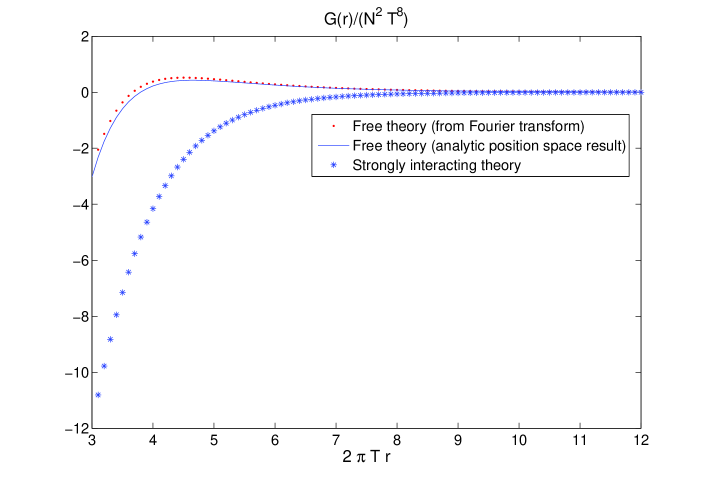
Figure 8: SYM correlators obtained by Fourier transform of the spectral function.

As a check on the numerical Fourier transforms themselves, we compute the corresponding Fourier transform in the free theory at finite temperature starting from the analytic expression for the spectral density Eq. (10); in this case an analytic expression also exists directly in position space, Eq. (8), providing a non-trivial check on the accuracy of the Fourier transform. In both cases we subtract the zero-temperature contribution, which, as mentioned above, is independent of the coupling. The step sizes in $\bar{\omega}$ and $\bar{k}$ are both 0.1, and the chosen range of integration is 0 to 20. The result of this numerical integration is shown in Fig. 8, where we have fixed $\tau=\frac{1}{2\pi T}$. With $x$ ranging over values much larger than $\tau$, the Figure shows the departure of the Fourier-transformed correlator from the direct evaluation of the $x$-space expression (8). The achieved accuracy is sufficient for our purposes. The largest discrepancy occurs at short distances, where the sensitivity to the discretization step and the finite range of $\omega$ is greatest.

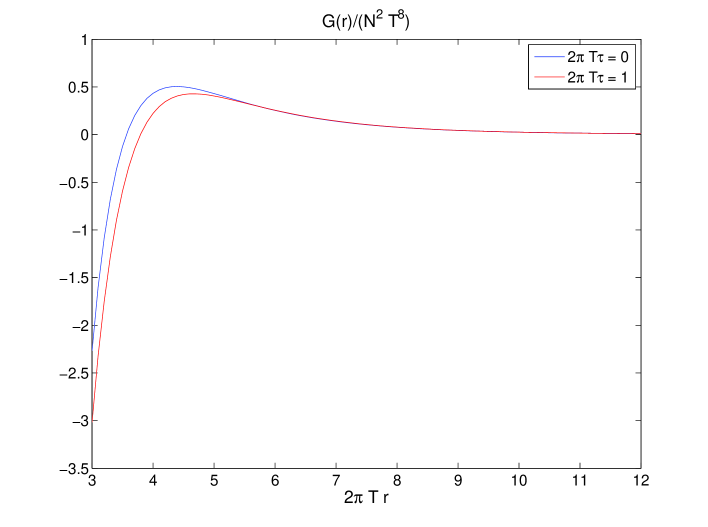
Figure 9: The free correlators with $2\pi T\tau=1$ and 0, Eq. (8).

To illustrate the dependence on the regulator $\tau$, we compare the correlator $C_{{{\mathcal{O}}}{{\mathcal{O}}}}(r,\tau,T)-C_{{{\mathcal{O}}}{{\mathcal{O}}}}(r,\tau,0)$ for $\tau=1/2\pi T$ with $G_{{{\mathcal{O}}}{{\mathcal{O}}}}(r,T)$ in the free case (Fig. 9). We see that for $r>5/2\pi T$, the correlators coincide to the accuracy needed for our purposes.

4 Correlators on the lattice

In this section we describe the lattice setup and the numerical results obtained by Monte-Carlo simulations. We employ the Wilson action [40],

$$S_{\rm g}=\frac{1}{g_{0}^{2}}\sum_{x,\mu\neq\nu}{\rm tr}\{1-P_{\mu\nu}(x)\}\,,$$ (22)

where the ‘plaquette’ $P_{\mu\nu}$ is the product of four link variables $U_{\mu}(x)$ around an elementary cell in the $(\mu,\nu)$ plane.

As a simulation algorithm, we use the standard combination of heatbath and over-relaxation [41, 42, 43, 44] sweeps for the update in a ratio increasing from 3 to 5 as the lattice spacing is decreased. The overall number of sweeps between measurements was typically between 4 to 12.

4.1 Discretization and normalization of the operators

A choice has to be made for the discretization of the operators $\theta(x)$ and $q(x)$. Here we use the specific discretization

$$\theta_{L}(x) \equiv -\chi_{s}(g_{0})\frac{dg_{0}^{-2}}{d\log a}~{}\frac{1}{2}\sum_{\mu,\nu}\mathop{\rm Re}{\rm tr}\Big{[}\widehat{F}_{\mu\nu}(x)\widehat{F}_{\mu\nu}(x)\Big{]}\,,$$ (23)

$$q_{L}(x) \equiv \frac{-Z_{q}(g_{0})}{32\pi^{2}}\epsilon_{\mu\nu\rho\sigma}{\rm tr}\Big{[}\widehat{F}_{\mu\nu}(x)\widehat{F}_{\rho\sigma}(x)\Big{]}\,,$$ (24)

where the (antihermitian) ‘clover’ discretization of the field-strength tensor $\widehat{F}_{\mu\nu}(x)$ is defined in terms of the link variables in [45]. In this work we feed in ‘HYP smeared’ link variables [46] into the definition of $\widehat{F}_{\mu\nu}(x)$. The name stems from the fact that the elementary link variable is replaced by an average of Wilson lines which remain in the adjacent elementary hypercubes. We kept the original parameters [46] and used the projection onto the SU(3) group of the Wilson-line average described in [47].

At the quantum level, the normalization of these lattice operators differs from the naive normalization. Indeed, even though the anomalous dimension of these operators vanishes, a finite renormalization of the operators survives, which has to be compensated for in order to ensure that their on-shell matrix elements approach their continuum limit with O($a^{2}$) corrections.

In Eq. (23), $\frac{dg_{0}^{-2}}{d\log a}$ is the lattice beta-function which describes by how much the lattice spacing shrinks when the bare coupling is reduced. While asymptotically it is governed by the first two universal beta-function coefficients, we work in the region $g_{0}^{2}\sim 1$ and therefore employ a non-perturbatively determined beta-function. Specifically we use the quantity $r_{0}/a$ (the Sommer reference scale) as a function of $g_{0}^{2}$, as computed in [48] and parametrized in the appendix of [49]. By taking one derivative of the parametrization, we obtain $\frac{dg_{0}^{-2}}{d\log a}$.

The trace anomaly in our chosen discretization still requires the additional normalization factor $\chi_{s}(g_{0})$. The latter is fixed by calibrating against the ‘canonical’ discretization of $\theta(x)$. This discretization $\theta_{L}^{\prime}$ arises from differentiating the lattice action (22) with respect to the bare coupling,

$$a^{4}\theta_{L}^{\prime}(x)=\frac{dg_{0}^{-2}}{d\log a}\sum_{\mu,\nu}\mathop{\rm Re}{\rm tr}\Big{[}1-P_{\mu\nu}(x)\Big{]}.$$ (25)

By requiring that $e-3p$ be independent of the discretization, i.e. $\langle\theta_{L}(x)\rangle_{T}-\langle\theta_{L}(x)\rangle_{0}$ be equal to $\langle\theta_{L}^{\prime}(x)\rangle_{T}-\langle\theta_{L}^{\prime}(x)\rangle_{0}$, we determine $\chi_{s}(g_{0})$. Here we choose $N_{\tau}\equiv L_{0}/a=6$ to do this matching. The results are well parametrized by

$$\chi_{s}(g_{0})=\frac{0.3257}{1-0.7659g_{0}^{2}},\quad 5.90\leq\beta\leq 6.72.$$ (26)

The error varies from 0.004 at $\beta=6.0$ to 0.008 at $\beta=6.72$. We have not investigated systematically the dependence of $\chi_{s}$ on the value of $N_{\tau}$ used for the matching. This uncertainty is not included in the above error estimates, and requires repeating the matching calculation at $N_{\tau}=8$ or $12$. For our purposes in this work, this uncertainty will not prevent us from drawing conclusions when comparing the trace anomaly correlator to theoretical predictions.

4.1.1 Normalization of the topological charge density

The procedure we use to normalize $q_{L}(x)$ is somewhat new to our knowledge, and therefore we describe it in some detail. We again exploit the fact that there exists a discretization $q_{L}^{\prime}(x)$ for which the normalization is known exactly. This is the definition based on the overlap operator [50] which satisfies the Ginsparg-Wilson relation [51]. Indeed, $Q_{L}^{\prime}(x)=\sum_{x}q_{L}^{\prime}(x)$ is then guaranteed to be an integer on every gauge field configuration, because it counts the difference of the number of right-handed and left-handed zero-modes of the Dirac operator [52].

We normalize our discretization of $q(x)$ by matching the value of its vacuum two-point function with the same correlator obtained with the overlap-fermion-based discretization of $q(x)$. The latter correlator was obtained in [53], and we use the numerical data of that article to fix the normalization of our discretization. More precisely, the quantity matched is $r^{8}\,C_{qq}(r,0)$; this removes the largest part of the uncertainty in the lattice spacing in physical units.

Specifically, we choose the matching distance to be $\bar{r}/r_{0}\simeq 0.68$, and use the data of [53] on the finest lattice (${\cal E}_{3}$ ensemble at $a=0.082$fm). The matching distance $\bar{r}$ was chosen such that on this lattice, $\bar{r}/a=3\sqrt{2}$. The lattice spacing in [53] is specified by the string tension, and we have used the factor $r_{0}\sqrt{\sigma}=1.1611(95)$ (based on the compilation [25]) to convert physical distances in units of $r_{0}$.

Given our normalization strategy, it is convenient to split the normalization factor of the operator into two parts:

$$Z_{q}(\beta)=Z_{q}(\beta_{\rm ref})\cdot\chi(\beta).$$ (27)

where we choose $\beta_{\rm ref}=6.2822$. The advantage of this separation is that only $Z_{q}(\beta_{\rm ref})$ depends on the overlap-based correlator. The latter has been calculated to much lower statistics than our computationally cheaper correlator. We find

$$Z_{q}(\beta_{\rm ref})=1.55(8)\,,$$ (28)

where the uncertainty comes almost entirely from the overlap data. We then obtain, by matching the correlator at other values of $\beta$,

$$\chi(5.903) = 1.25(4)\qquad r_{\rm match}/r_{0}=0.94$$ (29)

$$\chi(6.018) = 1.125(24)\qquad r_{\rm match}/r_{0}=0.77$$ (30)

$$\chi(6.200) = 1.030(15)\qquad r_{\rm match}/r_{0}=0.68$$ (31)

$$\chi(6.408) = 0.959(20).\qquad r_{\rm match}/r_{0}=0.60\,$$ (32)

$$\chi(6.720) = 0.958(50).\qquad r_{\rm match}/r_{0}=0.60\,.$$ (33)

When necessary, we use linear interpolations in $r$ of the function $r^{8}\,C_{qq}(r,0)$ to match different lattice spacings. These $\chi$ factors are well parametrized as

$$\chi(\beta)=\frac{0.8112-0.7388g_{0}^{2}}{1-0.9364g_{0}^{2}},\qquad\beta=6/g_{0}^{2}\,.$$ (34)

The absolute error is about 0.041 at $\beta=5.9$, 0.014 at $\beta=6.1$, 0.010 at $\beta=6.4$ and 0.026 at $\beta=6.7$.

4.2 The vacuum correlators ($T=0$)

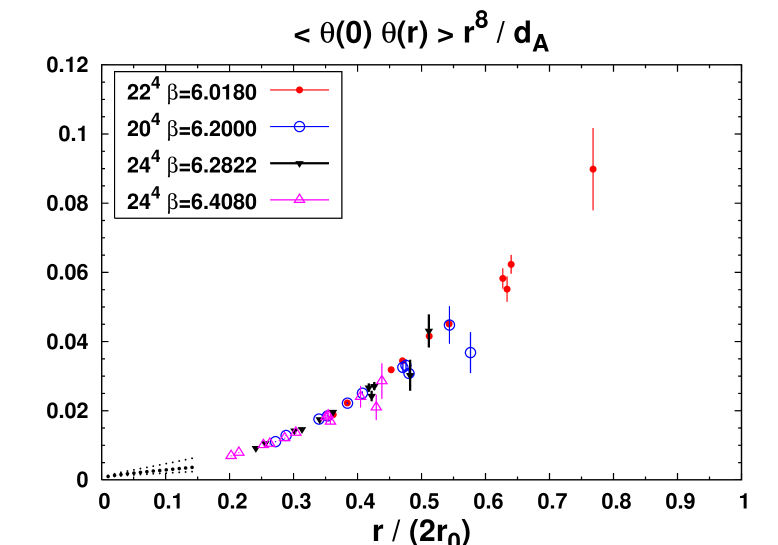
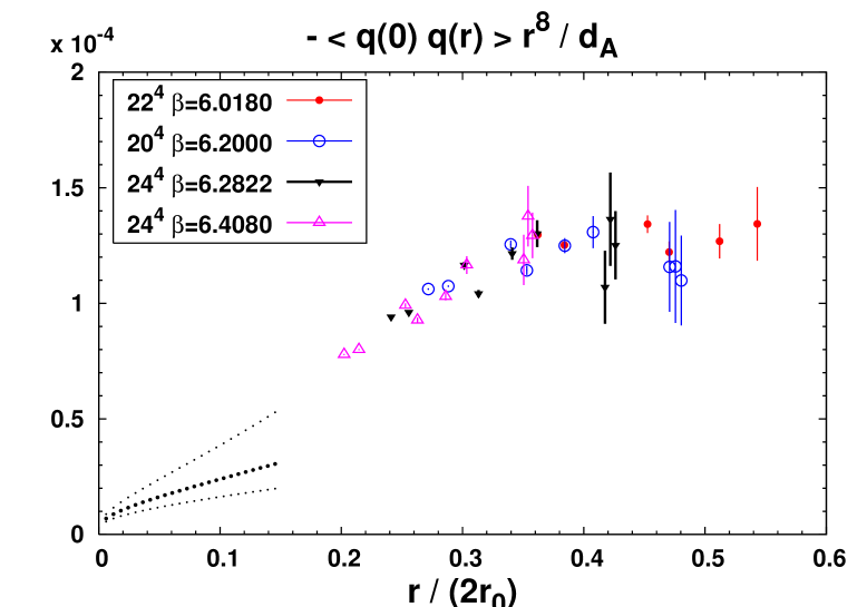
Figure 1: Zero-temperature correlator of the trace anomaly $\theta(x)$ (top) and of the topological charge density $q(x)$ (bottom). The overall normalization in the latter case is fixed by the data of Horvath et al. [53]. The dotted lines at small $r$ correspond to the one-loop result with choices of renormalization scale (from top to bottom) $\mu=\frac{\pi}{2r},\frac{\pi}{r}$ and $\frac{2\pi}{r}$.

The vacuum correlators of the trace anomaly and the topological charge density (multiplied by $r^{8}$) are displayed in Fig. 1. The overall normalization uncertainty coming from $\chi_{s}(g_{0})$ and $Z_{q}(\beta)$ are not included in the error bars on the picture; they are given above. Only data points with $r/a\geq 4$ are displayed. We have measured the correlator along the lattice axes (1,0,0), (1,1,0) and (1,1,1) and averaged the results over all equivalent directions. Some of the raw data is given in Tables (1) and (2).

The plots also show the perturbative prediction (7) at small distances. The three lines give an indication of the renormalization scale uncertainty: they correspond to $\mu=\frac{\pi}{2r},\frac{\pi}{r},\frac{2\pi}{r}$. For that purpose we have used the result $\Lambda^{(N_{\rm f}=0)}_{\overline{\rm MS}}r_{0}=0.602(48)$ [54]. Based on these figures, it is very plausible that our data agrees with perturbation theory at short distances, but data at smaller lattice spacing is needed for a more stringent test.

Such vacuum correlators are of course interesting in their own right. In particular, they can be used to test models for low-energy QCD, such as the instanton-liquid model [55] or the more recent holographic models of hadrons [56]. See [57, 58] for model calculations of gluonic vacuum correlators. A detailed comparison of the latter with lattice data will be carried out elsewhere; for the time being we simply note that around $r=0.4$fm the lattice data points lie on a convex curve in the scalar case, and a concave curve in the pseudoscalar case. This observation is qualitatively consistent with the instanton-model calculations of [57], where it is interpreted as an attraction/ repulsion respectively in the scalar and pseudoscalar channels.

4.3 Finite-temperature correlators

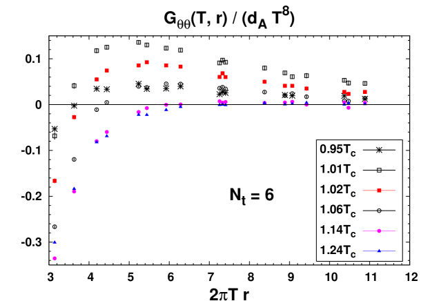
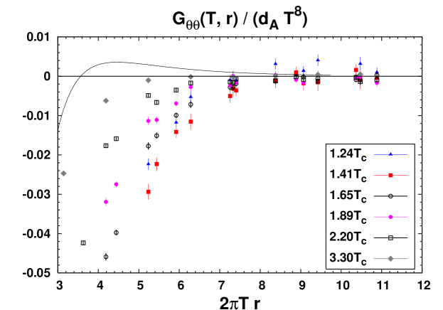
Figure 2: Thermal part of the spatial correlator of the trace anomaly $\theta$, at $N_{\tau}=6$ and several temperatures. The curve in the lower panel is the one-loop result (Eq. 7) with choice of renormalization scale described in section (4.3).

The finite-temperature correlators of the trace anomaly minus their zero-temperature counterpart are displayed in Fig. (2). Partial results for this quantity were already published in [23]. A sample of the raw data is presented in Tables (3) and (4).

Starting from the higher temperatures (bottom panel), we note that the lattice correlators are gradually approaching the free-theory prediction (Eq. 7) as the temperature is raised, as one expects on the basis of asymptotic freedom. In order to display Eq. (7) on the figure, we have set the renormalization scale to $\mu=\pi(T+\frac{1}{r})$ and used $\Lambda^{(N_{\rm f}=0)}_{\overline{\rm MS}}r_{0}=0.602(48)$ [54]. However, at the temperatures where simulation data are available, the subtracted correlator is negative at all separations $r$ – unlike the free correlator. This means that the plasma screens the fluctuations of the operator $\theta$ more than the vacuum does.

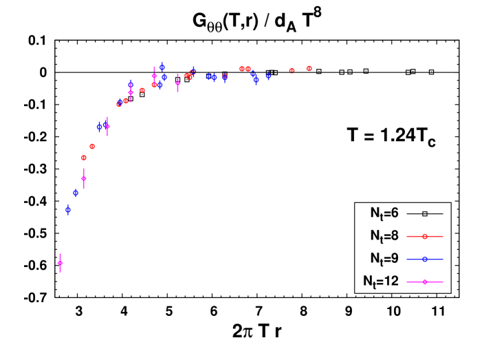
Figure 5: Thermal part of the spatial correlator of the trace anomaly (top) and topological charge density (bottom), at $T=1.24T_{c}$. The curve in the lower panel is the one-loop result (Eq. 7) with the same choice of renormalization scale as in Fig. (2).

We have checked for discretization errors by calculating $G_{\theta\theta}(r,1.24T_{c})$ at several lattice spacings. This means that $N_{\tau}=(aT)^{-1}$ is varied and $\beta$ tuned so that the temperature is kept fixed. The result is shown in Fig. (5), top panel. To a good approximation, the data fall on a single curve. It is not presently our intention to carry out a systematic continuum extrapolation of $G_{\theta\theta}(r,T)$ in $1/N_{\tau}^{2}$. Rather we want to show convincing evidence that the conclusions we draw from finite lattice spacing data are not affected by discretization errors.

In the figures, we have not included the statistical uncertainty on the non-perturbative normalization factors. However the latter cancel in the ratio

$$\frac{G_{\theta\theta}(r,T)}{(e-3p)^{2}}\,,$$ (35)

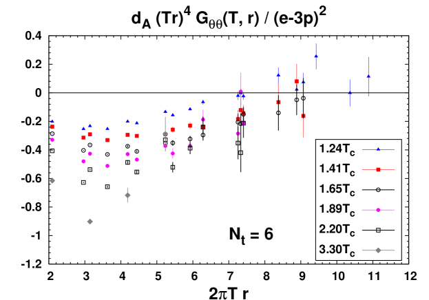
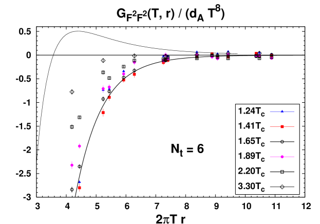
Figure 3: Top: thermal part of the spatial correlator of the trace anomaly $\theta$, normalized by $(e-3p)^{2}$ (which cancels the renormalization factor). Bottom: comparison of the $F^{2}$ correlator in the 3-loop $\overline{\rm MS}$ scheme to the one-loop result (upper curve) and the SYM correlator (lower curve).

which is displayed in Fig. 3, top panel. We have multiplied this quantity by $d_{A}$ so as to give it a finite limit when $N_{c}\to\infty$ and by $(Tr)^{4}$, so that the expected short-distance behavior is $\sim\alpha_{s}^{2}(\mu)$, where $\mu={\rm O}(1/r)$. The graph shows that $G_{\theta\theta}(r,T)$ falls off like $1/r^{4}$, as expected from the OPE, for $3<2\pi Tr<5$. Beyond this interval, it falls off faster to zero.

The on-shell correlation functions of $\theta$ are renormalization-group invariant. However, if we want to compare the result with the ${\cal N}=4$ SYM correlator of $F^{2}$ described in section (3), we have to divide out the factor of $\beta(g)/2g$ that multiplies the Yang-Mills operator $\theta$. Since the beta-function is scheme-dependent, this means that the renormalized $F^{2}$ correlator in the Yang-Mills theory is scheme-dependent, too. We choose the three-loop $\overline{\rm MS}$ scheme, and evaluate the coupling $\alpha_{s}$ at the scale $\mu(r,T)=\frac{3}{8}\pi(T+1/r)$. A few remarks may be useful to motivate this choice. At $r=1/T$, this corresponds to $\mu=\frac{3\pi}{4r}$; it makes the one-loop prediction for the $\theta$ correlator approximately go through the lattice data at $T=0$, see Fig. (1). At short distances, we expect $r$ to provide the harder scale and therefore the appropriate $\mu$ to be dominated by $r$. For $r>T$, we expect the momenta of the two exchanged gluons to be of order $\pi T$. The chosen expression for $\mu$ is then a simple interpolation between these two regimes.

We thus obtain the lattice data for the $F^{2}$ correlator in the $\overline{\rm MS}$ scheme, see the bottom panel of Fig. 3. We are then in a position to carry out a parameter-free comparison with the one-loop result Eq. (7) and the AdS/CFT result. In the range of temperatures $1.2<T/T_{c}<1.9$, the lattice correlators are in semi-quantitative agreement with the corresponding $F^{2}$ correlator calculated in the strongly coupled ${\cal N}=4$ SYM theory. The lattice data are negative at all $1/2T<r<1/T$, and this is in contrast with the free-field theory result, which is positive in that range. The data at $T>2T_{c}$ however does suggest that the non-perturbative correlator gradually moves towards the one-loop result as the temperature increases, as expected from asymptotic freedom.

Coming back to Fig. 2 (top panel), the thermal fluctuations become stronger as the temperature is lowered toward $T_{c}$, to the point where the subtracted correlator is positive over a wide range of distances $r$. Unsurprisingly this fact is accounted for neither by the weak coupling predictions, nor by the conformal ${\cal N}=4$ SYM result. The correlation between the fluctuations of $\theta$ is strongest at $1.01T_{c}$, and drops again as one moves away from the transition below $T_{c}$. The interpretation of the data is helped by the fact that the overall fluctuations of $\theta$ are related to thermodynamic properties via the sum rule [59, 60]

$$\int d^{4}x\,\langle\theta(x)\theta(0)\rangle_{{\rm conn},T-0}=T^{5}\frac{\partial}{\partial T}\frac{e-3p}{T^{4}}.$$ (36)

Since we know that $(e-3p)/T^{4}$ rises very steeply between $T_{c}$ and $1.1T_{c}$ [61], Eq. (36) indicates that the fluctuations of $\int d^{4}x\,\theta$ are strongest in that range of temperatures. Since the Wilson coefficients in the OPE are negative, there is a negative contribution to the LHS of Eq. (36) from the short-distance part of the correlator. Therefore there has to be an enhancement in the $\theta$ two-point function at intermediate or long distances in order to account for the positive sign of the RHS (note however that here we restrict ourselves to equal-time correlators). On the other hand, above $1.13T_{c}$, where the RHS of Eq. (36) is negative, there is no necessity for $G_{\theta\theta}$ to be positive at any non-vanishing separation. Our data shows that indeed $G_{\theta\theta}$ at intermediate distances $r\approx 1/T$ is negative for all available temperatures above $1.2T_{c}$. This differs from the correlator $G_{ee}$ of the energy density [23], which is positive at intermediate separations.

4.3.1 Topological charge density correlator

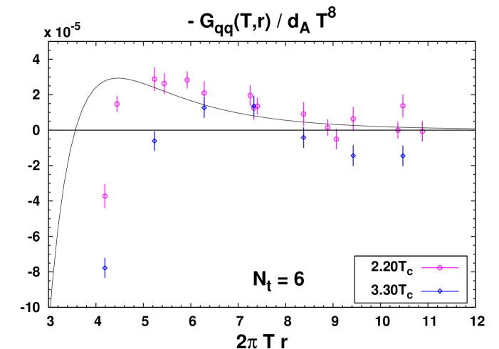
Figure 6: Detail of the thermal part of the spatial correlator of the topological charge density $q(x)$ at $\beta=6.408$, compared to the one-loop result (Eq. 7) with the same choice of renormalization scale as in Fig. (2).

We now discuss the topological charge density correlator, starting from the high temperature end. An example of $G_{qq}$ at high-temperatures is displayed in Fig. (6). We see that qualitatively, the correlator, in the interval where data is available, resembles its free-theory counterpart: $-G_{qq}$ is negative at short-distance, as predicted by the OPE, and then positive at intermediate distances. On the basis of the pseudoscalar screening masses, we expect $G_{qq}$ to approach zero from below, and there is a hint at $3.30T_{c}$ that indeed it does.

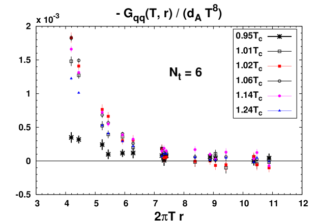
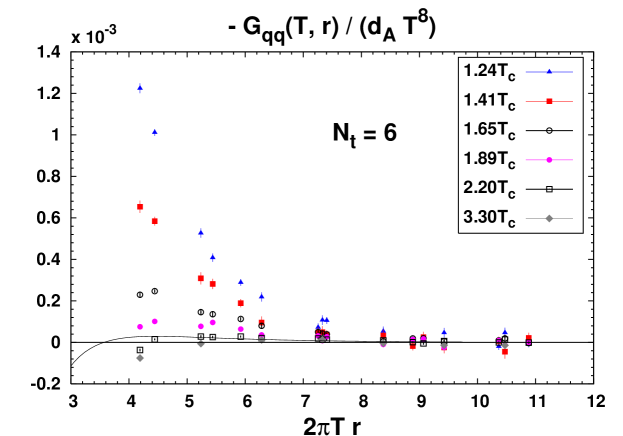
Figure 4: Thermal part of the spatial correlator of the topological charge density $q$, at $N_{\tau}=6$ and several temperatures. The curve in the lower panel is the one-loop result (Eq. 7) with the same choice of renormalization scale as in Fig. (2).

If we now lower the temperature, as shown in Fig. (4, bottom panel), we see that the range of distances where $-G_{qq}$ is positive grows, and that its maximum value also grows. The OPE tells us that at sufficiently short distances, $-G_{qq}$ must be negative. Below $1.6T_{c}$ its maximum is no longer visible in the data; we conjecture that it is located at too short distance $r$ for us to see it in the lattice data (at short distances, we are limited by discretization errors).

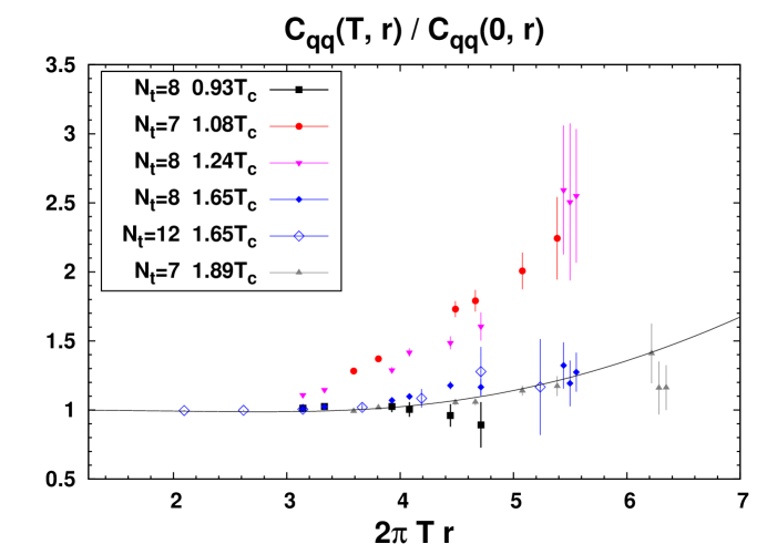
Figure 7: Ratio of the finite-temperature spatial correlator of the topological charge density $q(x)$ to the zero-temperature one. The curve is the one-loop result (Eq. 7).

As we lower the temperature further (top panel of Fig. (4)), $-G_{qq}(r,T)$ at fixed $r$ continues to grow. It hits a maximum between $1.02$ and $1.06T_{c}$. Thus similarly to the trace anomaly, the topological charge density exhibits strong spatial correlations near $T_{c}$. How strong they are is better illustrated by taking the ratio of the finite-temperature to the zero-temperature data, Fig. (7). Here one clearly sees that for $r$ of order $1/T$, the spatial correlation of topological charge density fluctuations is about twice as strong near $T_{c}$ as in the vacuum. A technical advantage of this ratio is that the overall normalization cancels out, and secondly that we expect a partial cancellation of the discretization errors to take place.

To check that these large correlations are not a cutoff effect – there is after all a large cancellation taking place at short distance in the subtracted correlator – we have repeated the $1.24T_{c}$ calculation at a finer lattice spacing. The comparison is shown in Fig. (5). We see that the different data sets fall on top of eachother within errors in the interval $0.4<Tr<1.2$. We thus conclude that the strong, finite-temperature induced enhancement of the correlation is a true physical effect.

There are significant differences between the scalar and the pseudoscalar channels in the lattice data at distances $1/2T<r<T$. This is unlike the strongly coupled ${\cal N}=4$ SYM theory, where the $F^{2}$ and $F\tilde{F}$ correlators are identical. It is also unlike the free field prediction. In the OPE framework, this difference requires operators of dimension 6 or higher to overwhelm the expectation value of the stress-energy tensor in Eq. (9). This would in turn imply the breakdown of the OPE as an asymptotic expansion.

Our discovery of large spatial correlations in the topological charge density fluctuations in the vicinity of $T_{c}$ is qualitatively in agreement with the results of [62]. The latter showed a strong suppression of the topological susceptibility just above $T_{c}$, using a method based on the semi-classical identification of topological charges. This suppression is particularly dramatic at larger $N_{c}$ values, but even for SU(3) it amounts to a factor of about 0.54(4). This implies that $-\int d^{4}x\langle q(x)q(0)\rangle_{T-0}\geq 0$, and therefore there has to be a range of separations $x$ where $-\langle q(x)q(0)\rangle_{T-0}$ is positive; this is what we are seeing in the data. Note that the short-distance singularity of $\langle q(x)q(0)\rangle_{T-0}\propto\alpha_{s}^{2}/x^{4}$ gives a finite contribution when integrated over space-time. This is in contrast with the topological susceptibility itself, $\chi_{t}\equiv\int d^{4}x\langle q(x)q(0)\rangle_{0}$, which has to be defined with care [63] if it is to remain finite when the cutoff is removed.

5 The effective coupling in the plasma

We have found that the strongly coupled SYM theory has an $F^{2}$ correlator similar to the pure Yang-Mills theory in the deconfined phase below $2T_{c}$. To summarize the procedure, we have calculated the $\theta$ correlator on the lattice, which contains a factor $(\beta(g)/2g)^{2}$ relative to the $F^{2}$ correlator. This factor makes it renormalization-group invariant in the pure Yang-Mills theory. We used the 3-loop $\overline{\rm MS}$ scheme for the beta-function to convert the lattice $\theta$ correlator to the $F^{2}$ correlator, and found semi-quantitative agreement between the theories in a range of temperatures. For $r=1/T$, the values for our chosen running coupling are

$$\alpha_{s}(T)=0.33,~{}~{}0.30,~{}~{}0.27,~{}~{}0.25,~{}~{}0.23,~{}~{}0.19$$ (37)

for the six temperatures displayed on the bottom panel of Fig. (2). From Fig. (3), we see that at the last two temperatures, the Yang-Mills $F^{2}$ correlator no longer agrees with the strongly coupled SYM result. Therefore we conclude that for $\alpha_{s}$ smaller than about $0.25$ (i.e. $\lambda$ smaller than about 10), one should not expect other properties of the Yang-Mills plasma to coincide with those of the infinite-coupling SYM plasma. In fact it is somewhat surprising that for $0.25<\alpha_{s}<0.30$, where the function $\alpha_{\overline{\rm MS}}(\mu)$ shows a modest dependence on the order in perturbation theory, the thermal correlator is so much more similar to the strongly coupled SYM correlator than to the weakly coupled one. This may be related to the fact that at finite temperature, due to infrared effects, the perturbative expansion parameter is $g$ rather than $\alpha_{s}$. Thus at an energy scale where the vacuum polarization effects are still well approximated by the perturbative expansion, the thermal physics rather has a strong coupling character.

We now discuss whether one may use the ‘empirically’ observed similarity to match the couplings of the Yang-Mills and SYM theories. By ‘matching’, we mean to find a way of comparing the two theories in such a way that they share as many properties as possible at a semi-quantitative level . Since the ’t Hooft coupling is the unique parameter of the SYM theory, this is the only parameter we need to fix in the comparison. To what extent several observables can be simultaneously made similar provides a clue as to how universal the properties of non-Abelian plasmas are.

The best way to match QCD with a different theory is presumably to equate a renormalized quantity such as the Debye mass [21] across the two theories. However this requires knowing the relation between the coupling and the Debye mass on the SYM side. A technical obstacle to this program is that the Debye mass is independent of the coupling in the limit of large coupling. Other observables typically lead to the same lack of sensitivity to $\lambda$. One then needs to know $1/\lambda$ corrections to the selected observable on the SYM side, which leads to more involved calculations and raises questions of convergence, etc.

A different way to match the two theories is to define a running coupling based on a renormalized quantity, such that the weak-coupling relation holds by definition for all scales. One then equates the couplings of the two theories. For example, one can define a Yang-Mills effective coupling from the Debye mass, $\lambda(T)\equiv 3\frac{m_{D}^{2}}{T^{2}}$ in the SU($N_{c}$) gauge theory, and use that value of $\lambda$ in the SYM theory. A priori, when the coupling is large, its scheme dependence is strong. For this reason, we expect that matching the observable itself is the superior procedure.

Nevertheless the non-trivial agreement of the Yang-Mills and the SYM $F^{2}$-correlators in a range of temperatures suggests that simply using the values of $\lambda=12\pi\alpha_{s}=10\dots 12$, where the temperature-dependent values of $\alpha_{s}$ are given in Eq. (37), is a reasonable choice of coupling constant to use on the SYM side. This is a moderately large coupling constant; for instance, the O($1/\lambda^{3/2}$) correction to the $\lambda=\infty$ shear viscosity to entropy density ratio $\eta/s$ is about $+50\%$ at this coupling [64, 65, 66].

6 Summary

We have found that the gluon plasma generically screens scalar and pseudoscalar fluctuations more than the vacuum does at short distance $r\ll 1/T$ and at long distances $r\gg 1/T$. Near $T_{c}$ however, there is a significant range of distances of order $1/T$ over which the spatial correlations are stronger in the plasma than in the vacuum. We interpret this fact as there being stronger fluctuations of wavelength O($1/T$) in the plasma than in the vacuum. As one increases the temperature above $T_{c}$, this effect disappears soon in the scalar channel, but extends to about $2T_{c}$ in the pseudoscalar case. In the latter channel, the enhancement of these fluctuations over those of the vacuum is about a factor two. While the pseudoscalar and scalar channels are expected to have similar correlation functions at very short distances and they precisely agree in the SYM theory, the two channels look rather different at least up to $2T_{c}$, according to our lattice data. The scalar correlator agrees well with the corresponding correlator in the strongly coupled SYM theory in the range of temperatures $1.2<T/T_{c}<1.9$, while the pseudoscalar correlator is notably different due to the aforementioned strong fluctuations. These observations constitute our main results. The scalar fluctuations of wavelength $\sim 1/T$ are suppressed compared to the vacuum, while the pseudoscalar fluctuations are significantly enhanced. It would be interesting to see whether a next-to-leading order perturbative calculation would agree significantly better with the lattice data than the treelevel calculation does.

We note that studying the vacuum subtracted correlators of gauge invariant operators at distances short compared to $1/T$ is morally equivalent, via the operator-product expansion, to investigating the thermal expectation values of higher-dimensional renormalized operators. Our study thus has goals in common with the investigation of twist-two operator expectation values [13].

The semi-quantitative agreement of the scalar correlators between the pure Yang-Mills and the SYM theories, while the pseudoscalar channel is markedly different, highlights the fact that different plasmas can exhibit quite similar properties in some channels while differing substantially in others.

In spite of having a reduced topological susceptibility [62], the deconfined phase close to $T_{c}$ exhibits strong correlations of $\vec{E}\cdot\vec{B}$ over distances of order $1/T$, which are stronger than in the vacuum by about a factor two. It would be interesting to see whether models of QCD can account for this effect. It would also be worth investigating how much this effect depends on the weakness of the first-order deconfining phase transition, and whether the effect persists at larger values of $N_{c}$, where the transition is strongly first order [67, 68]. A plausible mechanism for the observed strong spatial correlations is that fluctuations of $\vec{E}\cdot\vec{B}$ with a coherence length of at least $1/T$ occur in the plasma. Perhaps these fluctuations have been seen in [62], where the topological lump size was found to be peaked at $\rho\simeq 1.7/T_{c}$. This large size led the authors to conclude that this peak lies outside the range of applicability of their semiclassical methods. It is worth thinking about possible phenomenological implications of these large-amplitude, long-wavelength fluctuations, since the charge-separation effects of a non-zero $\vec{E}\cdot\vec{B}$ field configuration in the context of heavy ion collisions have recently received a lot of attention [69, 70, 71].

Appendix A Details of Numerical Integration

We must numerically integrate the flow equation (19)

$$\partial_{r}\tilde{\chi}=\frac{2i\bar{\omega}}{r^{2}\left(1-\frac{1}{r^{4}}\right)}\left[{\tilde{\chi}^{2}\over r^{3}}-r^{3}\left[1-\frac{\bar{k}^{2}}{\bar{\omega}^{2}}\left(1-\frac{1}{r^{4}}\right)\right]\right].$$ (38)

from the horizon at $r=1$ up to the AdS boundary at $r\to\infty$, which the initial condition $\tilde{\chi}(r=1)=1$. In practice we integrate to $r=20000$ and verify that further increasing the integration domain does not change the answer. Note that while $\mathop{\rm Im}(\chi)$ contains a divergence as $r\to\infty$, this is a standard UV divergence that contributes only a contact term, and can be removed by holographic renormalization. It will not concern us, as the real part of $\chi$ (and thus the imaginary part of $G_{R}$) has a finite limit as $r\to\infty$.

We cannot begin our integration at precisely $r=1$ as the equation is singular there. We thus build a series expansion of $\tilde{\chi}$ about $r=1$:

$$\tilde{\chi}=1+\tilde{\chi}_{1}(r-1)+\tilde{\chi_{2}}(r-1)^{2}+...$$ (39)

Plugging this into Eq. (38) we can determine the expansion coefficients $\chi_{n}$ up to any desired order. The expressions are lengthy but straightforward to obtain and so we do not present them here; however we use the first three terms in this expansion to find the value of $\tilde{\chi}(r=1+\delta)$ and use this the initial condition to begin our integration at a small finite value of $\delta$ ($\delta=0.01$ in practice).

Note also that if we keep $\bar{k}$ finite and take $\bar{\omega}\to 0$, the flow equation appears singular. However we know that at vanishing chemical potential the spectral density of a bosonic operator must be an odd function of $\bar{\omega}$, and thus vanishes as $\bar{\omega}\to 0$, although the precise point $\bar{\omega}=0$ presents numerical difficulties. Thus our code simply sets $\mathop{\rm Im}(G_{R}(\bar{\omega}=0))=0$ by hand.

	$22^{4},\,\beta=6.018$, $\frac{dg_{0}^{-2}}{d\log a}=-0.09922$		$24^{4},\,\beta=6.2822$, $\frac{dg_{0}^{-2}}{d\log a}=-0.1166$
$r/a$	$\chi_{s}=1.371$, $Z_{q}=1.742$		$\chi_{s}=1.220$, $Z_{q}=1.546$
	$r^{8}C^{\rm bare}_{\theta\theta}/d_{A}$	$-10^{4}\cdot r^{8}C^{\rm bare}_{qq}/d_{A}$	$r^{8}C^{\rm bare}_{\theta\theta}/d_{A}$	$-10^{4}\cdot r^{8}C^{\rm bare}_{qq}/d_{A}$
2.0000	0.00156574(33)	-0.043481(18)	0.00085488(12)	-0.0224117(68)
3.0000	0.0074804(48)	0.13816(24)	0.0037726(20)	0.12537(10)
4.0000	0.018866(42)	0.4276(22)	0.009190(18)	0.39384(93)
5.0000	0.03185(24)	0.443(12)	0.01424(10)	0.4876(55)
6.0000	0.0451(10)	0.443(52)	0.01965(43)	0.544(24)
7.0000	0.0552(37)	0.46(19)	0.0242(15)	0.571(84)
8.0000	0.056(10)	-0.17(55)	0.0303(44)	0.56(24)
9.0000	0.024(27)	-3.2(14)	0.038(11)	1.13(61)
10.0000	-0.045(72)	-9.0(35)	0.042(27)	3.5(14)
2.8284	0.0070641(29)	0.13736(13)	0.0038655(11)	0.124059(49)
4.2426	0.022254(50)	0.4127(25)	0.010561(22)	0.4021(11)
5.6569	0.04157(46)	0.418(25)	0.01751(20)	0.508(11)
7.0711	0.0623(27)	0.12(15)	0.0271(12)	0.523(62)
8.4853	0.090(12)	0.43(61)	0.0431(48)	0.64(28)
9.8995	0.122(41)	3.6(22)	0.044(17)	-0.36(94)
3.4641	0.013541(12)	0.33075(62)	0.0071350(55)	0.29340(29)
5.1962	0.03443(28)	0.403(15)	0.01465(12)	0.4360(66)
6.9282	0.0582(29)	0.40(15)	0.0267(12)	0.447(66)
8.6602	0.074(17)	0.69(88)	0.0357(72)	-0.04(37)
10.3923	0.057(74)	-2.6(39)	0.033(30)	0.7(17)

Table 1: Bare vacuum correlators for two different lattice spacings. See the main text for the origin of the normalization factors and their uncertainties.

	$20^{4},\,\beta=6.200$, $\frac{dg_{0}^{-2}}{d\log a}=-0.1120$		$24^{4},\,\beta=6.408$, $\frac{dg_{0}^{-2}}{d\log a}=-0.1226$
$r/a$	$\chi_{s}=1.262$, $Z_{q}=1.595$		$\chi_{s}=1.148$, $Z_{q}=1.495$
	$r^{8}C^{\rm bare}_{\theta\theta}/d_{A}$	$-10^{4}\cdot r^{8}C^{\rm bare}_{qq}/d_{A}$	$r^{8}C^{\rm bare}_{\theta\theta}/d_{A}$	$-10^{4}\cdot r^{8}C^{\rm bare}_{qq}/d_{A}$
2.0000	0.00100712(16)	-0.0263605(84)	0.000664435(84)	-0.0182749(46)
3.0000	0.0045234(23)	0.13444(12)	0.0028715(14)	0.110829(72)
4.0000	0.011065(21)	0.4172(11)	0.006926(13)	0.35415(70)
5.0000	0.01758(12)	0.4933(64)	0.010103(74)	0.4509(41)
6.0000	0.02506(53)	0.514(27)	0.01367(32)	0.530(17)
7.0000	0.0331(18)	0.456(96)	0.0187(11)	0.626(60)
8.0000	0.0448(54)	0.65(27)	0.0240(31)	0.75(18)
9.0000	0.081(16)	1.71(77)	0.0315(81)	1.15(46)
10.0000	0.191(44)	3.0(24)	0.038(19)	0.2(10)
2.8284	0.0045366(14)	0.132315(61)	0.00302558(77)	0.110874(35)
4.2426	0.012839(25)	0.4221(12)	0.007867(15)	0.36367(77)
5.6569	0.02218(23)	0.491(13)	0.01209(14)	0.4683(77)
7.0711	0.0308(13)	0.432(76)	0.01688(82)	0.588(45)
8.4853	0.0368(59)	-0.06(32)	0.0210(37)	0.93(20)
9.8995	0.067(21)	-0.7(11)	0.022(12)	1.72(68)
3.4641	0.0084346(62)	0.31326(31)	0.0055463(36)	0.26299(20)
5.1962	0.01849(14)	0.4490(77)	0.010459(86)	0.4218(49)
6.9282	0.0325(15)	0.455(76)	0.01813(86)	0.540(50)
8.6602	0.0336(85)	0.48(44)	0.0286(51)	1.07(29)
10.3923	0.010(37)	-0.0(19)	0.045(22)	0.4(12)

Table 2: Bare vacuum correlators for two different lattice spacings.

$r/a$	$6\times 28^{3}$		$9\times 28^{3}$
	$r^{8}C^{\rm bare}_{\theta\theta}/d_{A}$	$-10^{4}\cdot r^{8}C^{\rm bare}_{qq}/d_{A}$	$r^{8}C^{\rm bare}_{\theta\theta}/d_{A}$	$-10^{4}\cdot r^{8}C^{\rm bare}_{qq}/d_{A}$
2.0000	0.00079523(22)	-0.0194011(81)	0.00082743(11)	-0.0206983(56)
3.0000	0.0033813(42)	0.13059(20)	0.0035946(19)	0.132683(96)
4.0000	0.007945(38)	0.4061(20)	0.008540(18)	0.41965(93)
5.0000	0.01161(22)	0.563(12)	0.01270(10)	0.5784(56)
6.0000	0.01689(93)	0.696(52)	0.01814(45)	0.754(23)
7.0000	0.0245(33)	0.69(17)	0.0263(16)	0.960(80)
8.0000	0.0335(100)	0.17(53)	0.0312(46)	1.24(24)
9.0000	0.050(25)	-1.4(13)	0.022(12)	1.45(62)
10.0000	0.033(57)	0.5(31)	-0.012(28)	1.7(14)
2.8284	0.0035174(23)	0.128916(88)	0.0037160(11)	0.129810(44)
4.2426	0.008844(45)	0.4285(22)	0.009647(21)	0.4365(10)
5.6569	0.01319(43)	0.675(23)	0.01524(20)	0.655(11)
7.0711	0.0212(26)	0.94(14)	0.0249(12)	0.949(62)
8.4853	0.029(11)	1.59(56)	0.0356(52)	0.92(28)
9.8995	0.018(38)	1.9(19)	0.036(18)	1.76(92)
3.4641	0.006300(11)	0.30305(55)	0.0067527(53)	0.30710(26)
5.1962	0.01114(27)	0.563(14)	0.01264(12)	0.5582(66)
6.9282	0.0192(26)	0.86(14)	0.0219(12)	0.871(65)
8.6602	0.004(16)	1.30(85)	0.0243(73)	1.32(39)
10.3923	-0.104(72)	0.10(34)	0.000(30)	-1.2(17)

Table 3: Bare finite-temperature correlation functions at $\beta=6.2822$ ($\chi_{s}=1.220$, $Z_{q}=1.546$, $\frac{dg_{0}^{-2}}{d\log a}=-0.1166$).

$r/a$	$6\times 24^{3}$		$8\times 28^{3}$
	$r^{8}C^{\rm bare}_{\theta\theta}/d_{A}$	$-10^{4}\cdot r^{8}C^{\rm bare}_{qq}/d_{A}$	$r^{8}C^{\rm bare}_{\theta\theta}/d_{A}$	$-10^{4}\cdot r^{8}C^{\rm bare}_{qq}/d_{A}$
2.0000	0.000628574(92)	-0.0166504(39)	0.000644215(92)	-0.0171814(40)
3.0000	0.0026309(18)	0.110207(93)	0.0027312(17)	0.112619(90)
4.0000	0.006237(17)	0.34772(93)	0.006413(16)	0.35577(89)
5.0000	0.008967(97)	0.4805(55)	0.008905(92)	0.4822(54)
6.0000	0.01195(42)	0.623(24)	0.01185(41)	0.618(23)
7.0000	0.0131(15)	0.815(80)	0.0156(14)	0.747(76)
8.0000	0.0120(43)	1.15(24)	0.0217(40)	0.83(23)
9.0000	-0.001(11)	1.87(61)	0.028(10)	0.60(60)
10.0000	-0.042(25)	3.8(14)	0.014(25)	0.4(14)
2.8284	0.00280374(100)	0.111115(39)	0.00290514(97)	0.112818(40)
4.2426	0.006874(20)	0.36775(100)	0.007135(19)	0.3723(10)
5.6569	0.00990(19)	0.546(11)	0.00984(18)	0.5514(97)
7.0711	0.0139(12)	0.811(64)	0.0134(11)	0.749(61)
8.4853	0.0190(48)	1.03(27)	0.0183(46)	0.71(27)
9.8995	0.006(16)	1.71(92)	0.033(16)	0.06(90)
3.4641	0.0050233(48)	0.26228(25)	0.0052397(47)	0.26601(24)
5.1962	0.00836(12)	0.4586(65)	0.00886(11)	0.4630(63)
6.9282	0.0136(12)	0.814(65)	0.0130(11)	0.714(63)
8.6602	0.0133(68)	0.64(39)	0.0197(65)	0.61(37)
10.3923	-0.030(29)	0.1(17)	0.087(29)	-3.6(17)

Table 4: Bare finite-temperature correlation functions at $\beta=6.408$ ($\chi_{s}=1.148$, $Z_{q}=1.495$, $\frac{dg_{0}^{-2}}{d\log a}=-0.1226$).

References

- [1] B. Mueller, Theoretical challenges posed by the data from RHIC, Prog. Theor. Phys. Suppl. 174 (2008) 103–121.
- [2] PHENIX Collaboration, A. Adare et. al., Scaling properties of azimuthal anisotropy in Au + Au and Cu + Cu collisions at s(NN)**(1/2) = 200-GeV, Phys. Rev. Lett. 98 (2007) 162301, [nucl-ex/0608033].
- [3] H. B. Meyer, Transport properties of the quark-gluon plasma from lattice QCD, arXiv:0907.4095.
- [4] D. Teaney, Finite temperature spectral densities of momentum and R- charge correlators in N = 4 Yang Mills theory, Phys. Rev. D74 (2006) 045025, [hep-ph/0602044].
- [5] K. Kajantie, M. Laine, K. Rummukainen, and Y. Schroeder, The pressure of hot QCD up to g**6 ln(1/g), Phys. Rev. D67 (2003) 105008, [hep-ph/0211321].
- [6] A. Hietanen, K. Kajantie, M. Laine, K. Rummukainen, and Y. Schroeder, Three-dimensional physics and the pressure of hot QCD, Phys. Rev. D79 (2009) 045018, [arXiv:0811.4664].
- [7] J. P. Blaizot, E. Iancu, and A. Rebhan, On the apparent convergence of perturbative QCD at high temperature, Phys. Rev. D68 (2003) 025011, [hep-ph/0303045].
- [8] J.-P. Blaizot, E. Iancu, and A. Rebhan, Thermodynamics of the high-temperature quark gluon plasma, hep-ph/0303185.
- [9] S. S. Gubser, I. R. Klebanov, and A. W. Peet, Entropy and Temperature of Black 3-Branes, Phys. Rev. D54 (1996) 3915–3919, [hep-th/9602135].
- [10] M. Laine and Y. Schroeder, Two-loop QCD gauge coupling at high temperatures, JHEP 03 (2005) 067, [hep-ph/0503061].
- [11] J. Alanen, K. Kajantie, and V. Suur-Uski, Spatial string tension of finite temperature QCD matter in gauge/gravity duality, arXiv:0905.2032.
- [12] M. Cheng et. al., Baryon Number, Strangeness and Electric Charge Fluctuations in QCD at High Temperature, Phys. Rev. D79 (2009) 074505, [arXiv:0811.1006].
- [13] E. Iancu and A. H. Mueller, A lattice test of strong coupling behaviour in QCD at finite temperature, arXiv:0906.3175.
- [14] V. A. Novikov, M. A. Shifman, A. I. Vainshtein, and V. I. Zakharov, In a Search for Scalar Gluonium, Nucl. Phys. B165 (1980) 67.
- [15] V. A. Novikov, M. A. Shifman, A. I. Vainshtein, and V. I. Zakharov, Operator expansion in Quantum Chromodynamics beyond perturbation theory, Nucl. Phys. B174 (1980) 378.
- [16] J. M. Maldacena, The large N limit of superconformal field theories and supergravity, Adv. Theor. Math. Phys. 2 (1998) 231–252, [hep-th/9711200].
- [17] S. S. Gubser, I. R. Klebanov, and A. M. Polyakov, Gauge theory correlators from non-critical string theory, Phys. Lett. B428 (1998) 105–114, [hep-th/9802109].
- [18] E. Witten, Anti-de Sitter space, thermal phase transition, and confinement in gauge theories, Adv. Theor. Math. Phys. 2 (1998) 505–532, [hep-th/9803131].
- [19] P. Kovtun, D. T. Son, and A. O. Starinets, Viscosity in strongly interacting quantum field theories from black hole physics, Phys. Rev. Lett. 94 (2005) 111601, [hep-th/0405231].
- [20] H. Liu, K. Rajagopal, and U. A. Wiedemann, Calculating the jet quenching parameter from AdS/CFT, Phys. Rev. Lett. 97 (2006) 182301, [hep-ph/0605178].
- [21] D. Bak, A. Karch, and L. G. Yaffe, Debye screening in strongly coupled N=4 supersymmetric Yang-Mills plasma, JHEP 08 (2007) 049, [arXiv:0705.0994].
- [22] A. L. Kataev, N. V. Krasnikov, and A. A. Pivovarov, Two-loop calculations for the propagators of gluonic currents, Nucl. Phys. B198 (1982) 508–518, [hep-ph/9612326].
- [23] H. B. Meyer, Density, short-range order and the quark-gluon plasma, Phys. Rev. D79 (2009) 011502, [arXiv:0808.1950].
- [24] H. B. Meyer, Energy-momentum tensor correlators and spectral functions, JHEP 08 (2008) 031, [arXiv:0806.3914].
- [25] H. B. Meyer, Glueball matrix elements: a lattice calculation and applications, JHEP 01 (2009) 071, [arXiv:0808.3151].
- [26] Y. Chen et. al., Glueball spectrum and matrix elements on anisotropic lattices, Phys. Rev. D73 (2006) 014516, [hep-lat/0510074].
- [27] H. B. Meyer and M. J. Teper, Glueball Regge trajectories and the pomeron: A lattice study, Phys. Lett. B605 (2005) 344–354, [hep-ph/0409183].
- [28] R. Sommer, A New way to set the energy scale in lattice gauge theories and its applications to the static force and alpha-s in SU(2) Yang-Mills theory, Nucl. Phys. B411 (1994) 839–854, [hep-lat/9310022].
- [29] S. Datta and S. Gupta, Dimensional reduction and screening masses in pure gauge theories at finite temperature, Nucl. Phys. B534 (1998) 392–416, [hep-lat/9806034].
- [30] M. Laine and M. Vepsalainen, On the smallest screening mass in hot QCD, arXiv:0906.4450.
- [31] S. A. Hartnoll and S. Prem Kumar, AdS black holes and thermal Yang-Mills correlators, JHEP 12 (2005) 036, [hep-th/0508092].
- [32] P. Kovtun and A. Starinets, Thermal spectral functions of strongly coupled N = 4 supersymmetric Yang-Mills theory, Phys. Rev. Lett. 96 (2006) 131601, [hep-th/0602059].
- [33] D. T. Son and A. O. Starinets, Minkowski-space correlators in AdS/CFT correspondence: Recipe and applications, JHEP 09 (2002) 042, [hep-th/0205051].
- [34] B. C. van Rees, Real-time gauge/gravity duality and ingoing boundary conditions, arXiv:0902.4010.
- [35] K. Skenderis and B. C. van Rees, Real-time gauge/gravity duality: Prescription, Renormalization and Examples, JHEP 05 (2009) 085, [arXiv:0812.2909].
- [36] K. Skenderis and B. C. van Rees, Real-time gauge/gravity duality, Phys. Rev. Lett. 101 (2008) 081601, [arXiv:0805.0150].
- [37] N. Iqbal and H. Liu, Universality of the hydrodynamic limit in AdS/CFT and the membrane paradigm, Phys. Rev. D79 (2009) 025023, [arXiv:0809.3808].
- [38] N. Iqbal and H. Liu, Real-time response in AdS/CFT with application to spinors, Fortsch. Phys. 57 (2009) 367–384, [arXiv:0903.2596].
- [39] J. I. Kapusta and C. Gale, Finite-temperature field theory: Principles and applications, . Cambridge, UK: Univ. Pr. (2006) 428 p.
- [40] K. G. Wilson, Confinement of quarks, Phys. Rev. D10 (1974) 2445–2459.
- [41] M. Creutz, Monte Carlo Study of Quantized SU(2) Gauge Theory, Phys. Rev. D21 (1980) 2308–2315.
- [42] N. Cabibbo and E. Marinari, A New Method for Updating SU(N) Matrices in Computer Simulations of Gauge Theories, Phys. Lett. B119 (1982) 387–390.
- [43] A. D. Kennedy and B. J. Pendleton, Improved Heat Bath Method for Monte Carlo Calculations in Lattice Gauge Theories, Phys. Lett. B156 (1985) 393–399.
- [44] K. Fabricius and O. Haan, Heat Bath Method for the Twisted Eguchi-Kawai Model, Phys. Lett. B143 (1984) 459.
- [45] M. Luescher, S. Sint, R. Sommer, and P. Weisz, Chiral symmetry and O(a) improvement in lattice QCD, Nucl. Phys. B478 (1996) 365–400, [hep-lat/9605038].
- [46] A. Hasenfratz and F. Knechtli, Flavor symmetry and the static potential with hypercubic blocking, Phys. Rev. D64 (2001) 034504, [hep-lat/0103029].
- [47] M. Della Morte, A. Shindler, and R. Sommer, On lattice actions for static quarks, JHEP 08 (2005) 051, [hep-lat/0506008].
- [48] S. Necco and R. Sommer, The N(f) = 0 heavy quark potential from short to intermediate distances, Nucl. Phys. B622 (2002) 328–346, [hep-lat/0108008].
- [49] S. Duerr, Z. Fodor, C. Hoelbling, and T. Kurth, Precision study of the SU(3) topological susceptibility in the continuum, JHEP 04 (2007) 055, [hep-lat/0612021].
- [50] H. Neuberger, Exactly massless quarks on the lattice, Phys. Lett. B417 (1998) 141–144, [hep-lat/9707022].
- [51] P. H. Ginsparg and K. G. Wilson, A Remnant of Chiral Symmetry on the Lattice, Phys. Rev. D25 (1982) 2649.
- [52] P. Hasenfratz, V. Laliena, and F. Niedermayer, The index theorem in QCD with a finite cut-off, Phys. Lett. B427 (1998) 125–131, [hep-lat/9801021].
- [53] I. Horvath et. al., The negativity of the overlap-based topological charge density correlator in pure-glue QCD and the non-integrable nature of its contact part, Phys. Lett. B617 (2005) 49–59, [hep-lat/0504005].
- [54] ALPHA Collaboration, S. Capitani, M. Luescher, R. Sommer, and H. Wittig, Non-perturbative quark mass renormalization in quenched lattice QCD, Nucl. Phys. B544 (1999) 669–698, [hep-lat/9810063].
- [55] T. Schaefer and E. V. Shuryak, The instanton liquid in QCD at zero and finite temperature, Phys. Rev. D53 (1996) 6522–6542, [hep-ph/9509337].
- [56] J. Erlich, E. Katz, D. T. Son, and M. A. Stephanov, QCD and a holographic model of hadrons, Phys. Rev. Lett. 95 (2005) 261602, [hep-ph/0501128].
- [57] T. Schaefer and E. V. Shuryak, Glueballs and instantons, Phys. Rev. Lett. 75 (1995) 1707–1710, [hep-ph/9410372].
- [58] T. Schaefer, Euclidean Correlation Functions in a Holographic Model of QCD, Phys. Rev. D77 (2008) 126010, [arXiv:0711.0236].
- [59] P. J. Ellis, J. I. Kapusta, and H.-B. Tang, Low-energy theorems for gluodynamics at finite temperature, Phys. Lett. B443 (1998) 63–68, [nucl-th/9807071].
- [60] H. B. Meyer, Finite Temperature Sum Rules in Lattice Gauge Theory, Nucl. Phys. B795 (2008) 230–242, [arXiv:0711.0738].
- [61] G. Boyd et. al., Thermodynamics of SU(3) Lattice Gauge Theory, Nucl. Phys. B469 (1996) 419–444, [hep-lat/9602007].
- [62] B. Lucini, M. Teper, and U. Wenger, Topology of SU(N) gauge theories at T approx. 0 and T approx. T(c), Nucl. Phys. B715 (2005) 461–482, [hep-lat/0401028].
- [63] M. Luscher, Topological effects in QCD and the problem of short- distance singularities, Phys. Lett. B593 (2004) 296–301, [hep-th/0404034].
- [64] A. Buchel, J. T. Liu, and A. O. Starinets, Coupling constant dependence of the shear viscosity in N=4 supersymmetric Yang-Mills theory, Nucl. Phys. B707 (2005) 56–68, [hep-th/0406264].
- [65] A. Buchel, Resolving disagreement for eta/s in a CFT plasma at finite coupling, Nucl. Phys. B803 (2008) 166–170, [arXiv:0805.2683].
- [66] R. C. Myers, M. F. Paulos, and A. Sinha, Quantum corrections to eta/s, Phys. Rev. D79 (2009) 041901, [arXiv:0806.2156].
- [67] B. Lucini, M. Teper, and U. Wenger, The deconfinement transition in SU(N) gauge theories, Phys. Lett. B545 (2002) 197–206, [hep-lat/0206029].
- [68] B. Lucini, M. Teper, and U. Wenger, Properties of the deconfining phase transition in SU(N) gauge theories, JHEP 02 (2005) 033, [hep-lat/0502003].
- [69] D. E. Kharzeev, L. D. McLerran, and H. J. Warringa, The effects of topological charge change in heavy ion collisions: ’Event by event P and CP violation’, Nucl. Phys. A803 (2008) 227–253, [arXiv:0711.0950].
- [70] D. E. Kharzeev, Chern-Simons current and local parity violation in hot QCD matter, arXiv:0908.0314.
- [71] S. A. Voloshin and t. S. Collaboration, Experimental study of local strong parity violation in relativistic nuclear collisions, arXiv:0907.2213.