Determination of stellar radii from asteroseismic Data

Abstract

The NASA Kepler mission is designed to find planets through transits. Accurate and precise radii of the detected planets depend on knowing the radius of the host star accurately, which is difficult unless the temperature and luminosity of the star are known precisely. Kepler, however, has an asteroseismology programme that will provide seismic variables that can characterise stellar radii easily, accurately, and extremely precisely. In this paper we describe the Yale-Birmingham (YB) method to determine stellar radii using a combination of seismic and conventional variables, and analyse the effect of these variables on the result. We find that for main-sequence stars, a knowledge of the parallax is not important to get accurate radii using the YB method: we can get results to an accuracy and precision of better than a few percent if we know the effective temperature and the seismic parameters for these stars. Metallicity does not make much difference either. However, good estimates of the effective temperature and metallicity, along with those of the seismic parameters, are essential to determine radii of sub giants properly. On the other hand, for red giants we find that determining radii properly is not possible without a good estimate of the parallax. We find that the so called “surface term” in the seismic data has minimal effect on the inferred radii. Uncertainties in the convective mixing length can matter under some circumstances and can cause a systematic shift in the inferred radii. Blind tests with data simulated to match those expected from the asteroseismic Survey Phase of Kepler show that it will be possible to infer stellar radii successfully using our method.

1. Introduction

Asteroseismology of solar-type stars promises significant improvements in our understanding of stellar evolution theory. By using asteroseismic data on stars showing solar-like oscillations, in combination with more traditional non-seismic data, it is possible to constrain the fundamental stellar parameters to levels of precision that would not otherwise be possible. There are strong synergies with exoplanet studies, in that the asteroseismic data can place tight constraints on the ages and angular momenta of exoplanetary systems, and also help to place tight constraints on the exoplanet radii (e.g., see Kjeldsen et al. 2009).

Accurate, high-precision results on fundamental parameters of stars showing solar-like oscillations have already been demonstrated with asteroseismic data from ground-based campaigns (e.g., Bedding et al. 2007). Long (multi-month) high-quality datasets from the CoRoT satellite (Baglin et al. 2006) are now being exploited for a selection of F-type main-sequence stars showing solar-like oscillations (e.g., Michel et al. 2008; Appourchaux et al. 2008). But it is with the NASA Discovery-class Kepler mission (Borucki et al. 2008) that we will be able to perform a proper “seismic survey” of the solar-like part of the color-magnitude diagram, thanks to the large number of stars it will observe for asteroseismology.

Kepler was launched successfully on 2009 March 7. In addition to searching for Earth-like exoplanets via the transit method, the Kepler Asteroseismology Science Consortium (KASC) will have an unprecedented opportunity to study more than one-thousand stars showing solar-like oscillations (Christensen-Dalsgaard et al. 2008a, b). This large volume of data will be collected during the initial Survey Phase, when the solar-like targets will each be observed for one month. These targets have been selected from the Kepler Input Catalogue (KIC; see Brown et al. 2005). On completion of the Survey Phase, a subset of approximately 50 to 75 solar-like targets will be selected for continuous multi-year observations, ideally through the duration of the rest of the mission.

The asteroFLAG consortium (Chaplin et al. 2008a) has been at the forefront of developing semi- and fully-automated analysis pipelines for the solar-like Kepler data. An automated approach is strongly indicated, due to the large number of Survey Phase targets. Stello et al. (2009) described a variety of pipeline approaches for Kepler, most of them automated, to constrain the radii of solar-like stars using the principal frequency spacings of the oscillation spectra as the seismic inputs. The pipelines were tested on artificial F, G and K main-sequence stars, in a series of asteroFLAG hare-and-hounds exercises.

In this paper, we describe our pipeline, the Yale-Birmingham (YB) pipeline, for determining stellar radii using a mixture of seismic inputs and conventional stellar parameters. We test the pipeline using new stellar models, in addition to updated versions of the asteroFLAG hare-and-hounds models; and use an additional seismic input not adopted previously, the frequency of maximum oscillation power. This paper also adopts levels of precision expected for the one-month Survey Phase data. (Detailed information on the Survey Phase strategy was not to hand when much of the work for Stello et al. was conducted.) We also analyse the effect on the inferred radii of the sizes of the errors in the different inputs. A systematic study of this type, which incorporates non-seismic and seismic inputs, has not been presented in detail before and is needed to determine which non-seismic parameters are most important for an accurate radius determination. We test our pipeline on artificial stars at all stages of evolution — from the main sequence to the red giant branch.

We have organised the rest of the paper as follows. We discuss how we determine stellar radii in Section 2, and we evaluate the effect of the errors on input variables in Section 3. In Section 4 we analyse some known sources of systematic errors. We show results from a blind test in Section 5. Finally, we present our conclusions in Section 6.

2. Method

Analysis of data on each solar-like Kepler target will provide a set of observational input parameters. We consider the case where two seismic input parameters are available: the so-called large frequency spacing, $\Delta\nu$, and the frequency of maximum oscillation power, $\nu_{\rm max}$. We discuss these seismic parameters below. We also assume the following non-seismic parameters are available: the effective temperature, $T_{\rm eff}$, the luminosity (or rather the apparent magnitude, $V$, and parallax, $\pi$), and the metallicity $Z/X$. When the first solar-like analyses are performed on Kepler data, for most stars these non-seismic data will come from the Kepler Input Catalogue (KIC) (note that parallaxes, from Kepler astrometry, will follow later). Unlike some of the methods discussed in Stello et al. (2009), we do not use $\log g$ since estimates of this quantity can be unreliable. However, as can be seen later, we could easily add that variable to the list.

The frequency power spectra of oscillations in solar-type stars present a pattern of peaks with near regular spacings. The signatures of these spacings are quite amenable to extraction, owing to their regularity. The large frequency spacings, $\Delta\nu$, are the spacings between consecutive overtones, $n$, having the same spherical angular degree, $l$, and are related to the acoustic radii of the stars. When the signal-to-noise ratios in the seismic data are insufficient to allow robust extraction of individual oscillation frequencies, it is still possible to extract estimates of the large frequency spacings for use as the seismic input data. We design our method for this eventuality, using an average value of the spacing as the principal seismic input. This is all that we can expect to get for many of the main-sequence targets observed by Kepler in its Survey Phase. The large spacing is formally related to the mean density of a star (see e.g., Christensen-Dalsgaard 1993). It scales as $(M/R^{3})^{1/2}$ where $M$ is the total mass and $R$ the radius of the star.

If available we also use $\nu_{\rm max}$, the frequency of maximum power in the oscillation power spectrum. The frequency of maximum oscillation power is related to the acoustic cut-off frequency of a star (e.g., see Kjeldsen & Bedding 1995; Bedding & Kjeldsen 2003; Chaplin et al. 2008b), which in turn scales as $M\,R^{-2}\,T_{\rm eff}^{-1/2}$, where $T_{\rm eff}$ is the effective temperature, and hence contains information about a star’s radius.

In order to estimate the radius, given the input parameters, we make use of a large, fixed grid of stellar evolutionary models. Our method is based on finding, in some sense, the maximum likelihood of the set of input parameters calculated with respect to the grid of models. The likelihood function is formally defined as

$${\cal L}(T_{\rm eff},\log(Z/X),V,\pi,\Delta\nu,\nu_{\rm max})={\cal L}_{T_{\rm eff}}\;{\cal L}_{\log(Z/X)}\;{\cal L}_{V,\pi}\;{\cal L}_{\Delta\nu}\;{\cal L}_{\nu_{\rm max}},$$ (1)

where

$${\cal L}_{T_{\rm eff}}={1\over\sqrt{2\pi}\sigma(T)}\exp-\left({(T_{\rm obs}-T_{\rm model})^{2}\over{2\sigma(T)^{2}}}\right),$$ (2)

with $T=T_{\rm eff}$,

$${\cal L}_{\log{Z/X}}={1\over\sqrt{2\pi}\sigma(\log(Z/X))}\exp-\left({(\log(Z/X)_{\rm obs}-\log(Z/X)_{\rm model})^{2}\over{2\sigma(\log(Z/X))^{2}}}\right),$$ (3)

$${\cal L}_{V,\pi}={1\over\sqrt{2\pi}\sigma(\pi)}\exp-\left({\left(\pi_{\rm obs}-10^{\left({M_{V}-V_{\rm obs}\over 5}-1\right)}\right)^{2}\over{2\sigma(\pi)^{2}}}\right),$$ (4)

where in Eq. 4 above we have assumed at all errors are due to errors in $\pi$ (adding errors in $V$ can be done easily),

$${\cal L}_{\Delta\nu}={1\over\sqrt{2\pi}\sigma(\Delta\nu)}\exp-\left((\Delta\nu_{\rm obs}-\Delta\nu_{\rm model})^{2}\over{2\sigma(\Delta\nu)^{2}}\right).$$ (5)

and finally

$${\cal L}_{\nu_{\rm max}}={1\over\sqrt{2\pi}\sigma(\nu_{\rm max})}\exp-\left((\nu_{\rm max,obs}-\nu_{\rm max,model})^{2}\over{2\sigma(\nu_{\rm max})^{2}}\right),$$ (6)

As can be seen from the form of the likelihood function in Eq. 1, we can easily include more variables, or drop other variables.

Figure 1.— The grid of models used in this work to determine stellar radii. Models for [Fe/H]$=0$ are in black. We show the grid on a conventional HR diagram (left panel), as well as on the $\log T_{\rm eff}$-$\Delta\nu$ plane (right panel).

Figure 2.— Large spacings obtained by scaling from the solar value, plotted as a function of the average large spacing calculated after computing the individual oscillation frequencies. Points in grey are stellar models with $T_{\rm eff}\leq 6750$K while those in black have $T_{\rm eff}>6750$K. The straight line is the $x=y$ curve and matches the points extremely well. Only the hotter models in the sample seem to deviate from the relation. sample. The evolutionary state does not appear to change the relationship between the scaled and calculated large separations.

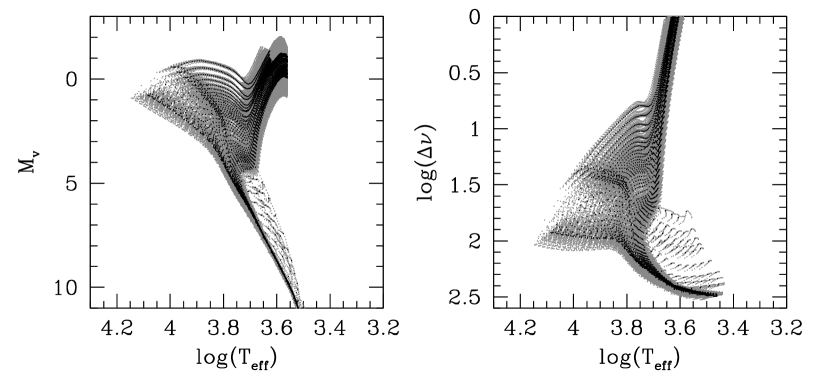
The grid of evolutionary models used are from the Yale-Yonsei (YY) isochrones (see Demarque et al. 2004 and references therein). The models were constructed with a mixing length parameter of $\alpha=1.7431$, OPAL high temperature opacities (Rogers & Iglesias 1995; Iglesias & Rogers 1996) and Alexander & Ferguson (1994) low temperature opacities. The OPAL equation of state (Rogers et al. 1996) was used. The models include diffusion. Core overshoot of $0.2H_{p}$ is included. The models assume the solar mixture of Grevesse & Noels (1993) and the YY solar model has $(Z/X)_{\odot}=0.0243$ and $Y=0.2356$. Higher $Z$ models were made assuming $\Delta Y/\Delta Z=2$. We use the models where the conversion of luminosities to absolute visual magnitude was made using the colour tables of Lejeune et al. (1997).

Figure 3.— (a) Models that contribute to the likelihood function when the central parameter values for BiSON data are used (black points). Points in grey show rest of the models in the grid. (b) The value of the likelihood function for BiSON data plotted as a function of radius. The vertical line marks the centre of gravity of the function. (c) The 10000 models obtained by adding Gaussian errors to the central BiSON values. The centre of gravity of likelihood function of each model forms the distribution function we use to determine the final value of the radius, and errors therein.

The grid of YY models that we have used have [Fe/H] of 0, $\pm 0.05$, $\pm 0.1$, $\pm 0.15$, $\pm 0.20$, $\pm 0.25$, $\pm 0.3$, $\pm 0.4$, and $\pm 0.5$ (where ${\rm[Fe/H]}=\log(Z/X)-\log(Z/X)_{\odot}$). The helium abundance of these models were determined assuming $\Delta Y/\Delta Z=2$. We have also restricted the grid to models with ages between $0.02$ and $14\,\rm Gyr$. The lower age limit ensures that we do not have too many pre-main sequence models, although we do not avoid them completely. We show the grid we use in Figure 2. There are about 95000 models in the grid.

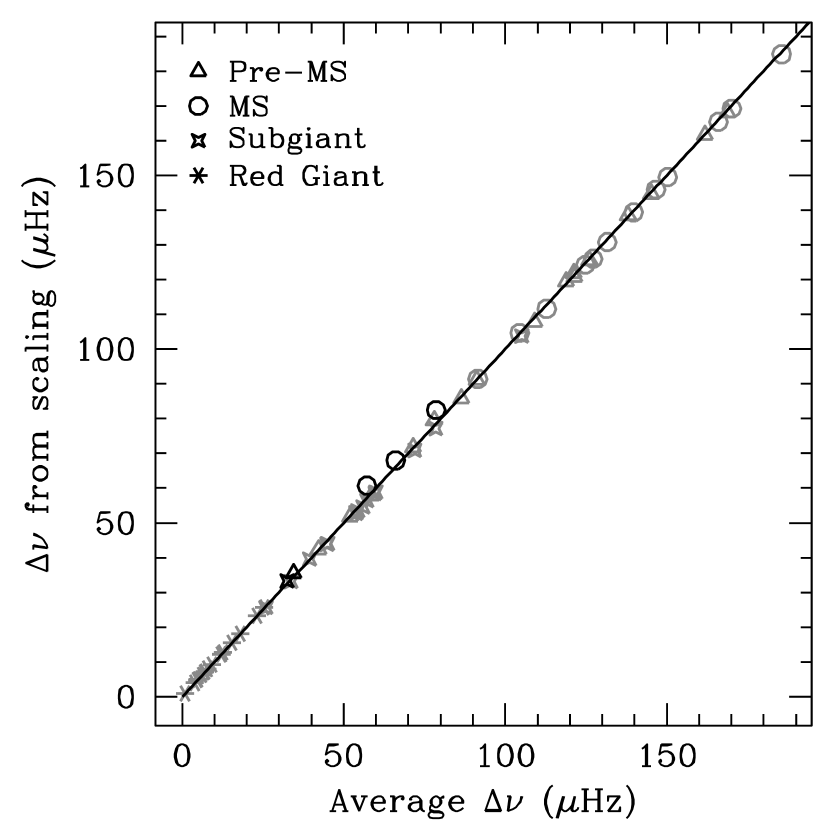
The average large frequency spacings $\Delta\nu$ of these models were estimated by simply scaling from the average solar value, using the aforementioned $(M/R^{3})^{1/2}$ scaling. The alternative would be to first calculate the pulsational frequencies of each model, and from these determine an average large frequency spacing. However, it turns out that the simple scaled values are more than adequate for this work, as can be seen from Figure 2 where we compare for a representative subset of models the large spacing obtained from the scaling relationship to the actual average large spacing from the calculated frequencies. The scaling relation clearly works well. A small deviation is seen for some of the hotter models. This does not concern us much since such hot stars are unlikely to show pulsations.

When we also made use of the frequency of maximum oscillation power, $\nu_{\rm max}$, as part of the input parameter set we estimated its value for each model by again scaling from the average solar value of $3100\,\rm\mu Hz$ using the aforementioned $M\,R^{-2}\,T_{\rm eff}^{-1/2}$ scaling.

The first key step of our method is based on generating 10,000 input parameter sets by adding different random realisations of Gaussian noise to the actual (central) observational input parameter set described at the beginning of this section. This is to allow us to make a proper determination of the errors involved. The use of these randomly perturbed parameter sets also allows us to account for the fact that the relation between the radius of a star and its other properties, such as $T_{\rm eff}$, metallicity and luminosity, is extremely non-linear. Thus, while the 10,000 perturbed parameter sets are created by adding Gaussian noise, the distribution of radii obtained from the perturbed sets does not usually have a Gaussian distribution. The distribution of radii obtained from the central parameter set and the 10,000 perturbed parameter sets is what we refer to in the rest of the paper as the “distribution function.” We settled on the number 10,000 as a compromise between obtaining an eventual smooth distribution of radii in a reasonable computational time, given one set of input variables.

For the central input parameter set and each of the perturbed sets we calculate the likelihood, ${\cal L}$, for models within 3$\sigma$ of the variables of each set. Note that we only choose models that have characteristics within 3$\sigma$ of all the variables. We have a pre-defined minimum over which we calculate the likelihood to avoid problems associated with a discrete grid of models. We find that the $\pm 3\sigma$ limit is sufficient, with the added benefit that it saves on computer time, since fewer models are involved (e.g., results obtained using $\pm 3\sigma$ limits lie well within the errors of those given for the $\pm 4\sigma$ limits). For the cases we have described below, a few hundred of the 95000 models contribute to the likelihood function when seismic constraints are present. In the absence of seismic constraints, the number of models that contribute to the likelihood function rises to a few thousand.

The likelihood can be described as a function of the radius of the model that is used to calculate it. Since we use a discrete grid of models, we obtain a discrete likelihood distribution function, i.e., a distribution function made up of calculated values of ${\cal L}$ for each of the tested models from the discrete model grid. Fitting a functional form and then determining the maximum likelihood is time consuming, and using the maximum of the distribution function of ${\cal L}$ gives biases that vary across the HR diagram. We therefore define the inferred radius of a given set of inputs to be the centre of gravity of the distribution function. Once we have inferred the radius for each of the 10,001 variable sets (again: one central set and 10,000 perturbed sets), we can plot the distribution function of the radii (see below). We choose the second quartile point of the function as the final value of the radius and the inter-quartile distances as the errors on the solution.

To test whether our method works, we first tried to determine the solar radius using the solar large spacing obtained from solar $\ell=0$ frequencies measured by the Birmingham Solar-Oscillations Network (Chaplin et al. 1996). In particular we use the mode set BiSON-1 described in Basu et al. (2009) to determine an the average large spacing calculated between 2.47 mHz and 3.82 mHz for use as a seismic input parameter. The interval was chosen to be roughly ten large spacings centred around the frequency of maximum power. This choice is prompted by what we can expect from Kepler in the Survey Phase. For the purposes of determining likelihood functions ${\cal L}$, and subsequently the distribution function of these ${\cal L}$, we assumed that the Sun has a parallax of $8.9\pm 2.2$ mas, and that the errors in the effective temperature, $\log(Z/X)$ and $\Delta\nu$ are 200 K, 0.2 dex and 0.56 $\mu$Hz, respectively. We also conducted a second exercise were we reduced all the errors by a factor of two. These errors are representative of a “typical” solar-like main-sequence target for Kepler (see also Section 5 below). Computed parallaxes of our tests were fixed according to the known apparent magnitude range for selected solar-like Survey Phase targets, i.e., roughly $V=8$ to $V=11.5$. Note that the precision in the parallax has been chosen to be similar to that in the existing Hipparcos catalogue (at the same apparent magnitude), very likely a pessimistic estimate of the precision we might expect to obtain from Kepler astrometry.

Figure 4.— Results obtained in our attempt to infer the solar radius using the large frequency spacings from BiSON data. We plot the distribution function as a function of the relative error (in %) of the results for two different error distributions. The ‘larger’ error distribution assumes that $\sigma(T_{\rm eff})=200$K, $\sigma(\log(Z/X)=0.2$, $\sigma(\pi)=2.2$mas, $\sigma(\Delta\nu)=0.56\mu$Hz and $\sigma(\nu_{max})=125\mu$Hz. The ‘smaller’ error-distribution assumes that the errors in each of the parameters was exactly half that in the ‘large’ distribution. Note that the distributions are asymmetric, a result of the highly non-linear relationship of stellar radii to their other properties. The inferred solar radius from the two distributions is noted in the figure. As can be seen, the statistical errors are much larger than the systematic error in the results.

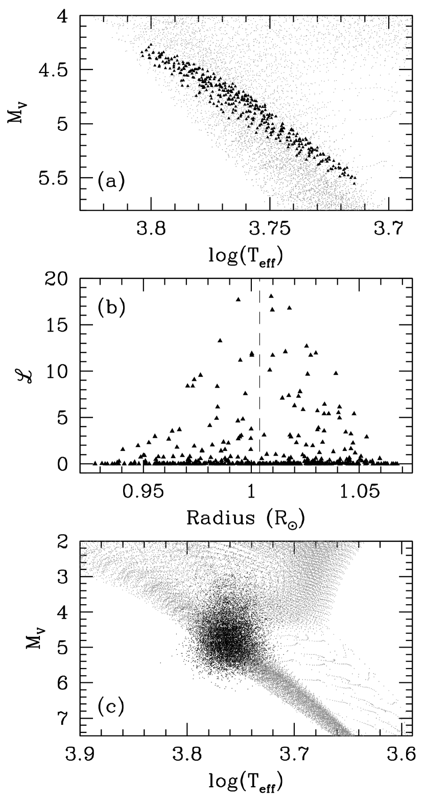
Since our initial aim was to check whether the method works, rather than to assess the effect of errors, we did not add random errors to the input parameters (i.e., the true, underlying input parameters), which would have more closely mimiced the case of real observations. The estimated errors on the input parameters were used only to choose the grid models for the likelihood function, and to generate the randomly perturbed models (see above) used to calculate the distribution function. Section 5 describes the result of an exercise where data with added random errors were used as inputs. Figure 3(a) shows the models of our grid that were used to calculate the likelihood function for the central BiSON values, in the larger error case; Figure 3(b) shows the values of the likelihood function against the radius of the models. 390 models contribute to the likelohood function. As can be seen, the function is well peaked, however, the discrete nature of the grid makes the process of finding the location of the maximum rather unstable (and stable ways are time-consuming and unpractical given, the large volumes of real Kepler data we expect), hence we choose to use the centre of gravity of the distribution, which in the figure is indicated by the vertical line. Figure 3(c) shows the 10,000 models generated to construct the distribution function. The distribution function is constructed by first calculating the likelihood function for each of the models and finding the centre of gravity of each function.

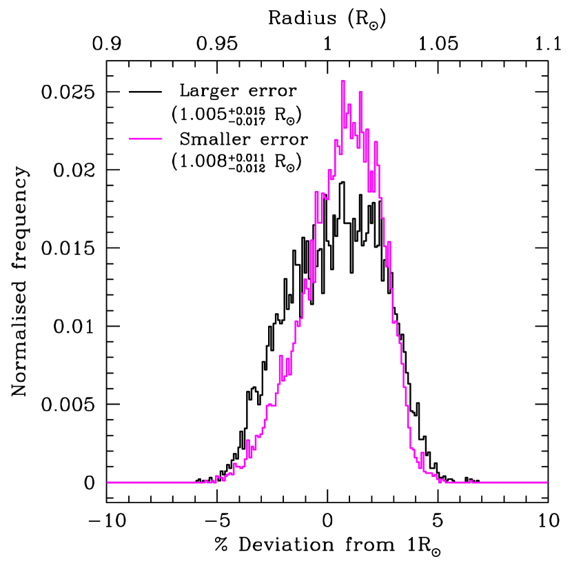
The two distribution functions are plotted in Figure 4. We have plotted the distribution functions against the deviation from $1\,R_{\odot}$ to give a clearer understanding of the errors. The radius can be read from the top of the figure. The first thing to note is that the distribution functions are definitely not Gaussian, and are asymmetric. This is expected given the non-linear relationship between the radius of a star and its temperature, metallicity and luminosity. The solar radius we obtain from this exercise is $1.005^{+0.015}_{-0.017}R_{\odot}$ for the large error case and $1.008^{+0.011}_{-0.012}$ for the smaller error case. As mentioned earlier, the solution is the second quartile point of the distribution and the errors represent the distance to the first and third quartile points. Thus we are able to determine successfully the solar radius, demonstrating that the method works. In the following section we examine the behaviour of the distribution function for stars at various stages of their evolution and the effect of the input errors on the results.

3. Systematic tests of the algorithm

To determine what parameters affect radius determination the most, we performed a series of tests with different models. The models are listed in Table 1. We consider models at six different positions on the HR diagram, starting at the lower main sequence, right up to the red giant branch. The models used in this section are similar to the calibration models used. The effect of having different models is shown in subsequent sections. We use this section to examine the rôle of the various input parameters and the errors on those parameters.

Table 1Characteristics of the models used to test the radius-finding technique

Name	$Z/X$	$T_{\rm eff}$	$M_{\rm V}$	$\Delta\nu$	$\nu_{\rm max}$	Radius	Comments
		(K)		($\mu$Hz)	($\mu$Hz)	(R⊙)
Star 1	0.020	4530	7.38	225.81	6164	0.62	Main sequence star
Star 2	0.051	5175	5.84	172.41	4517	0.83	Main sequence star
Star 3	0.036	5778	4.85	142.15	3456	0.99	Near turn-off
Star 4	0.025	6372	3.17	170.52	1396	1.71	Almost sub giant
Star 5	0.013	6159	2.27	133.73	1541	2.84	Sub giant
Star 6	0.051	4410	2.20	102.20	121	21.44	Red giant

Table 2Assumed errors on stellar parameters

	Error 1	Error 2	Error 3
Assumed parallax (mas)	18.5	8.9	5.4
Parameter		1$\sigma$ error in parameter
$T_{\rm eff}$ (K)	200	200	200
$\log(Z/X)$	0.2	0.2	0.2
$\Delta\nu$ ($\mu$Hz)	0.30	0.56	1.89
$\nu_{\rm max}$ ($\mu$Hz)	80	125	285
$\pi$ (mas)	1.2	2.2	3.6

We use three sets of errors in the input parameters, which are listed in Table 2. The errors in the non-seismic parameters, particularly $T_{\rm eff}$ and $Z/X$, are motivated by what are believed to be typical errors in the Kepler Input Catalogue (KIC). There are cases where the metallicity measurement is suspect, and hence we also determine what happens if we do not use knowledge of the metallicity. We assume that the apparent magnitude of the star is known exactly and that all the error lies in the parallax measurement. However, since most KIC stars do not have accurate parallaxes, we also determine what happens to the radius determination if we do not know the parallax at all. The errors in the seismic variables are roughly what is expected from a month of Kepler data.

Figure 5.— The influence of seismic parameters on the radius determination. Note the large change in the scale of the abscissa (i.e., the change in the uncertainty in the estimated radius) once we start using seismic observables. Panels (a), (b) and (c) show the distribution function plotted as a function of the percentage error in radius for Star 1, Star 3, and Star 5 respectively, when only the non-seismic variables $T_{\rm eff}$, $Z/X$, apparent magnitude $V$ and parallax $\pi$ are used. Error distribution Error 2 was used. Panels (d), (e) and (f) show the results when seismic parameter $\Delta\nu$ is used (magenta lines, grey in the print version), as well as what happens when both $\Delta\nu$ and $\nu_{\rm max}$ (black lines). We plot the distribution function as a function of the percentage deviation from the actual result to make it easier to gauge both systematic error (shift in the peak of the distribution function away from zero) and statistical error (the width of the function).

Figure 6.— The distribution function obtained for the 6 test stars (Table 1) when the errors listed in Table 2 are used. The thick black line is for Error 1, thin black line for Error 2 and magenta line (grey line in the print version) for Error 3. Note that not only do the distribution functions become wider, implying larger statistical errors, when the errors in the inputs are increased the systematic errors increase too.

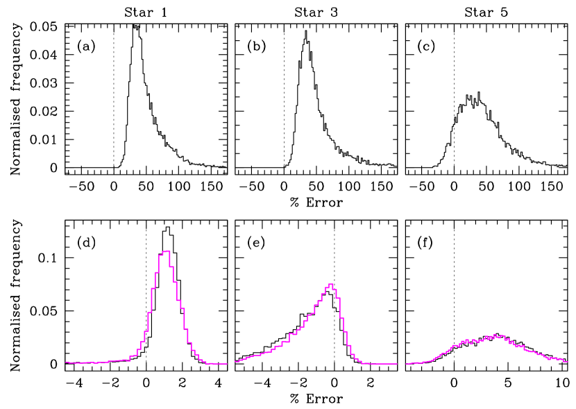
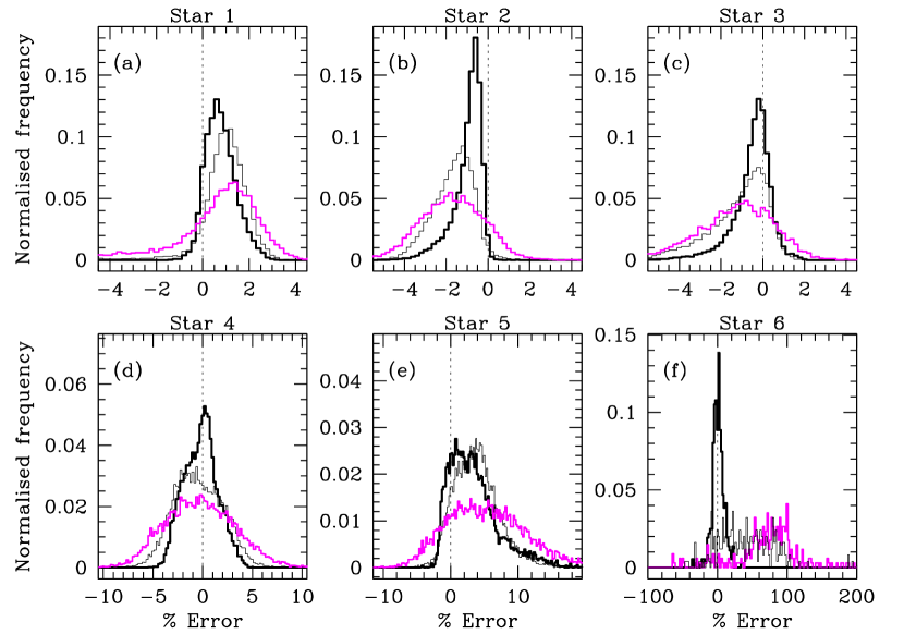
Figure 6 shows the distribution functions obtained for three of the stars when we do not use seismic inputs, and for when we do. The results are for Error 2 (cf. Table 2). As is clear, using only conventional variables ($T_{\rm eff}$, $Z/X$, $V$ and $\pi$) gives radius errors that can be 50 % or higher. When just the large spacing ($\Delta\nu$) is added to the list of inputs, the errors are brought down to less than 5%. Adding the frequency of maximum mode power ($\nu_{\rm max}$) helps a bit more, but the change is not as spectacular.

Figure 6 shows the effect of the three error distributions (Errors 1, 2 and 3) on the resultant distribution function. We remind the reader that the difference between the three errors lies in differences in the assumed parallax, and errors therein, as well as differences in the errors of the seismic variables. As can be seen from the figure, as expected, the distribution with the smallest errors does the best. Increasing errors does not merely widen the distribution function (denoting larger statistical errors in the solution), it also shifts the peak away from the real solution (denoting systematic errors). The situation becomes particularly bad for evolved stars. We fail dismally in the case of the red giant (Star 6) to get any sensible result for Errors 2 and 3. As we show later, estimates of effective temperature and absolute magnitudes need to be good to be able to get radii of red-giants accurately. Given that many red giants in the Kepler sample are expected to be bright enough to obtain individual frequencies even from relatively short time series (mode amplitudes will be significantly higher than in the less luminous main-sequence targets), detailed modelling of the individual frequencies should give better estimates of the radii of these stars.

3.1. The effect of input errors

Our radius-determination method uses a number of inputs, and the errors in the inputs affect the final result. We determine the effect of errors in the inputs by comparing the distribution functions obtained with Error 2 with those obtained by reducing the error in each input variable one by one.

Figure 7.— The effect of error in $\Delta\nu$. We show the distribution function obtained when the error in $\Delta\nu$ is reduced by a factor of two (black line). The original distribution, obtained with Error 2 (Table 2) is shown in magenta (grey).

Figure 8.— The effect of the error in $\nu_{\rm max}$. We show the distribution function obtained when the error in $\nu_{\rm max}$ is reduced by a factor of two (black line). The original distribution, obtained with Error 2 is shown in magenta (grey).

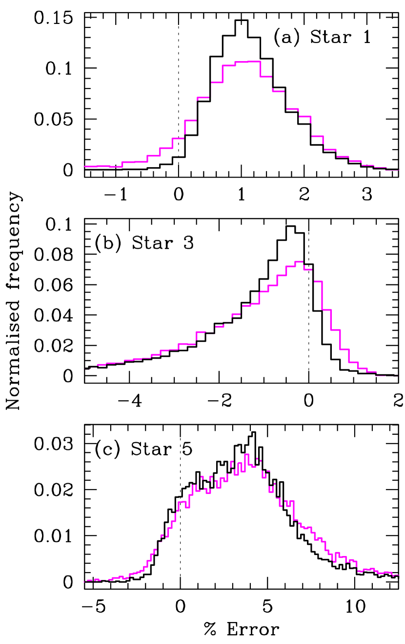
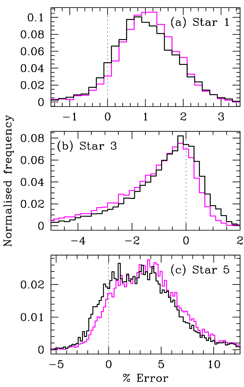
The effect on the distribution function of errors in the seismic variables, $\Delta\nu$ and $\nu_{\rm max}$, is shown in Figures 8 and 8, respectively. The error in $\Delta\nu$ was reduced from $0.56\mu$Hz to $0.28\mu$Hz. As can be seen, reducing the error in $\Delta\nu$ makes the distribution functions narrower, and hence the results more precise. The effect is marked for main-sequence and turn-off stars, but is minimal for sub giants and red giants. As we shall show later, the precision in $T_{\rm eff}$ and $(Z/X)$ is much more important for sub giants, while the precision of the parallax is extremely important for red giants. The effect of the precision of $\nu_{\rm max}$ is minimal, unless the relative precision is of the same order as that of $\Delta\nu$.

Figure 9.— The effect of the error in $T_{\rm eff}$. The distribution functions are plotted as a function of the percentage error, including when $T_{\rm eff}$ is not used at all (thin black line) and when the error in $T_{\rm eff}$ is reduced by a factor of two (black lines) compared to Error 2 (magenta, grey in the print version).

Figure 10.— The effect of the error in $Z/X$. The distribution functions are plotted as a function of the percentage error in radius, including when we disregard $Z/X$ altogether (magenta line, thinn grey in the print version) compared to the original result (thin black line). The distribution shown in the thick black line is obtained when errors in $\log(Z/X)$ are reduced by a factor of two compared to what was used for the dotted distribution. The distribution in green (thick grey in the print version) is what is obtained if we assumed that the star has a solar metallicity, even if it does not.

Figure 11.— The effect of the error in the parallax $\pi$. We show the distribution function obtained when the error in $\pi$ is reduced by a factor of two (black line). The original distribution, obtained with Error 2, is shown in magenta (grey).

Figure 12.— The summary of our results with the six test models. We plot the percentage error in each of the results. The panels are for the three error distributions (Table 2). Each star is indicated by a different colour and the symbols denote the combination of inputs used.

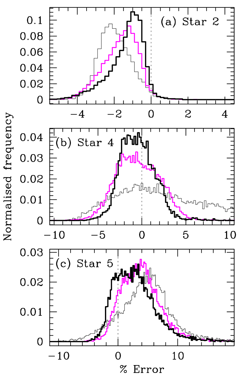
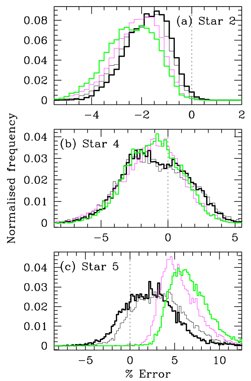
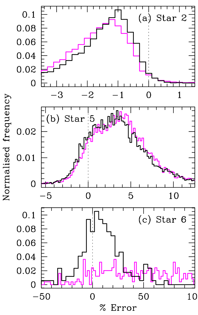
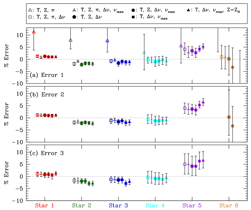
Figure 10 examines the effect of $T_{\rm eff}$ on the results. As can be seen, failure to use $T_{\rm eff}$ is not an option. Decreasing errors in $T_{\rm eff}$ by a factor of two, down to 100 K, increases both the accuracy and precision of the results and additional improvement is obtained by decreasing $\sigma(T_{\rm eff})$ further. The rôle of $T_{\rm eff}$ becomes particularly important in turn-off and post-main-sequence stars where a small change in effective temperature is accompanied by a large change in radius.

The effect of metallicity is shown in Figure 10. We obtained the distributions using Error 2 errors with and without $Z/X$. We also tried reducing the error in $\log(Z/X)$ by a factor of two. The last case we tried assumed that the star has solar metallicity. This was prompted by the fact that the metallicity distribution of solar neighbourhood stars is peaked at very nearly solar metallicity. Our results show, however, that not using $Z/X$ at all gives better results than assuming solar metallicity. The difference is slight for main-sequence stars, but glaring for evolved stars. We find that we cannot get a good radius measurement for evolved stars without a good knowledge of their metallicity.

Figure 12 shows the effect of errors in the parallax. Reducing parallax errors does not affect the results of main-sequence stars and most sub giants too much. It does make a very large difference though in the case of red giants where the luminosity is basically determined by the radius given their narrow $T_{\rm eff}$ range. In the case of main-sequence stars, the effect of even having a parallax is small. This is good news for initial analysis of Kepler data, given that most of the stars in KIC do not have reliable parallaxes (though, as noted previously, we expect eventually to get parallax determinations from the Kepler data).

Figure 12 summarises our results for the six test stars. We show results for each of the three error distributions as well as the results of using (or not using) certain inputs. We plot the deviation of the inferred radius from the actual radius of the model; thus a difference from zero indicates immediately the systematic error in the result, while the error bars indicate the statistical errors. It can be seen that by using seismic inputs we can determine the radius of main sequence stars to within 1 to 2 %. The error in the sub giants is somewhat higher, here about 5 %. We fail pretty badly in the case of the red giant, except when the input errors are small (i.e., the Error 1 case). The figure shows the non-seismic results too: except for the case of Error 1, the error in those results always exceeds 15 %. The figure also shows that knowledge of $T_{\rm eff}$ and the seismic variables is sufficient to allow a good determination of the radii of main sequence stars. More information is required for sub giants and red giants — knowledge of $Z/X$ for sub giants, and both $Z/X$ and luminosity (i.e., apparent magnitude and parallax) for red giants. A good knowledge of the parallax is essential to get red giant radii correctly.

4. Possible sources of systematic errors

There are two possible sources of systematic errors in the radius determination, one is the so called “surface term” and the other is the effect of the mixing length parameter. We examine both these sources in this section.

Figure 13.— The frequency differences between several solar models and solar frequencies obtained from BiSON observations, plotted as a function of the frequency of the mode. Differences for $\ell=0$-$3$ modes are shown. The predominant frequency-dependent trend in the difference is a result of near-surface errors in modelling and is commonly referred to as the “surface term”. Note how the different models have very different surface terms.

4.1. The surface term

Stellar models do not represent the near-surface layers of stars very well. Among the problems is the use of the mixing length approximation to model convection. While this approximation works well in regions of efficient convection, it does not in regions where convection is not efficient, i.e., the near-surface layers. The structure of the superadiabatic layer is incorrect (Nordlund & Dravins 1990; Freytag et al. 1996; Abbett et al. 1997, etc.). In addition, stellar models do not include turbulent pressure that arises from convection, neither do they include the contribution due to turbulent kinetic energy. All these factors lead to errors in the models. Near-surface errors of this kind lead to a frequency-dependent error in the frequencies (see e.g., Christensen-Dalsgaard & Berthomieu 1991) usually referred to as the “surface term”. Differences in near-surface opacities also contribute. To the contribution due to improper modelling is added the fact that frequencies of models are calculated assuming that they are adiabatic, another surface term since that is where adiabaticity breaks down.

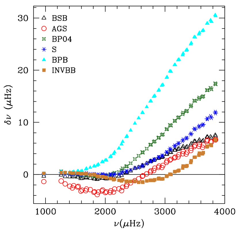
The surface term for various published solar models can be seen in Figure 13. The models are listed in Table 3. This figure shows frequency differences for modes with $\ell=0,1,2$ and $3$ between the models and the solar frequencies in the aforementioned BiSON-1 set, plotted as a function of frequency. As can be seen, the frequency differences are predominantly a function of frequency; furthermore, different models have different surface terms. Methods have been developed by helioseismologists to deal with the surface term in solar data (e.g., Dziembowski et al. 1990). Kjeldsen et al. (2008) have also recently proposed an empirical method for constraining the surface term using asteroseismic data only when estimates of individual mode frequencies are available. However, this is not an option for those Kepler Survey Phase targets where we can only extract an estimate of the average large frequency spacing, and cannot extract robust estimates of individual frequencies (covering several radial orders). Thus we might reasonably expect the radius determination in these stars to be affected, because of the effect of the surface term.

Table 3The effect of the “surface term” — results for various solar models

Model	Comments	Inferred Radius ($R_{\odot}$)
BSB	Model BSB(GS98) of Bahcall et al. (2006)	$1.0023_{-0.0166}^{+0.0135}$
AGS	Model BSB(AGS05) of Bahcall et al. (2006)	$1.0018_{-0.0169}^{+0.0133}$
BP04	Model BP04 of Bahcall et al. (2005)	$0.9997_{-0.0180}^{+0.0135}$
S	Model S of Christensen-Dalsgaard et al. (1996)	$1.0014_{-0.0172}^{+0.0132}$
BPB	Model STD of Basu et al. (2000)	$0.9961_{-0.0188}^{+0.0139}$
INVBB	Seismic model of Antia (1996)	$1.0023_{-0.0166}^{+0.0135}$

To examine how the surface term can affect radius determination using the large frequency spacings, we calculated the average large spacings for each of the solar models shown in Fig. 13 and tried to determine their radii with the same error-distribution as Error 2. Although the large spacings of the models do not include all effects of the surface term, since they too are mixing-length models, they are nonetheless sufficiently different from the calibration models used in the radius search method. The results are listed in Table 3. As can be seen, at least for these models, the differing surface terms do not affect the results much, and the systematic error is much less than 1 %, and smaller than the statistical error. We do not therefore believe that we need to be worried about the surface term when dealing with data from the Kepler survey phase. The results are, however, better than the BiSON results discussed in Section 2 and perhaps we should consider those results as an indication of what systematic errors the surface term introduces.

4.2. The mixing length

The radius of a stellar model depends on the mixing length parameter used to construct the model. Unfortunately, there is no method to determine what the mixing length parameter should be: usually the mixing length parameter needed to reproduce the solar radius at the solar age is used for models of other stars too, and it is quite possible that this is not the correct thing to do. In fact simulations of convection suggest that the mixing length parameter varies across the HR diagram (e.g. Ludwig et al. 1999, 2002; Robinson et al. 2004). All the calibration models here were, of course, constructed with the solar value of the mixing length, and hence it is possible that we will get erroneous results for some stars. To judge how badly we could fail, we test out our method using models constructed with mixing lengths that are different from the one used to construct our calibration models.

Table 4Characteristics of the models with different mixing length parameters

	$Z/X$	$T_{\rm eff}$	$M_{\rm V}$	$\Delta\nu$	$\nu_{\rm max}$	Radius	Comments
		(K)		($\mu$Hz)	($\mu$Hz)	(R⊙)
$\alpha=1.2H_{p}$
Test 1-1	0.024	5360	5.11	123.56	2902	1.06	Main sequence star
Test 1-2	0.024	5386	4.54	185.40	1769	1.36	Near turn-off
Test 1-3	0.024	5219	4.30	163.77	1218	1.65	Sub giant
$\alpha=2.4H_{p}$
Test 2-1	0.024	6059	4.70	146.53	3426	0.95	Main sequence star
Test 2-2	0.024	6128	4.22	109.29	2307	1.15	Near turn-off
Test 2-3	0.024	5613	3.87	162.60	1145	1.67	Sub giant

Figure 14.— Distribution functions for the the six models that have different mixing length parameters than the calibration models. The models are summarised in Table 4. The thick black, thin black and magenta (grey) lines correspond to Errors 1-3 (Table 2) respectively.

Figure 15.— The summary of our results for the six models with different mixing length parameters. The black, red and blue points are the results for the different error distributions, Errors 1-3 respectively. The filled symbols are for the results when all inputs (i.e., $T_{\rm eff}$, $Z/X$, $\pi$, $\Delta\nu$ and $\nu_{\rm max}$) are used, the open symbols are the result of not using $\nu_{\rm max}$.

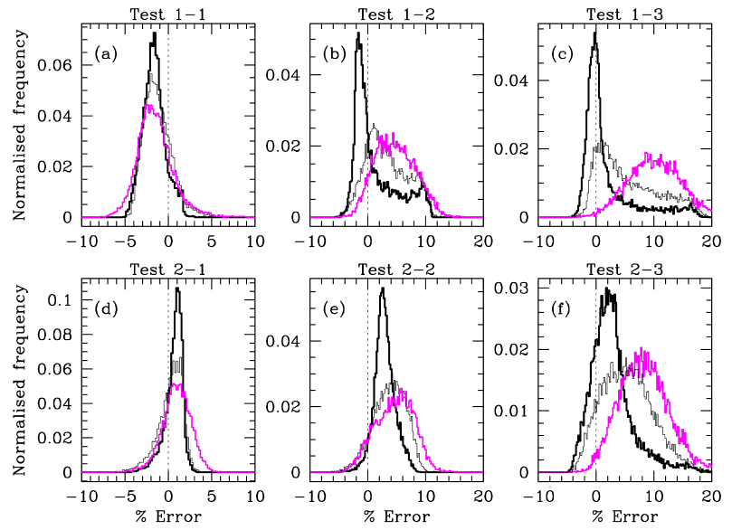
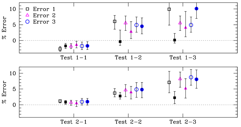
We use a set of six models constructed with two different mixing lengths. The models are listed in Table 4. For each mixing length we have one main sequence, one turn-off and one sub-giant model. Given our failure with red giants in Section 3, we do not try any here. We use the same error distributions as before, i.e., the ones in Table 2. The distribution functions obtained for the six models are shown in Figure 15. We used all inputs ($T_{\rm eff}$, $Z/X$, $V$, $\pi$, $\Delta\nu$ and $\nu_{\rm max}$) to obtain the distribution functions. We can see that there are indeed shifts in the distribution function away from the true value, when a mismatch of the mixing lengths is present. The shifts are particularly bad for the evolved stars when the errors in the input parameters are large. In the case of main-sequence models, the error is no larger than that for the models used in Section 3. The results in terms of the radii obtained are summarised in Figure 15 where we also show what happens if we do not use $\nu_{\rm max}$. As we can see from the figures, the difference between the inferred and the true radius increases as the star evolves. The difference appears to be at the 1 to 2$\sigma$ level. The largest error we get is about 10 %, which is less than what we would get if we did not have seismic parameters, but is nevertheless quite large. We also see that the extra information in $\nu_{\rm max}$ helps in most cases. Thus there is a distinct possibility that our results obtained with Kepler data for evolved stars will be affected. It will help if the errors in the inputs are as small as possible.

5. Blind tests

The stellar models that we tested in Section 3 were very similar to the calibration models that were used to determine the distribution functions. We did use different models in Sections 4.1 and 4.2, however, as for the work described in Section 3, our inputs were exact, without errors. The nominal errors were used only to generate the models that were needed to determine the distribution function.

As a final check on our methods, we therefore performed a proper “all-up” blind test of the technique involving models constructed with different codes (including different mixing length parameters), errors on the inputs, and a surface term included. To this end, the first author of this paper (SB) was given a series of input parameters by the one of the other co-authors (WJC) to determine the radius of the models. The exact parameters and radii were disclosed later. The actual characteristics of the three asteroFLAG models we used (three of the so-called “asteroFLAG cats”) are listed in Table 5; while the inputs provided for the test are listed in Table 6. We now go on to describe how these input data were generated by WJC.

First, we take the non-seismic inputs, i.e., $T_{\rm eff}$, $\log(Z/X)$, and $\pi$. To the actual $T_{\rm eff}$ and $\log(Z/X)$ we added a random Gaussian deviate that had been multiplied by the uncertainty expected on similar data in the KIC. True values of the parallax, $\pi$, were calculated for two Kepler apparent magnitudes, $V=9$ and $V=10$. As noted previously, an Hipparcos-like uncertainty was then assigned to each parallax, and the true value of the parallax perturbed (in the manner described for $T_{\rm eff}$ and $\log(Z/X)$) before the data were passed to SB.

The seismic inputs came from tests conducted on artificial oscillation power spectra of the three cats, which were designed to mimic observations expected in the Survey Phase. These spectra were made with the asteroFLAG simulator. Full details may be found in Chaplin et al. (2008c) [see also Stello et al. 2009]. Here, we note that the stellar models were generated using the Aarhus stellar evolution code, ASTEC (Christensen-Dalsgaard 2008a), while the oscillation frequencies were calculated using the adiabatic pulsation code ADIPLS (Christensen- Dalsgaard 2008b). The oscillation spectra of the cats differed from those used in Stello et al. (2009) in two important respects. First, the underlying oscillation amplitudes and damping rates were modified to more accurately reflect expected levels for the Kepler observations (e.g., based on experience accumulated from analysing the CoRoT data). Second, artificial spectra were made to simulate those expected from observations lasting one month (i.e., the Survey Phase length), not the 3.5 yr used in Stello et al.

Table 5Characteristics of asteroFLAG blind-test models

Name	Mass	Radius	Age	$\alpha$	$T_{\rm eff}$	$\log(Z/X)$
	($M_{\odot}$)	($R_{\odot}$)	(Gyr)		(K)
Katrina	0.70	0.63	1.000	3.05	4350.03	$-1.67$
Boris	1.00	1.00	4.600	1.99	5777.00	$-1.61$
Pancho	1.40	1.75	1.995	2.03	6351.57	$-1.39$

Table 6Inputs for the blind test on three of the asteroFLAG cats

Name	$T_{\rm eff}$	$\log(Z/X)$	$V$	$\pi$	$\Delta\nu$	$\nu_{\rm max}$
	(K)		(mag)	(mas)	($\mu$Hz)	($\mu$Hz)
Katrina	$4618\pm 200$	$-1.42\pm 0.2$	9	$46.8\pm 1.2$	$227.33\pm 1.89$	$7209.1\pm 285$
Boris	$5676\pm 200$	$-1.31\pm 0.2$	9	$12.5\pm 1.2$	$136.10\pm 0.30$	$3165.4\pm 110$
			10	$8.8\pm 1.7$	$136.29\pm 0.60$	$3138.3\pm 200$
Pancho	$6251\pm 200$	$-1.09\pm 0.2$	9	$8.9\pm 1.2$	$69.51\pm 0.34$	$1684.8\pm 80$
			10	$3.8\pm 1.7$	$69.67\pm 0.56$	$1671.2\pm 125$

Many independent realisations of the oscillation power spectra were made at each $V$, and the spectra analysed with the “Octave” (Birmingham-Sheffield Hallam) Kepler data-analysis pipeline to extract the seismic inputs. This pipeline has been developed as part of the asteroFLAG programme, and will be described in detail elsewhere (Hekker et al., in preparation). We show only inputs for Katrina at $V=9$ because it was hard to extract a robust estimate of the seismic inputs from her artificial oscillation power spectra at $V=10$ (it has the weakest modes of the three cats).

The results of our tests are listed in Table 7, and shown graphically in Figure 16. As can be seen from the figure, we have succeeded in inferring the radii of the cats to within a few percent. We are therefore confident that the Yale-Birmingham method can be used to obtain reliable stellar radii using seismic data from Kepler. The best results are seen for the low-mass main-sequence star, as expected from what we have seen in Section 3.

Table 7Results of the blind test on three of the asteroFLAG cats

Name	Radius	V	Inferred Radius
	(Exact)		(1)	(2)	(3)	(4)	(5)	(6)
	($R_{\odot}$)		($R_{\odot}$)
Katrina	0.63	9	$0.667_{-0.024}^{+0.042}$	$0.630_{-0.004}^{+0.004}$	$0.629_{-0.004}^{+0.004}$	$0.626_{-0.004}^{+0.004}$	$0.627_{-0.004}^{+0.004}$	$0.625_{-0.004}^{+0.004}$
Boris	1.00	9	$1.292_{-0.092}^{+0.112}$	$1.023_{-0.008}^{+0.005}$	$1.027_{-0.006}^{+0.003}$	$1.001_{-0.018}^{+0.013}$	$1.008_{-0.016}^{+0.011}$	$0.985_{-0.016}^{+0.014}$
		10	$1.306_{-0.110}^{+0.170}$	$1.012_{-0.014}^{+0.009}$	$1.014_{-0.013}^{+0.008}$	$1.002_{-0.016}^{+0.012}$	$1.005_{-0.015}^{+0.011}$	$0.983_{-0.013}^{+0.013}$
Pancho	1.75	9	$1.493_{-0.092}^{+0.142}$	$1.746_{-0.017}^{+0.023}$	$1.708_{-0.021}^{+0.027}$	$1.759_{-0.017}^{+0.020}$	$1.732_{-0.028}^{+0.030}$	$1.752_{-0.022}^{+0.018}$
		10	$4.610_{-0.351}^{+0.606}$	$1.752_{-0.021}^{+0.022}$	$1.748_{-0.030}^{+0.025}$	$1.746_{-0.023}^{+0.020}$	$1.737_{-0.030}^{+0.026}$	$1.708_{-0.020}^{+0.026}$

(1) Using $T_{\rm eff},\;Z,\;\pi$; (2) Using $T_{\rm eff},\;Z,\;\pi,\;\Delta\nu,\;\nu_{\rm max}$; (3) Using $T_{\rm eff},\;Z,\;\pi,\;\Delta\nu$

(4) Using $T_{\rm eff},\;Z,\;\Delta\nu,\;\nu_{\rm max}$; (5) Using $T_{\rm eff},\;Z,\;\Delta\nu$; (6) Using $T_{\rm eff},\;Z=Z_{\odot},\;\Delta\nu,\;\nu_{\rm max}$

Figure 16.— The results of the blind tests plotted as the deviation from the true value. Note that in all cases we are able to reproduce the results to within a few percent. The different symbols denote the different combinations of inputs used to obtain the results. The symbols are explained at the top of the figure. The non-seismic inference (Case (1) in Table 7) has not been plotted.

Although we used the same cats as those in used Stello et al. (2009), we cannot directly compare our results with those since the errors we assumed were different (higher in most cases). However, despite that, our results compare favourably, as can be seen if we compare our Table 7 with Table 2 of Stello et al. (2009). In order to facilitate a direct comparison, we put their Katrina input K1, Boris input B1 and and Pancho input P1 through our pipeline and obtained radii of $0.625^{+0.003}_{-0.004}R_{\odot}$ for Katrina, $1.020^{+0.007}_{-0.010}R_{\odot}$ for Boris and $1.717^{+0.030}_{-0.036}R_{\odot}$ for Pancho. The results in Stello et al. (2009) range from $0.602$-$0.682R_{\odot}$ for Katrina, $0.977$-$1.02R_{\odot}$ for Boris and $1.676$-$1.746R_{\odot}$ for Pancho. Thus we compare very well with the other methods. It should be noted that the exercise in Stello et al. (2009) did not include $\nu_{\rm max}$ and hence we did not use it either to determine the radius from inputs K1, B1 and P1.

6. Conclusions

We have described a method to determine stellar radius using a mixture of conventional and seismic variables. We use $\Delta\nu$, the average large frequency spacing, and $\nu_{\rm max}$, the frequency of maximum mode power, as the seismic inputs; while effective temperature, metallicity, the apparent visual magnitude and parallaxes are the “conventional” inputs. We have also performed an error analysis to determine which parameters play the most important rôle in determining the radius using our method.

Our main conclusions are as follows:

• We find that the mere presence of seismic data reduces errors in the inferred radii to a few percent, with main-sequence stars faring better than more evolved solar-type stars.

• We find that for main-sequence stars, a knowledge of the parallax is not important. As long as the effective temperature and the seismic variables are well constrained observationally, we can get results to an accuracy of better than a few percent. Metallicity does not make much difference either for main sequence stars. This is good news as far as Kepler targets are concerned since the parallaxes and metallicities in the Kepler Input Catalogue are known to be suspect, when considered on a star-by-star basis. Insensitivity to the metallicity does not hold for all radius-determination methods, as can be seen in Stello et al. (2009).

• The situation is different for sub giants, and we find that for them we need a good estimate of the metallicity (along with the effective temperature and the seismic parameters) to get a reasonably accurate result. However, we should emphasise that because of the assumed availability of seismic data, we can still infer the radius of these stars to much higher precision than would be possible without those seismic data, no matter how poorly we know the metallicity of the star.

• Robust estimation of the radii of red giants is extremely difficult. The narrow temperature range they occupy, and the sensitive dependence of the radii on luminosity, means that we must have a very precise knowledge of their temperature, and particularly their luminosity (i.e., we need to know their parallaxes very well) to determine their radii accurately. Fortunately, many of the red giants on the Kepler target list will be bright enough to allow extraction of individual oscillation frequencies for these stars, and not just an average large spacing. As a result, it is unlikely that we will have to use our method to determine red giant radii.

• Our tests show that the much-feared “surface term” should not hamper the effort to determine stellar radii accurately from the Kepler survey phase data. Tests with both error-less data and simulations of what we can expect from Kepler show that the surface term has a minimal effect on the inferred radius (at the level of precision expected for the survey phase). While uncertainties in the mixing length can cause errors, the effect is small, particularly for main sequence stars.

• Finally, blind tests on three of the “asteroFLAG cats”, using data simulated to match the kinds of data expected from the survey phase of Kepler, verify that it will be possible to infer stellar radii successfully with our method to a typical precision of just a few percent.

References

- Abbett et al. (1997) Abbett, W. P., Beaver, M., Davids, B., Georgobiani, D.; Rathbun, P., Stein, R. F., 1997, ApJ, 480, 395
- Alexander & Ferguson (1994) Alexander, D. R., & Ferguson, J. W. 1994, ApJ, 437, 879
- Antia (1996) Antia, H.M., 1996, A&A, 307, 609
- Appourchaux et al. (2008) Appourchaux, T., Michel, E., Auvergne, M., et al. 2008, A&A, 488, 705
- Baglin et al. (2006) Baglin, A., Michel, E., Auvergne, M., and the CoRoT Team, 2006, in: Beyond the Spherical Sun, SOHO18/GONG 2006/HELAS I, eds. K. Fletcher, M. J. Thompson, ESA SP-624, Sheffield, UK, p. 34
- Bahcall et al. (2005) Bahcall, J.N., Basu, S., Pinsonneault, M., Serenelli, A. 2005, ApJ, 618 1049
- Bahcall et al. (2006) Bahcall, J.N., Serenelli, A., Basu, S. 2006, ApJS, 165, 400
- Basu et al. (2000) Basu, S., Pinsonneault, M.H., Bahcall, J.N. 2000, ApJ, 529, 1084
- Bedding & Kjeldsen (2003) Bedding T. R., Kjeldsen H., 2003, PASA, 20, 203
- Bedding et al. (2007) Bedding T. R., Kjeldsen, H., Arentoft, T., 2007, ApJ, 663, 1315
- Borucki et al. (2008) Borucki, W., Koch, D., Basri, G., Batalha, N., Brown, T., Caldwell, D., Christensen-Dalsgaard, J., Cochran, W., Dunham, E., Gautier, T. N., Geary, J., Gilliland, R., Jenkins, J., Kondo, Y., Latham, D., Lissauer, J. J., Monet, D. 2008, in IAU Symposium, Vol. 249, IAU Symposium, 17
- Brown et al. (2005) Brown, T. M., Everett, M., Latham, D. W., Monet, D. G., 2005, in Bulletin of the American Astronomical Society, Vol. 37, Bulletin of the American Astronomical Society, 1340
- Chaplin et al. (1996) Chaplin W. J., Elsworth Y., Howe R., Isaak G. R., McLeod C. P., Miller B. A., New R., van der Raay H. B. & Wheeler S. J., 1996, SolPhys, 168, 1
- Chaplin et al. (2008a) Chaplin W. J., Appourchaux T., Arentoft T., et al., 2008a, JPhCS, 118, 012048
- Chaplin et al. (2008b) Chaplin, W. J., Houdek, G., Appourchaux, T., Elsworth, Y., New, R., & Toutain, T. 2008b, A&A, 485, 813
- Chaplin et al. (2008c) Chaplin W. J., Appourchaux T., Arentoft T., et al., 2008c, AN, 329, 549
- Christensen-Dalsgaard & Berthomieu (1991) Christensen-Dalsgaard, J., Berthomieu, G., 1991, in Theory of solar oscillations eds Cox, A. N., Livingston, W. C. & Matthews, M., Space Science Series, University of Arizona Press, p. 401
- Christensen-Dalsgaard (1993) Christensen-Dalsgaard J., 1993, in: T. M. Brown (ed.), Proc GONG 1992: Seismic Investigation of the Sun and Stars, ASP. Conf. Ser. vol. 42 (San Francisco ASP), 347
- Christensen-Dalsgaard et al. (1996) Christensen-Dalsgaard, J., et al. 1996, Science, 272, 1286
- Christensen-Dalsgaard et al. (2008a) Christensen-Dalsgaard J., Arentoft T., Brown T. M., Gilliland R. L., Kjeldsen H., Borucki W. J., Koch D., 2008a, CoAst, 157, 266
- Christensen-Dalsgaard et al. (2008b) Christensen-Dalsgaard J., Arentoft T., Brown T. M., Gilliland R. L., Kjeldsen H., Borucki W. J., Koch D., 2008b, JPhCS, 118, 012039
- Christensen-Dalsgaard (2008a) Christensen-Dalsgaard J., 2008a, Ap&SS, 316, 113
- Christensen-Dalsgaard (2008b) Christensen-Dalsgaard J., 2008b, Ap&SS, 316, 13
- Demarque et al. (2004) Demarque, P, Woo,J-H, Kim, Y-C, Yi, S.K., 2004, ApJS, 155, 667
- Dziembowski et al. (1990) Dziembowski, W. A., Pamyatnykh, A. A., & Sienkiewicz, R. 1990, MNRAS, 244, 542
- Freytag et al. (1996) Freytag, B., Ludwig, H.-G., Steffen, M., 1996, A&A, 313, 497
- Grevesse & Noels (1993) Grevesse, S., Noels, A 1993, in Origin and Evolution of the elements, eds. N. Prantzos, E. Vangioni, M. Cassé (Cambridge Univ. Press: Cambridge) p15
- Iglesias & Rogers (1996) Iglesias, C.A., Rogers, F.J. 1996, ApJ, 464, 943
- Kjeldsen & Bedding (1995) Kjeldsen H., Bedding T. R., 1995, A&A, 293, 87
- Kjeldsen et al. (2009) Kjeldsen, H., Bedding, T. R., Christensen-Dalsgaard, J. 2009, in IAU Symposium, Vol. 253, IAU Symposium, p 309
- Kjeldsen et al. (2008) Kjeldsen H., Bedding T. R., Christensen-Dalsgaard J., 2008, ApJ, 683, L175
- Lejeune et al. (1997) Lejeune, Th., Cuisinier, F., Buser, R. 1997, A&A, 125, 229
- Ludwig et al (1999) Ludwig, H.-G., Freytag, B., Steffen, M., 1999, A&A, 346, 111
- Ludwig et al (2000) Ludwig, H.-G., Allard, F., Hauschildt, P.H., 2002, A&A, 395, 99
- Michel et al. (2008) Michel, E., Baglin, A., Auvergne, M., 2008, Sci, 322, 558
- Nordlund & Dravins (1990) Nordlund, Å., Dravins, D. 1990, A&A, 228, 155
- Robinson et al. (2004) Robinson, F.J., Demarque, P., Li, L. H., Sofia, S., Kim, Y.-C., Chan, K. L., Guenther, D. B., 2004, MNRAS, 347, 1208
- Rogers et al. (1996) Rogers, F. J., Swenson, F. J., Iglesias, C. A. 1996, ApJ, 456, 902
- Stello et al. (2009) Stello, D. et al. 2009, A&A, in press (arXiv:0906:0766)