Shear banding and interfacial instability in planar Poiseuille flow

Abstract

Motivated by the need for a theoretical study in a planar geometry that can easily be implemented experimentally, we study the pressure driven Poiseuille flow of a shear banding fluid. After discussing the “basic states” predicted by a one dimensional calculation that assumes a flat interface between the bands, we proceed to demonstrate such an interface to be unstable with respect to the growth of undulations along it. We give results for the growth rate and wavevector of the most unstable mode that grows initially, as well as for the ultimate flow patterns to which the instability leads. We discuss the relevance of our predictions to the present state of the experimental literature concerning interfacial instabilities of shear banded flows, in both conventional rheometers and microfluidic channels.

I Introduction

Complex fluids have internal mesoscopic structure that is readily reorganised by an imposed shear flow. This reorganisation in turn feeds back on the flow field, resulting in strongly nonlinear constitutive properties. In some systems this nonlinearity is so pronounced that the underlying constitutive curve relating shear stress $T_{xy}$ to shear rate $\dot{\gamma}$ in homogeneous flow is predicted to have a region of negative slope $dT_{xy}/d\dot{\gamma}<0$ spenley93 ; spenley96 . In this regime, an initially homogeneous flow is unstable to the formation of coexisting shear bands of differing local viscosities and internal structuring, with band normals in the flow-gradient direction $y$ Yerushalmi70 . The signature of this transition in bulk rheometry is the presence of characteristic kinks, plateaus and non-monotonicities in the composite flow curve rehage91 . Explicit observation of the bands is made using local rheological techniques such as flow birefringence Decr+95 and NMR britton-prl-78-4930-1997 ; callaghan2008 , ultrasound BecManCol04 ; manneville2008 , heterodyne dynamic light scattering SalColManMol03 ; manneville2008 or particle image hu-jr-49-1001-2005 velocimetry. Using these methods, the existence of shear banding has been firmly established in a wide range of complex fluids, including wormlike BRP94 ; callaghan96 ; grand97 ; britton-prl-78-4930-1997 ; berret94a ; schmitt94 ; Capp+97 ; rehage91 ; Decr+95 ; Makh+95 ; BPD97 and lamellar diat93 ; wilkinsOlms2006 ; Bonn+98 ; SalManCol03 ; SalManCol03b ; ManSalCol04 surfactants; side-chain liquid crystalline polymers pujolle01 ; viral suspensions lettinga-jpm-16-S3929-2004 ; dhont-jcp-118-1466-2003 ; telechelic polymers berret-prl-8704–2001 ; soft glasses CRBMGHJL02 ; holmes-jr-48-1085-2004 ; rogers2008 ; polymer solutions HilVla02 ; and colloidal suspensions ChenZAHSBG92 .

Beyond the basic observation of shear banding, experiments with enhanced spatial and temporal resolution have more recently revealed the presence of complex spatio-temporal patterns and dynamics in many shear banded flows BecManCol04 ; holmes-el-64-274-2003 ; lopez-gonzalez-prl-93–2004 ; bandyopadhyay-prl-84-2022-2000 ; ganapathy-prl-96–2006 ; HBP98 ; bandyopadhyay-el-56-447-2001 ; wheeler-jnfm-75-193-1998 ; herle-l-21-9051-2005 ; fischer-ra-39-234-2000 ; azzouzi-epje-17-507-2005 ; decruppe-pre-73–2006 ; SalManCol03b ; Salmon02 ; ManSalCol04 ; HilVla02 ; lerouge-prl-96–2006 ; lerouge2008 ; fardin2009 . In many such cases, the bulk stress response of the system to a steady imposed shear rate (or vice versa) is intrinsically unsteady, showing either temporal oscillations or erratic fluctuations about the average (flow curve) value. Local rheological measurements reveal such signals commonly to be associated with a complicated behaviour of the interface between the bands BecManCol04 ; holmes-el-64-274-2003 ; lopez-gonzalez-prl-93–2004 ; HBP98 ; wheeler-jnfm-75-193-1998 ; herle-l-21-9051-2005 ; fischer-ra-39-234-2000 ; SalManCol03b ; HilVla02 ; lerouge-prl-96–2006 ; lerouge2008 ; fardin2009 . The majority of these measurements have been in one spatial dimension (1D), normal to the interface between the bands. However 2D observations in Refs. lerouge-prl-96–2006 ; lerouge2008 explicitly revealed the presence of undulations along the interface, in a boundary driven curved Couette flow, accompanied by Taylor-like vortices fardin2009 . The undulations were shown to be either static or dynamic, according to the imposed flow parameters.

Theoretically, instability of an initially flat interface between shear bands was predicted in boundary driven planar Couette flow in Refs. fielding-prl-95–2005 ; wilson-jnfm-138-181-2006 ; fielding2007b . In this work, separate 2D studies in the flow/flow-gradient ($x$-$y$) fielding-prl-95–2005 ; wilson-jnfm-138-181-2006 and flow-gradient/vorticity ($y$-$z$) fielding2007b planes revealed instability with respect to undulations along the interface with wavevector in the flow and vorticity directions respectively. In both cases the mechanism for instability was suggested to be a jump in normal stress across the interface hinch-jnfm-43-311-1992 .

While these predictions provide a good starting point, there remains the possibility that the interfacial undulations observed in Refs. lerouge-prl-96–2006 ; lerouge2008 ; fardin2009 originate instead in curvature driven effects such as a bulk viscoelastic instability of the Taylor Couette larson-jfm-218-573-1990 type in the high shear band, as discussed in Ref. fardin2009 . These were neglected in the planar calculations of Refs. fielding-prl-95–2005 ; wilson-jnfm-138-181-2006 ; fielding2007b (Other possibilities, also neglected, include free surface instabilities at the open rheometer edges; and an erratic stick-slip motion at the solid walls of the flow cell. We shall not consider these further in what follows here either.)

In principle, therefore, either (or both) of (at least) two possible mechanisms could underlie the observed interfacial undulations: (i) a bulk viscoelastic Taylor Couette like instability of the strongly sheared band, or (ii) instability of the interface between the bands, driven by the normal stress jump across it. Of these, scenario (i) can only arise in a curved geometry. Experiments in planar shear could therefore in principle help discriminate between these scenarios, by eliminating the curvature required for (ii). However they are technically difficult to implement in a boundary driven setup.

There thus exists a clear need for theoretical predictions in a planar flow geometry that could easily be implemented experimentally. An obvious candidate comprises pressure driven flow in a rectilinear microchannel of rectangular cross section with a high aspect ratio $L_{z}/L_{y}\gg 1$. Indeed, such experiments have recently been performed nghe2008 ; masselon2008 ; submitted , as discussed in more detail below. With this motivation in mind, in this paper we study the planar Poiseuille flow of a shear banding fluid driven along the main flow direction $x$ by a constant pressure drop $\partial_{x}P=-G$. For simplicity we assume the fluid to be sandwiched between stationary infinite parallel plates at $y=\{0,L_{y}\}$, neglecting the lateral walls in the $z$ direction, and so taking the limit $L_{z}/L_{y}\to\infty$ at the outset. Our main contribution will be to show an interface between shear bands to be unstable in this pressure driven geometry, as it is in the boundary driven planar Couette flow studied previously fielding-prl-95–2005 ; wilson-jnfm-138-181-2006 ; fielding2007b . We will furthermore give results for the growth rate and wavevector associated with the early stage kinetics of this instability, as well as the ultimate flow patterns to which it leads.

Figure 1: Left) Dotted line: homogeneous constitutive curve for $a=0.3$, $\eta=0.05$. Thick solid line: composite flow curve for one-dimensional planar shear banded Couette flow (data already published in Ref. fielding-prl-95–2005 ). Selected stress $T_{\rm sel}=0.506$. Thin solid line: parametric plot of local shear stress $T_{xy}(y)=\Sigma_{xy}(y)+\eta\dot{\gamma}(y)=G(\tfrac{1}{2}-y)$ against local shear rate $\dot{\gamma}(y)$ for one-dimensional planar shear banded Poiseuille flow with $l=0.00125$, $G=2.0$.
Right) Halved pressure gradient versus total throughput for one-dimensional planar Poiseuille flow with $a=0.3$, $\eta=0.05$, $l=0.0025$. This shows a kink at the onset of banding at $G/2=T_{\rm sel}$ as expected.

The paper is structured as follows. After introducing the rheological model and boundary conditions in Sec. II, we calculate in Sec. III the one-dimensional (1D) shear banded states that are predicted when spatial variations are permitted only in the flow gradient direction $y$, artificially assuming translational invariance in $x$ and $z$, and accordingly assuming a flat interface between the bands. These form the “basic states” and initial conditions to be used in the stability calculations of the rest of the paper.

In Sec. IV we study the linear stability of these 1D basic states with respect to small amplitude perturbations with wavevector $q_{x}\hat{\mathbf{{x}}}$ in the flow direction. As in the case of boundary driven flow studied previously, we find an undulatory instability of the interface between the bands fielding-prl-95–2005 ; wilson-jnfm-138-181-2006 ; fielding2007b . Results are then presented for the ultimate nonlinear dynamical attractor in this $x$-$y$ plane, from simulations that adopt periodic boundaries in $x$. This exhibits interfacial undulations of finite amplitude that convect along the flow direction at a constant speed. In Sec. V we turn instead to the flow-gradient/vorticity plane $y$-$z$, likewise demonstrating linear instability of the interface with respect to small amplitude perturbations with wavevector $q_{z}\hat{\mathbf{{z}}}$. We also give results for the ultimate nonlinear flow state, which in this plane is steady. Directions for future work, which will include full 3D calculations, are discussed in Sec. VI.

II Model and geometry

The generalised Navier–Stokes equation for a viscoelastic material in a Newtonian solvent of viscosity $\eta$ and density $\rho$ is

$$\rho(\partial_{t}+\mathbf{{v}}.{\bf\nabla})\mathbf{{v}}={\bf\nabla}.(\mathbf{{T}}-P\mathbf{{I}})={\bf\nabla}.(\mathbf{{\Sigma}}+2\eta\mathbf{{D}}-P\mathbf{{I}}),$$ (1)

where $\mathbf{{v}}(\mathbf{{r}},t)$ is the velocity field and $\mathbf{{D}}$ is the symmetric part of the velocity gradient tensor, $({\bf\nabla}\mathbf{{v}})_{\alpha\beta}\equiv\partial_{\alpha}v_{\beta}$. Throughout we will assume zero Reynolds’ number $\rho=0$. The pressure field $P(\mathbf{{r}},t)$ is determined by enforcing incompressibility,

$$\mathbf{{\nabla}}\cdot\mathbf{{v}}=0.$$ (2)

The quantity $\mathbf{{\Sigma}}(\mathbf{{r}},t)$ in Eqn. 1 is the extra stress contributed to the total stress $\mathbf{{T}}(\mathbf{{r}},t)$ by the viscoelastic component. We assume this to obey the diffusive Johnson-Segalman (DJS) model johnson-jnfm-2-255-1977 ; olmsted-jr-44-257-2000

$$(\partial_{t}+\mathbf{{v}}\cdot{\bf\nabla})\,\mathbf{{\Sigma}}=a(\mathbf{{D}}\cdot\mathbf{{\Sigma}}+\mathbf{{\Sigma}}\cdot\mathbf{{D}})+(\mathbf{{\Sigma}}\cdot\mathbf{{\Omega}}+\mathbf{{\Omega}}\cdot\mathbf{{\Sigma}})+2G_{0}\mathbf{{D}}-\frac{\mathbf{{\Sigma}}}{\tau}+\frac{\ell^{2}}{\tau}{\bf\nabla}^{2}\mathbf{{\Sigma}}.$$ (3)

Here $a$ is a slip parameter, $G_{0}$ is a plateau modulus, $\tau$ is the viscoelastic relaxation time, and $\mathbf{{\Omega}}$ is the antisymmetric part of the velocity gradient tensor. The diffusive term ${\bf\nabla}^{2}\mathbf{{\Sigma}}$ is needed to correctly capture the structure of the interface between the shear bands, with a slightly diffusive interfacial thickness $O(l)$, and to ensure unique selection of the shear stress at which banding occurs lu-prl-84-642-2000 .

Within this model we study flow between infinite flat parallel plates at $y=\{0,L_{y}\}$. The fluid is driven in the positive $x$ direction by a constant pressure gradient $\partial_{x}p=-G$, the plates being held stationary. At the plates we assume conditions of zero flux normal to the wall $\hat{\vec{n}}.{\bf\nabla}\Sigma_{\alpha\beta}=0\;\forall\;\alpha,\beta$ for the viscoelastic stress (although other choices are possible adams2008 ), with no slip and no permeation for the fluid velocity. Throughout we use units in which $G_{0}=1,\tau=1$ and $L_{y}=1$. Unless otherwise stated we use a (dimensionless) value $\eta=0.05$, suggested by the experiments of Refs. nghe2008 . We take $a=0.3$, although our results are quite robust with respect to variations in this quantity. An order of magnitude estimate suggests $l=O(10^{-3})$ fielding-epje-11-65-2003 .

III One-dimensional basic state

In this section we discuss the flow curves and shear banded states predicted by 1D calculations that allow spatial variations only in the flow-gradient direction $y$, assuming (often artificially) translational invariance in the flow direction $x$ and vorticity direction $z$. As a warm-up discussion to the case of planar Poiseuille flow (PPF) that forms the primary interest of this paper, we review first the more familiar case of planar Couette flow (PCF).

In steady 1D PCF, the shear stress $T_{xy}$ is uniform across the flow cell. This follows trivially from solving Eqn. 1 in this geometry. Within the (often artificial) assumption of a similarly homogeneous shear rate field, corresponding to a velocity field $\mathbf{{v}}=\dot{\gamma}y\hat{\vec{x}}$, the constitutive relation is then given by $T_{xy}(\dot{\gamma})=\Sigma_{xy}(\dot{\gamma})+\eta\dot{\gamma}$, where $\Sigma_{xy}(\dot{\gamma})$ follows as the $xy$ component of the solution of Eqn. 3 obtained by assuming stationarity in time and homogeneity in space. See the dotted line in Fig. 1 (left). For an applied shear rate in the region of negative slope $dT_{xy}/d\dot{\gamma}<0$, homogeneous flow is predicted to be linearly unstable with respect to the formation of shear bands. The steady state composite flow curve is then shown by the thick solid line in the same figure. For shear stresses $T_{xy}<T_{\rm sel}$ (resp. $T_{xy}>T_{\rm sel}$), where the selected stress $T_{\rm sel}=0.506$ for the particular choice of parameters in Fig. 1, the system shows homogeneous flow on the low shear (resp. high shear) branch of the constitutive curve. Applying a value of the shear rate $\overline{\dot{\gamma}}$ in the window between these branches, we obtain shear bands that coexist at the selected stress $T_{xy}=T_{\rm sel}$.

Figure 2: Left) Velocity profiles in one-dimensional planar shear banded Poiseuille flow for $a=0.3$, $\eta=0.05$, $l=0.0025$. Increased throughputs correspond to increased applied pressure gradients $G=2.0$, 3.0, 4.0, 5.0, 6.0, 7.0, 8.0, 9.0, 10.0.
Right) Corresponding shear rate profiles, which follow as the spatial derivative of the velocity profiles.

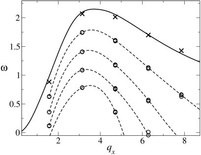
Figure 3: Top) Dispersion relation of growth rate $\omega$ versus wavevector $q_{x}$ during the initial stage of 2D instability, starting with a 1D shear banded planar Poiseuille basic state. In each case $a=0.3$, $\eta=0.05$, $G=4.0$. Circles: extracted from early time dynamics of the full nonlinear code. Groups of data upward correspond to $l=0.02$, 0.015, 0.01, 0.005. Within each group, data are shown for $(Dt,N_{x},N_{y})=(0.000025,200,400)$, (0.0000125, 200, 400), (0.000025, 400, 800). These are mostly indistinguishable, demonstrating convergence with respect to grid and timestep. Dashed lines: cubic splines through the data for $(Dt,N_{x},N_{y})=(0.000025,200,400)$, as a guide to the eye. $L_{x}=4.0$ in each case. Solid line: results of analytical calculation in the true limit $l\to 0$. Crosses: extrapolation of the $l\neq 0$ results to $l=0$ using the scaling $\omega(q_{x},l)=\omega(q_{x},l=0)-a(q_{x})l$.
Bottom) Growth rate (left) and wavevector (right) at the peak of dispersion relations as a function of the pressure drop $G$, calculated analytically in the limit $l\to 0$.

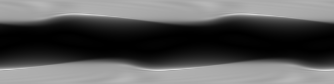
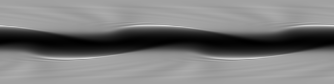
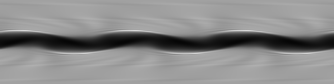
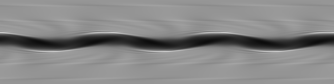
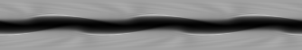
Figure 4: Greyscale snapshots of the order parameter $\Sigma_{xx}(x,y)$ at a representative time $t=60.0$ on the ultimate nonlinear attractor for $a=0.3$, $\eta=0.05$, $l=0.005$ for $L_{x}=4.0$ and $G=2.0$, 4.0, 6.0, 8.0 (top four subfigures downwards) with $Dt=0.000025$, $N_{x}=200$, $N_{y}=400$. Bottom subfigure is for $G=4.0$ with a longer cell $L_{x}=6.0$ (so $N_{x}=300$).

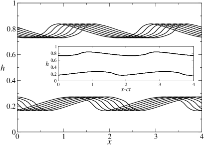
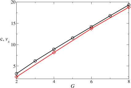
Figure 5: Top) Snapshot of interface height $h(x)$ for $a=0.3$, $\eta=0.05$, $l=0.005$, $L_{x}=4.0$ and $G=2.0$ at six times equally spaced by $\Delta t=0.05265$. $Dt=0.000025$, $N_{x}=200$, $N_{y}=400$. Inset: the same data plotted versus transformed coordinate $x-ct$ revealing simple convective motion with a constant wavespeed $c$.
Bottom) Diamonds: wavespeed $c$ versus pressure drop $G$, obtained by performing the transformation shown in Fig. 5. $a=0.3$, $\eta=0.05$, $l=0.005$, $L_{x}=4.0$ for runs with $Dt=0.000025$, $N_{x}=200$, $N_{y}=400$. Circles: fluid velocity $v_{x}$ at interface, taken from the 1D banded profiles of Fig. 2.

In steady 1D PPF driven by a pressure drop $\partial_{x}P=-G$, Eqn. 1 dictates the shear stress to be linear across the flow cell: $T_{xy}=-G(y-\tfrac{1}{2})$. Well away from any interfaces (the almost vertical regions in Fig. 2, right) the value of the shear rate $\dot{\gamma}$ then follows as the lower (resp. upper) solution branch of the same relation $T_{xy}(\dot{\gamma})=\Sigma_{xy}(\dot{\gamma})+\eta\dot{\gamma}$ discussed above for PCF, in the regions where $|T_{xy}|<T_{\rm sel}$ (resp. $|T_{xy}|>T_{\rm sel}$). This leads to the steady flow states shown in Fig. 2, which are shear banded for all values of the applied pressure drop $G>2T_{\rm sel}$ shown. In bulk rheology, the signature of the transition to shear banded flow is the pronounced kink seen in the composite flow curve of Fig. 1 (right).

The 1D shear banded flows discussed in this section will form the basic states and initial conditions for the stability studies of the rest of the paper. In Sec. IV we will consider 2D flow in the $x$-$y$ plane, with periodic boundaries in the flow direction $x$, and assuming translational invariance in $z$. In Sec. V we will turn to 2D flow in the $y$-$z$ plane, with periodic boundaries in the vorticity direction $z$, and assuming translational invariance in $x$.

IV Flow, flow-gradient plane

In this section we relax the assumption of translational invariance in the flow direction $x$ and perform a two-dimensional study in the flow/flow-gradient ($x$-$y$) plane. As before we consider flow between closed walls at $y=\{0,L_{y}\}$, driven by a constant pressure drop $\partial_{x}p=-G$. The boundaries in $x$ are taken to be periodic. For simplicity, translational invariance is still assumed in the vorticity direction $z$.

Our study comprises two parts. In Sec. IV.1 we study the linear stability of the 1D shear banded basic states of Fig. 2 with respect to perturbations that have infinitesimal amplitude and a wavevector $q_{x}\hat{\mathbf{{x}}}$ in the flow direction. We will show these basic states to be linearly unstable to such perturbations in most regimes. An initial condition comprising shear banded flow with a flat interface is thereby predicted to evolve towards a 2D state that has modulations along the interface, via the growth of these perturbations. In Sec. IV.2 we study the model’s full nonlinear dynamics in this $x$-$y$ plane, giving results for the ultimate 2D flow state that is attained once these modulations have grown to, and (as we shall demonstrate) saturated at, a finite amplitude.

Before presenting our results we discuss briefly our numerical method. In previous work the full nonlinear dynamics of the DJS model in boundary driven PCF were simulated by SMF in the flow/flow-gradient plane fielding-prl-96–2006 , assuming translational invariance in the vorticity direction. During the course of that study, the code was carefully checked against an earlier calculation of the linear stability of an interface between shear bands in PCF fielding-prl-95–2005 ; wilson-jnfm-138-181-2006 , providing a stringent check that the nonlinear code was working correctly. A straightforward two-line modification adapts that code to the pressure driven PPF of interest here.

IV.1 Linear stability analysis

In each run of this modified code we start with an initial condition comprising a 1D banded state of Sec. III, corresponding to shear banded flow with a flat interface between the bands. To this state we add 2D perturbations of tiny amplitude. By monitoring, in this fully nonlinear code, the early-time growth of the Fourier components $\exp(iq_{x}x)\exp(\omega t)$ of the perturbation, we can extract the dispersion relation $\omega(q_{x})$ that characterises the linear instability of the 1D basic state. These numerical results for this dispersion relation are shown by dashed lines in Fig. 3 (top), for different values of the interfacial thickness $l$. As can be seen, at any fixed value of $q_{x}$ the growth rate shows a linear dependence on $l$: $\omega^{*}(l,q_{x})=\omega^{*}(l=0,q_{x})-a(q_{x})l$ where the intercept $\omega^{*}(l=0,q_{x})$ plotted versus $q_{x}$ accordingly forms the dispersion relation extrapolated to $l=0$, shown by the crosses in Fig. 3 (top). The value $l=0$ cannot be accessed in this full nonlinear code, because this limit is pathological in shear banding fluids. However, analytical linear stability calculations can nonetheless still be performed in this limit wilson-jnfm-138-181-2006 . The solid line in Fig. 3 (top) accordingly shows the results of a truly linear analytical stability calculation, performed by HJW in the true limit $l\to 0$. As can be seen, this indeed agrees well with the extrapolation of the numerical results to $l=0$. Because the $l\neq 0$ and $l=0$ calculations were performed independently by the two authors, and using different methods, this provides a good cross check between both sets of results.

Because of the linear nature of this stability system, any eigenvector can be separated into sinuous and varicose contributions, in which the perturbation to the flow field across the channel is odd (snake-like) and even (sausage-like) respectively. Each of these is an eigenvector in its own right. In the $l=0$ calculations, this separation is carried out explicitly. We find that the sinuous (snakelike) modes are always more unstable than varicose ones. Because our interest is in the most unstable mode, the $l=0$ results presented here are all for sinuous perturbations. (In our runs of the full code for $l\not=0$, we do not impose any such symmetry a priori. Instead, it emerges naturally from the full system.)

The location of the peak in the dispersion relation is shown as a function of pressure drop $G$ in Fig. 3 (bottom), for the $l=0$ calculation. As can be seen, for values of $G$ well within the banding regime the growth rate $\omega=O(1)$, comparable to the linear viscoelastic relaxation time, and the wavelength $\lambda_{x}=2\pi/q_{x}=O(2)$, comparable to twice the gap width. This is consistent with the presence of secondary velocity rolls lerouge2008 ; fardin2009 of a wavelength comparable to the gap width, and also consistent with the dominant wavelength seen in our nonlinear results discussed in Fig. 4 below. (Such velocity rolls will be shown explicitly in our corresponding study of the flow-gradient/vorticity plane in Fig. 7 below.) As the applied shear rate approaches the low shear branch from above, and the width of the high shear bands accordingly tends to zero, the growth rate and wavelength of the most unstable perturbations also tend to zero.

For a small range of pressure drops $1.20<G<1.52$, two peaks are evident in the dispersion relation (not shown). For $G\leq 1.3$ the peak with the larger value of $q_{x}$ is the more unstable, with crossover to dominance of the lower $q_{z}$ peak for $G\geq 1.32$. This causes a “kink” in the plot of $\omega^{*}$ against $G$ at $G\approx 1.3$, only just discernible in Fig. 3.

IV.2 Ultimate nonlinear dynamics

At long times the instability described above saturates at the level of finite amplitude undulations along the interface. Representative greyscale snapshots of the system’s eventual state are shown in Fig. 4. As can seen in Fig. 5 (top), the interfacial undulations convect along the positive $x$ direction with constant speed. This speed is plotted as a function of pressure drop in Fig. 5 (bottom), and is comparable, but not exactly equal, to the value of the fluid velocity at the interface. As noted above, our $l\neq 0$ code does not impose any sinuous/varicose symmetry. Indeed, the ultimate nonlinear attractor can be seen in Fig. 4 to be dominated by a mode that is neither fully sinuous not fully varicose.

V Flow-gradient, vorticity plane

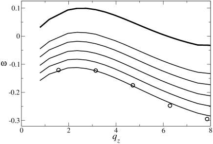
Figure 6: Top) Dispersion relation of growth rate $\omega$ versus wavevector $q_{z}$ during the initial stage of 2D instability, starting with a 1D shear banded planar Poiseuille basic state. In each case $a=0.3$, $\eta=0.05$, $G=4.0$. Thin solid lines: calculated by linear stability analysis using the method of Ref. fielding2007b , with lines upward corresponding to $l=0.0035$, 0.003, 0.0025, 0.002, 0.0015. Thick solid lines: extrapolation of the $l\neq 0$ results shown by each of the thin solid lines to $l=0$ using the scaling $\omega(q_{x},l)=\omega(q_{x},l=0)-a(q_{x})l$. Indistinguishability of the thick lines demonstrates the validity of this scaling. Circles: extracted from early time dynamics of the full nonlinear code for $l=0.0035$.
Bottom) Growth rate (left) and wavevector (right) at the peak of dispersion relation as a function of the pressure drop $G$ for $l=0.003$, 0.0025, 0.002, 0.0015 (sets upwards in left hand figure).

In this section we turn attention to the flow-gradient/vorticity ($y$-$z$) plane, now assuming translational invariance in the flow direction $x$. As usual we assume closed walls in $y$, and (for simplicity) periodic boundaries in $z$. We will return in the conclusion to discuss briefly the implications of having focused only on 2D studies in this paper.

V.1 Linear stability analysis

We consider first the linear stability properties of the 1D basic states of Fig. 2 with respect to fluctuations with wavevector in the vorticity direction, $\exp(iq_{z}z+\omega t)$. To do so we perform a truly linear calculation, calculating the eigenmodes of the stability matrix that is obtained by linearising the full nonlinear equations about the basic state. This linearisation problem was in fact studied previously in the flow-gradient/vorticity plane in the context of planar Couette flow in Ref. fielding2007b . The same linearised code can be used here, simply inserting the new pressure driven basic state as an input to the elements of the matrix.

The resulting dispersion relations $\omega(q_{z})$ are shown in Fig. 6 (top). As is evident, at each value of $q_{z}$ the growth rate increases linearly with decreasing values of the interfacial width $l$, allowing us to extrapolate to the case $l=0$ (thick line in Fig. 6, top), as in the case of the $x$-$y$ plane above. The location $\omega^{*},k^{*}$ of the peak in the dispersion relations is plotted as a function of the pressure drop $G$ in Fig. 6, bottom. As can be seen, for large values of the interfacial width $l$ the instability is absent (all $\omega^{*}<0$). For intermediate values of $l$ there is a window in $G$ between the onset of shear banding and the onset of this interfacial instability. The size of this window decreases with decreasing $l$, and we believe would extrapolate to zero as $l\to 0$, such that all shear banded states are linearly unstable in the limit of a thin interface.

These truly linear results were checked for consistency against the linearised dynamics of a fully nonlinear code, which directly simulates the full 2D dynamics of the model in the $yz$ plane. (The main use of this code is to generate the results in the next subsection.) In each run of this nonlinear code we used as an initial condition the 1D basic state of Fig. 2, subject to small 2D fluctuations in the $y$-$z$ plane. By monitoring the early-time growth of the Fourier components $\exp(iq_{z}z)\exp(\omega t)$ we extracted the dispersion relation $\omega(q_{z})$ for the linear (in)stability of the 1D basic state. As shown by the circles in Fig. 6, good agreement is found with the true linear stability calculation described in the previous paragraph. This provides a stringent cross check between our linear stability calculation and our nonlinear code.

V.2 Ultimate nonlinear attractor

In previous work we simulated the full nonlinear dynamics of the DJS model in 2D plane Couette flow in the flow-gradient/ vorticity ($y$-$z$) plane fielding2007b , assuming translational invariance in the flow direction $x$. A straightforward two-line modification allows this code to be adapted to the case of pressure driven flow of interest here. As described in the previous section, we performed a series of runs of this code starting with a 1D basic state, subject to small 2D perturbations. We consider in this section the ultimate state that the system attains at long times. In each case, the instability was found to saturate in a steady state with finite amplitude undulations along the interface (Fig. 7, top). Such undulations have recently been imaged experimentally in the pressure driven flow of wormlike micelles in microchannels of high aspect ratio submitted . Associated with these undulations is a secondary flow comprising the velocity rolls shown in the second subfigure (Fig. 7, bottom).

Figure 7: Order parameter $\Sigma_{xx}(y,z)$ greyscale (top) and velocity map showing secondary flow in $y$-$z$ plane (bottom): snapshot at time $t=1895$ in steady state for $a=0.3$, $\eta=0.05$, $l=0.0015$ for $L_{x}=4.0$ and $G=2.0$ with $Dt=0.05$, $N_{z}=1000$, $N_{y}=1066$.

VI Summary and outlook

In this work, we have studied the pressure driven planar Poiseuille flow of a shear banding fluid sandwiched between infinite stationary flat parallel plates. Using a combination of linear stability analysis and direct numerical simulation, we have shown an initially flat interface between shear bands to be unstable with respect to the growth of undulations along it. The early time growth rate of these undulations scales as the reciprocal stress relaxation time of the fluid, and the corresponding wavelength is comparable to the separation of the plates. At long times the undulations saturate in a finite amplitude, cutoff by the nonlinear effects of shear.

Throughout our study we have neglected any in-flow and out-flow effects at the start and end of the channel, assuming a well established flow field that is free from end effects. Associated with this is our assumption that the spatial limits relevant to this established flow field correspond to the temporal limit $t\to\infty$ in each run of our code. We have furthermore neglected the effect of any lateral walls in the $z$ direction, taking from the outset the limit $L_{z}/L_{y}\to\infty$. In practice one might expect lateral walls to impose a further loss of translational symmetry in the $z$ direction, as explored in Ref. submitted . Perhaps most importantly, in conducting separate two-dimensional studies in the $x-y$ and $y-z$ planes, we have neglected the possibility that exists in three spatial dimensions of nonlinear interactions between the $q_{x}$ and $q_{z}$ modes. Indeed, although the $q_{x}$ modes have much faster growth rates than the $q_{z}$ modes in the early time (linear) growth regime, they are cut off more aggressively at nonlinear order by the effects of shear. This results in comparable amplitudes for the $q_{x}$ and $q_{z}$ models in the ultimate attractors of our separate 2D studies. It therefore seems unlikely that 3D effects cannot be neglected, as we shall explore in future. We mention finally that the constitutive model used in the present work is highly oversimplified, in particular in having a Newtonian high shear branch.

Recent experiments in microchannel flow used 1D velocimetry imaging to reconstruct the local flow curves of a shear banding wormlike micellar surfactant solution masselon2008 . Surprisingly, these curves were found to be non-universal, failing to collapse when plotted for different applied pressure gradients on a single plot. Possible explanations of this observation, to be explored in future work, include: a larger ratio $l/L_{y}$ than considered here; coupling between flow and concentration; and the effects of secondary 3D flows.

VII Acknowledgements

SMF thanks Tony Maggs for his hospitality during a research visit, funded by the CNRS of France, to the Laboratoire de Physico-Chimie Théorique (PCT) at ESPCI in Paris, where this work was partly carried out. SMF also thanks Philippe Nghe and Patrick Tabeling in the Microfluidique, MEMS et Nanostructures group at ESPCI, and Armand Ajdari of PCT for stimulating discussions. Financial support for SMF is acknowledged from the UK’s EPSRC in the form of an Advanced Research Fellowship, grant reference EP/E5336X/1.

References

- (1) N. A. Spenley, M. E. Cates, and T. C. B. McLeish, Phys. Rev. Lett. 71, 939 (1993).
- (2) N. A. Spenley, X. F. Yuan, and M. E. Cates, J. Phys. II (France) 6, 551 (1996).
- (3) J. Yerushalmi, S. Katz, and R. Shinnar, Chemical Engineering Science 25, 1891 (1970).
- (4) H. Rehage and H. Hoffmann, Mol. Phys. 74, 933 (1991).
- (5) J. P. Decruppe, R. Cressely, R. Makhloufi, and E. Cappelaere, Coll. Polym. Sci. 273, 346 (1995).
- (6) M. M. Britton and P. T. Callaghan, Phys. Rev. Lett. 78, 4930 (1997).
- (7) P. Callaghan, Rheologica Acta 47, 243 (2008).
- (8) L. Becu, S. Manneville, and A. Colin, Phys. Rev. Lett. 93, art. no. (2004).
- (9) S. Manneville, Rheologica Acta 47, 301 (2008).
- (10) J. B. Salmon, A. Colin, S. Manneville, and F. Molino, Phys. Rev. Lett. 90, art. no. (2003).
- (11) Y. T. Hu and A. Lips, J. Rheology 49, 1001 (2005).
- (12) J. F. Berret, D. C. Roux, and G. Porte, J. Phys. II (France) 4, 1261 (1994).
- (13) P. T. Callaghan, M. E. Cates, C. J. Rofe, and J. A. F. Smeulders, J. Phys. II (France) 6, 375 (1996).
- (14) C. Grand, J. Arrault, and M. E. Cates, J. Phys. II (France) 7, 1071 (1997).
- (15) J. F. Berret, D. C. Roux, G. Porte, and P. Lindner, Europhys. Lett. 25, 521 (1994).
- (16) V. Schmitt, F. Lequeux, A. Pousse, and D. Roux, Langmuir 10, 955 (1994).
- (17) E. Cappelaere et al., Phys. Rev. E 56, 1869 (1997).
- (18) R. Makhloufi, J. P. Decruppe, A. Aitali, and R. Cressely, Europhys. Lett. 32, 253 (1995).
- (19) J. F. Berret, G. Porte, and J. P. Decruppe, Phys. Rev. E 55, 1668 (1997).
- (20) O. Diat, D. Roux, and F. Nallet, J. Phys. II (France) 3, 1427 (1993).
- (21) G. M. H. Wilkins and P. D. Olmsted, European Physical Journal E 21, 133 (2006).
- (22) D. Bonn et al., Phys. Rev. E 58, 2115 (1998).
- (23) J. B. Salmon, S. Manneville, and A. Colin, Phys. Rev. E 68, art. no. (2003).
- (24) J. B. Salmon, S. Manneville, and A. Colin, Phys. Rev. E 68, art. no. (2003).
- (25) S. Manneville, J. B. Salmon, and A. Colin, Eur. Phys. J. E 13, 197 (2004).
- (26) C. Pujolle-Robic and L. Noirez, Nature 409, 167 (2001).
- (27) M. P. Lettinga and J. K. G. Dhont, J. Physics-condensed Matter 16, S3929 (2004).
- (28) J. K. G. Dhont and W. J. Briels, J. Chem. Phys. 118, 1466 (2003).
- (29) J. F. Berret and Y. Serero, Phys. Rev. Lett. 8704, (2001).
- (30) P. Coussot et al., Phys. Rev. Lett. 88, art. no. (2002).
- (31) W. M. Holmes, P. T. Callaghan, D. Vlassopoulos, and J. Roovers, J. Rheology 48, 1085 (2004).
- (32) S. Rogers, D. Vlassopoulos, and P. Callaghan, Physical Review Letters 100, 128304 (2008).
- (33) L. Hilliou and D. Vlassopoulos, Ind. Eng. Chem. Res. 41, 6246 (2002).
- (34) L. B. Chen et al., Phys. Rev. Lett. 69, 688 (1992).
- (35) W. M. Holmes, M. R. Lopez-Gonzalez, and P. T. Callaghan, Europhysics Lett. 64, 274 (2003).
- (36) M. R. Lopez-Gonzalez, W. M. Holmes, P. T. Callaghan, and P. J. Photinos, Phys. Rev. Lett. 93, (2004).
- (37) R. Bandyopadhyay, G. Basappa, and A. K. Sood, Phys. Rev. Lett. 84, 2022 (2000).
- (38) R. Ganapathy and A. K. Sood, Phys. Rev. Lett. 96, (2006).
- (39) Y. T. Hu, P. Boltenhagen, and D. J. Pine, J. Rheol. 42, 1185 (1998).
- (40) R. Bandyopadhyay and A. K. Sood, Europhysics Lett. 56, 447 (2001).
- (41) E. K. Wheeler, P. Fischer, and G. G. Fuller, J. Non-newtonian Fluid Mechanics 75, 193 (1998).
- (42) V. Herle, P. Fischer, and E. J. Windhab, Langmuir 21, 9051 (2005).
- (43) P. Fischer, Rheologica Acta 39, 234 (2000).
- (44) H. Azzouzi, J. P. Decruppe, S. Lerouge, and O. Greffier, European Phys. J. E 17, 507 (2005).
- (45) J. P. Decruppe, O. Greffier, S. Manneville, and S. Lerouge, Phys. Rev. E 73, (2006).
- (46) J.-B. Salmon, A. Colin, and D. Roux, Phys. Rev. E 66, art. no. (2002).
- (47) S. Lerouge, M. Argentina, and J. P. Decruppe, Phys. Rev. Lett. 96, (2006).
- (48) S. Lerouge et al., Soft Matter 4, 1808 (2008).
- (49) M. Fardin et al., Physical Review Letters 103, 028302 (2009).
- (50) S. M. Fielding, Phys. Rev. Lett. 95, (2005).
- (51) H. J. Wilson and S. M. Fielding, J. Non-newtonian Fluid Mechanics 138, 181 (2006).
- (52) S. Fielding, Physical Review E 76, 016311 (2007).
- (53) E. J. Hinch, O. J. Harris, and J. M. Rallison, J. Non-newtonian Fluid Mechanics 43, 311 (1992).
- (54) R. G. Larson, E. S. G. Shaqfeh, and S. J. Muller, J. Fluid Mechanics 218, 573 (1990).
- (55) P. Nghe, G. Degre, P. Tabeling, and A. Ajdari, Applied Physics Letters 93, (2008).
- (56) C. Masselon, J. Salmon, and A. Colin, Physical Review Letters 100, 038301 (2008).
- (57) P. Nghe, S. M. Fielding, P. Tabeling, and A. Ajdari, Submitted for publication (2009).
- (58) M. W. Johnson and D. Segalman, J. Non-newtonian Fluid Mechanics 2, 255 (1977).
- (59) P. D. Olmsted, O. Radulescu, and C. Y. D. Lu, J. Rheology 44, 257 (2000).
- (60) C. Y. D. Lu, P. D. Olmsted, and R. C. Ball, Phys. Rev. Lett. 84, 642 (2000).
- (61) J. Adams, S. Fielding, and P. Olmsted, Journal Of Non-Newtonian Fluid Mechanics 151, 101 (2008).
- (62) S. M. Fielding and P. D. Olmsted, European Phys. J. E 11, 65 (2003).
- (63) S. M. Fielding and P. D. Olmsted, Phys. Rev. Lett. 96, (2006).