$\mathcal{N}=4$ Superconformal Algebra and the Entropy of HyperKähler Manifolds

Abstract.

We study the elliptic genera of hyperKähler manifolds using the representation theory of $\mathcal{N}=4$ superconformal algebra. We consider the decomposition of the elliptic genera in terms of $\mathcal{N}=4$ irreducible characters, and derive the rate of increase of the multiplicities of half-BPS representations making use of Rademacher expansion. Exponential increase of the multiplicity suggests that we can associate the notion of an entropy to the geometry of hyperKähler manifolds. In the case of symmetric products of $K3$ surfaces our entropy agrees with the black hole entropy of D5-D1 system.

1. Introduction

It has been known for some time  [18] that characters of the BPS representations of the extended superconformal algebra do not in general have a good modular property. This is because of the existence of special singular vectors coming from the BPS condition ($G^{i}|h\rangle=0$). Thus BPS characters are not regular theta functions but are mock (pseudo) theta functions of the kind first introduced by Ramanujan [1, 9]. Systematic understanding of mock theta functions, however, was not available until very recently. Intrinsic structure behind them was first revealed by Zwegers several years ago  [48], and they are identified as the holomorphic part of the harmonic Maass forms (see Appendix for definition). Since the work of Zwegers, the theory of the mock theta function has been applied to the theory of partitions [2], and its relationship with the quantum invariant for links and 3-manifolds has been clarified  [31, 27, 24, 23, 25, 26, 46] (see Ref. 37 for a review on recent developments).

This paper is a sequel to our previous papers [10, 11], where we have studied representation theory of the $\mathcal{N}=4$ superconformal algebras using the method of Zwegers and in particular the decomposition of the elliptic genus of the $K3$ surface in terms of irreducible characters of $\mathcal{N}=4$ algebra.

In general the elliptic genus of hyperKähler manifold of complex-dimension $2k$ has an expansion

$$\mbox{elliptic genus}=\sum_{\ell\in\left\{0,\frac{1}{2},\dots,{k\over 2}\right\}}c_{\ell}\,\left[\mbox{BPS representation}:h={k\over 4},\ell\right]\\ +\sum_{n=1}^{\infty}\sum_{\ell\in\left\{{1\over 2},1,\dots,{k\over 2}\right\}}p_{k}^{(\ell)}(n)\,\left[\mbox{non-BPS representation}:h=n+{k\over 4},\ell\right].$$ (1.1)

Here $h$ and $\ell$ respectively denote the conformal dimension and isospin of highest weight states. In this paper we introduce the Rademacher expansion and determine the asymptotic behavior of the multiplicity factors $p_{k}^{(\ell)}(n)$ as $n$ becomes large. We shall show that they have an exponential growth and at large $k$ behave as

$$p_{k}^{(\ell)}(n)\sim\exp\left(2\,\pi\,\sqrt{k\,n-\ell^{2}}\right).$$ (1.2)

Such an exponential behavior of the degeneracy is reminiscent of the entropy of black holes.

In the elliptic genus the right-moving sector is held fixed at the Ramond ground state and hence the non-BPS states in (1.1) are actually the half-BPS states (BPS (non-BPS) in the right-(left-)moving sector). Counting the asymptotic degeneracy of states protected by supersymmetry amounts to computing the entropy of systems. Actually as we see below, when one considers the case of symmetric product of $K3$ surfaces $K3^{[k]}$ it in fact agrees with the entropy of the standard D5-D1 black holes in $AdS^{3}\times S^{3}\times K3$ [42, 6]. Positivity inside the square root of (1.2) corresponds to the cosmic censorship in classical general relativity [6, 7].

We propose in this paper that arbitrary hyperKähler manifolds carry entropy as defined above. In (1.1) a bad modular property of BPS characters is exactly compensated by the equally bad modular property of the infinite series $\sum_{n}p_{k}^{(\ell)}(n)\,q^{n}$. Thus the lack of modular behavior of BPS characters is the origin of entropy in hyperKähler manifolds.

This paper is organized as follows. In Section 2 we briefly review our previous results in Refs. 10, 11. In Section 3 we study the Rademacher expansion of the Fourier coefficients of the vector-valued harmonic Maass form by use of the Poincaré–Maass series. In Section 4 we study the decomposition of the elliptic genera of the hyperKähler manifolds in terms of irreducible characters. By use of the Rademacher expansion, we derive the asymptotic behavior of the multiplicity of the non-BPS representations. We present the cases of level-$2$ and -$3$ in some detail. The last section contains concluding remarks.

2. Superconformal Algebras and Mock Theta Functions

2.1. Characters of Superconformal Algebras

The $\mathcal{N}=4$ superconformal algebra at level $k$ has a central charge $c=6\,k$, and contains an affine $SU(2)_{k}$ algebra. Its highest weight state $|\Omega\rangle$ is labeled by the conformal weight $h$ and the isospin $\ell$,

$$\begin{gathered}L_{0}\,|\Omega\rangle=h\,|\Omega\rangle,\\ T_{0}^{3}\,|\Omega\rangle=\ell\,|\Omega\rangle.\end{gathered}$$

The character of a representation is defined by

$$\operatorname{ch}_{k,h,\ell}(z;\tau)=\operatorname{Tr}_{\mathcal{H}}\left(\mathrm{e}^{4\,\pi\,\mathrm{i}\,z\,T_{0}^{3}}\,q^{L_{0}-\frac{c}{24}}\right),$$ (2.1)

where $q=\mathrm{e}^{2\,\pi\,\mathrm{i}\,\tau}$ with $\tau\in\mathbb{H}$, and $\mathcal{H}$ denotes the Hilbert space of the representation. In the following we often use $\zeta=\mathrm{e}^{2\,\pi\,\mathrm{i}\,z}$ with $z\in\mathbb{C}$. In $\mathcal{N}=4$ theory we have two types of representations [16, 17, 18]; massless (BPS) and massive (non-BPS) representations. In the Ramond sector, their character formulas are given as follows;

• massless representations ($h=\frac{k}{4}$, and $\ell=0,\frac{1}{2},\dots,\frac{k}{2}$),

  $$\operatorname{ch}^{R}_{k,\frac{k}{4},\ell}(z;\tau)=\frac{\mathrm{i}}{\theta_{11}(2z;\tau)}\cdot\frac{\left[\theta_{10}(z;\tau)\right]^{2}}{\left[\eta(\tau)\right]^{3}}\sum_{\varepsilon=\pm 1}\sum_{m\in\mathbb{Z}}\varepsilon\,\frac{\mathrm{e}^{4\pi\mathrm{i}\varepsilon\left((k+1)m+\ell\right)z}}{\left(1+\mathrm{e}^{-2\pi\mathrm{i}\varepsilon z}\,q^{-m}\right)^{2}}\,q^{(k+1)\,m^{2}+2\,\ell\,m},$$ (2.2)

• massive representations ($h>\frac{k}{4}$ and $\ell=\frac{1}{2},1,\dots,\frac{k}{2}$),

  $$\operatorname{ch}^{R}_{k,h,\ell}(z;\tau)=q^{h-\frac{\ell^{2}}{k+1}-\frac{k}{4}}\,\frac{\left[\theta_{10}(z;\tau)\right]^{2}}{\left[\eta(\tau)\right]^{3}}\,\chi_{k-1,\ell-\frac{1}{2}}(z;\tau),$$ (2.3)

  where $\chi_{k,\ell}(z;\tau)$ denotes the affine SU($2$) character

  $$\chi_{k,\ell}(z;\tau)=\frac{\vartheta_{k+2,2\ell+1}-\vartheta_{k+2,-2\ell-1}}{\vartheta_{2,1}-\vartheta_{2,-1}}(z;\tau),$$ (2.4)

  with the theta series defined by

  $$\vartheta_{P,a}(z;\tau) =\sum_{n\in\mathbb{Z}}q^{\frac{(2Pn+a)^{2}}{4P}}\,\mathrm{e}^{2\pi\mathrm{i}z(2Pn+a)}.$$ (2.5)

  Note that the denominator of the affine character equals

  $$\left(\vartheta_{2,1}-\vartheta_{2,-1}\right)(z;\tau)=-\mathrm{i}\,\theta_{11}(2\,z;\tau).$$ (2.6)

Characters in other sectors are obtained by spectral flow: $z\rightarrow z+{1\over 2}\,(\widetilde{R})$, $z\rightarrow z+{\tau\over 2}\,(NS)$, $z\rightarrow z+{1+\tau\over 2}\,(\widetilde{NS})$.

At the unitarity boundary $h=\frac{k}{4}$, the non-BPS representation decomposes into a sum of the BPS representations. For instance, in the $\widetilde{R}$ sector ($R$ sector with $(-1)^{F}$ insertion) we have

$$\lim_{h\searrow\frac{k}{4}}\operatorname{ch}^{\widetilde{R}}_{k,h,\ell}(z;\tau) =(-1)^{2\ell+1}\,q^{-\frac{\ell^{2}}{k+1}}\,\frac{\left[\theta_{11}(z;\tau)\right]^{2}}{\left[\eta(\tau)\right]^{3}}\,\chi_{k-1,\ell-\frac{1}{2}}(z;\tau)$$ (2.7)

$$=\operatorname{ch}^{\widetilde{R}}_{k,\frac{k}{4},\ell}(z;\tau)+2\,\operatorname{ch}^{\widetilde{R}}_{k,\frac{k}{4},\ell-\frac{1}{2}}(z;\tau)+\operatorname{ch}^{\widetilde{R}}_{k,\frac{k}{4},\ell-1}(z;\tau).$$

2.2. Conformal Characters and Mock Theta Functions

For notational convenience we set the holomorphic function $C_{k}(z;\tau)$ to be the massless superconformal character with isospin-$0$ in $\widetilde{R}$ sector; 

$$C_{k}(z;\tau) =\operatorname{ch}_{k,h=\frac{k}{4},\ell=0}^{\widetilde{R}}(z;\tau)$$

$$=\frac{\left[\theta_{11}(z;\tau)\right]^{2}}{\left[\eta(\tau)\right]^{3}}\,\frac{\mathrm{i}}{\theta_{11}(2\,z;\tau)}\,\sum_{n\in\mathbb{Z}}q^{(k+1)\,n^{2}}\,\mathrm{e}^{4\pi\mathrm{i}(k+1)nz}\,\frac{1+q^{n}\,\mathrm{e}^{2\pi\mathrm{i}z}}{1-q^{n}\,\mathrm{e}^{2\pi\mathrm{i}z}}.$$ (2.8)

Note that massless representation carries the Witten index

$$C_{k}(z=0;\tau)=1.$$ (2.9)

It is known that the function $C_{k}(z;\tau)$ does not have a good behavior under modular transformation: one has to find its suitable “completion” which has a good modular behavior. The following completion of $C_{k}(z;\tau)$ has been obtained in our previous work  [10]

$$\widehat{C}_{k}(z;\tau)=C_{k}(z;\tau)-\frac{1}{\mathrm{i}\sqrt{2\,(k+1)}}\,\sum_{a=1}^{k}R_{k}^{(a)}(\tau)\,B_{k}^{(a)}(z;\tau).$$ (2.10)

Here the basis functions $B_{k}^{(a)}(z;\tau)$ are proportional to the massive characters of $\mathcal{N}=4$ algebra (2.3)

$$B_{k}^{(a)}(z;\tau) =\frac{\left[\theta_{11}(z;\tau)\right]^{2}}{\left[\eta(\tau)\right]^{3}}\,\chi_{k-1,\frac{a-1}{2}}(z;\tau)$$

$$=\frac{\left[\theta_{11}(z;\tau)\right]^{2}}{\left[\eta(\tau)\right]^{3}}\cdot\frac{\vartheta_{k+1,a}-\vartheta_{k+1,-a}}{\vartheta_{2,1}-\vartheta_{2,-1}}(z;\tau).$$ (2.11)

The non-holomorphic function $R_{k}^{(a)}(\tau)$ is defined as

$$R_{k}^{(a)}(\tau)=\mathrm{i}\sqrt{2\,(k+1)}\sum_{\begin{subarray}{c}n\in\mathbb{Z}\\ n=a\mod 2(k+1)\end{subarray}}\left[\operatorname{sgn}\left(n+\frac{1}{2}\right)-E\left(n\,\sqrt{\frac{\Im\tau}{k+1}}\right)\right]\,q^{-\frac{n^{2}}{2(k+1)}},$$ (2.12)

where $E(x)$ is the error function

$$E(x)=2\int_{0}^{x}\mathrm{e}^{-\pi\,t^{2}}\,\mathrm{d}t=1-\operatorname{erfc}\left(\sqrt{\pi}\,x\right).$$

The function $R_{k}^{(a)}(\tau)$ can be rewritten as a period integral,

$$R_{k}^{(a)}(\tau)=\int_{-\overline{\tau}}^{\mathrm{i}\infty}\frac{\Psi_{k}^{(a)}(z)}{\sqrt{\frac{z+\tau}{\mathrm{i}}}}\,\mathrm{d}z,$$ (2.13)

where $\Psi_{k}^{(a)}(\tau)$ denotes a vector-valued modular form with weight-$3/2$ proportional to the affine SU(2) character;

$$\Psi_{k}^{(a)}(\tau)=\left[\eta(\tau)\right]^{3}\chi_{k-1,\frac{a-1}{2}}(0;\tau)=\left[\eta(\tau)\right]^{3}\frac{\vartheta_{k+1,a}-\vartheta_{k+1,-a}}{\vartheta_{2,1}-\vartheta_{2,-1}}(0;\tau).$$ (2.14)

In the sense of Zagier [47], the massless superconformal character $C_{k}(z;\tau)$ is a mock theta function whose shadow is $\Psi_{k}^{(a)}(\tau)$. The completion $\widehat{C}_{k}(z;\tau)$ is a real analytic Jacobi form with weight-$0$ and index-$k$. Its modular properties are summarized as follows;

$$\begin{gathered}\widehat{C}_{k}(z;\tau)=\mathrm{e}^{-2\pi\mathrm{i}k\frac{z^{2}}{\tau}}\,\widehat{C}_{k}\left(\frac{z}{\tau};-\frac{1}{\tau}\right),\\[5.69054pt] \widehat{C}_{k}(z;\tau+1)=\widehat{C}_{k}(z+1;\tau)=\widehat{C}_{k}(z;\tau),\\[5.69054pt] \widehat{C}_{k}(z+\tau;\tau)=q^{-k}\,\mathrm{e}^{-4\pi\mathrm{i}kz}\,\widehat{C}_{k}(z;\tau).\end{gathered}$$ (2.15)

We notice that the basis function $B_{k}^{(a)}(z;\tau)$ is a vector-valued Jacobi form with weight-($-1/2$) and index-$k$;

$$\begin{gathered}B_{k}^{(a)}(z;\tau)=-\sqrt{\frac{\tau}{\mathrm{i}}}\,\mathrm{e}^{-2\pi\mathrm{i}k\frac{z^{2}}{\tau}}\,\sum_{b=1}^{k}\sqrt{\frac{2}{k+1}}\,\sin\left(\frac{a\,b}{k+1}\,\pi\right)\,B_{k}^{(b)}\left(\frac{z}{\tau};-\frac{1}{\tau}\right),\\[5.69054pt] B_{k}^{(a)}(z;\tau+1)=\mathrm{e}^{\frac{a^{2}}{2(k+1)}\pi\mathrm{i}}\,B_{k}^{(a)}(z;\tau),\\[5.69054pt] B_{k}^{(a)}(z+1;\tau)=B_{k}^{(a)}(z;\tau),\\[5.69054pt] B_{k}^{(a)}(z+\tau;\tau)=q^{-k}\,\mathrm{e}^{-4\pi\mathrm{i}kz}\,B_{k}^{(a)}(z;\tau).\end{gathered}$$ (2.16)

2.3. Harmonic Maass Form

Next we define the elements of a $k\times k$ matrix $\mathbf{B}_{k}(\boldsymbol{z};\tau)$ as

$$\left(\mathbf{B}_{k}(\boldsymbol{z};\tau)\right)_{ab}=B_{k}^{(b)}(z_{a};\tau),$$ (2.17)

for $1\leq a,b\leq k$, and $z_{a}\in\mathbb{C}$. We introduce  [10]

$$H_{k}^{(a)}(z_{1},\dots,z_{k};\tau)=\sum_{b=1}^{k}\left(\mathbf{B}_{k}(\boldsymbol{z};\tau)^{-1}\right)_{ab}\,C_{k}(z_{b};\tau),$$ (2.18)

whose completion is

$$\widehat{H}_{k}^{(a)}(z_{1},\dots,z_{k};\tau)=\sum_{b=1}^{k}\left(\mathbf{B}_{k}(\boldsymbol{z};\tau)^{-1}\right)_{ab}\,\widehat{C}_{k}(z_{b};\tau).$$ (2.19)

We then have the modular transformation laws,

$$\begin{gathered}\widehat{H}_{k}^{(a)}(z_{1},\dots,z_{k};\tau)=-\sqrt{\frac{\mathrm{i}}{\tau}}\sum_{b=1}^{k}\sqrt{\frac{2}{k+1}}\,\sin\left(\frac{a\,b}{k+1}\,\pi\right)\,\widehat{H}_{k}^{(b)}\left(\frac{z_{1}}{\tau},\dots,\frac{z_{k}}{\tau};-\frac{1}{\tau}\right),\\[5.69054pt] \widehat{H}_{k}^{(a)}(z_{1},\dots,z_{k};\tau+1)=\mathrm{e}^{-\frac{a^{2}}{2(k+1)}\,\pi\,\mathrm{i}}\,\widehat{H}_{k}^{(a)}(z_{1},\dots,z_{k};\tau),\\[5.69054pt] \begin{aligned} \widehat{H}_{k}^{(a)}(z_{1},\dots,z_{b}+1,\dots,z_{k};\tau)&=\widehat{H}_{k}^{(a)}(z_{1},\dots,z_{b}+\tau,\dots,z_{k};\tau)\\ &=\widehat{H}_{k}^{(a)}(z_{1},\dots,z_{k};\tau).\end{aligned}\end{gathered}$$ (2.20)

We note that $\widehat{H}^{(a)}_{k}(z_{i};\tau)$ and $H^{(a)}_{k}(z_{i};\tau)$ are related as

$$\widehat{H}^{(a)}_{k}(z_{1},\cdots,z_{k};\tau)=H^{(a)}_{k}(z_{1},\cdots,z_{k};\tau)-{R^{(a)}_{k}(\tau)\over\mathrm{i}\sqrt{2(k+1)}}.$$ (2.21)

From (2.13) it follows that

$$\frac{\partial}{\partial\overline{\tau}}\,R_{k}^{(a)}(\tau)=\frac{\Psi_{k}^{(a)}(-\overline{\tau})}{\sqrt{2\,\Im\tau}},$$ (2.22)

and we obtain

$$\frac{\partial}{\partial\overline{\tau}}\widehat{H}_{k}^{(a)}(z_{1},\dots,z_{k};\tau)=\frac{\mathrm{i}}{\sqrt{2\,(k+1)}}\,\frac{1}{\sqrt{2\,\Im\tau}}\,\Psi_{k}^{(a)}\left(-\overline{\tau}\right).$$ (2.23)

As a result, the completion $\widehat{H}_{k}^{(a)}(z_{1},\dots,z_{k};\tau)$ is a harmonic Maass form, and is an eigenfunction of the differential operator

$$\Delta_{\frac{1}{2}}\widehat{H}_{k}^{(a)}(z_{1},\dots,z_{k};\tau)=0.$$ (2.24)

Here $\Delta_{\ell}$ denotes the hyperbolic Laplacian ($\tau=u+\mathrm{i}\,v$)

$$\Delta_{\ell} =-v^{2}\,\left(\frac{\partial^{2}}{\partial u^{2}}+\frac{\partial^{2}}{\partial v^{2}}\right)+\mathrm{i}\,{\ell}\,v\,\left(\frac{\partial}{\partial u}+\mathrm{i}\,\frac{\partial}{\partial v}\right)$$

$$=-4\,\left(\Im\tau\right)^{2-\ell}\frac{\partial}{\partial\tau}\left(\Im\tau\right)^{\ell}\frac{\partial}{\partial\overline{\tau}}.$$ (2.25)

Correspondingly, the function $H_{k}^{(a)}(z_{1},\dots,z_{k};\tau)$ defined in (2.18) is regarded as a holomorphic part of the harmonic Maass form.

2.4. Jacobi Form

The Jacobi form $f(z;\tau)$ with weight-$k$ and index-$m$ obeys the following transformation laws [19];

$$\begin{gathered}f\left(\frac{z}{\tau};-\frac{1}{\tau}\right)=\tau^{k}\,\mathrm{e}^{2\pi\mathrm{i}m\frac{z^{2}}{\tau}}\,f(z;\tau),\\[5.69054pt] f(z;\tau+1)=f(z+1;\tau)=f(z;\tau),\\[5.69054pt] f(z+\tau;\tau)=q^{-m}\,\mathrm{e}^{-4\pi\mathrm{i}mz}\,f(z;\tau).\end{gathered}$$ (2.26)

It is known [19] that the space of the Jacobi form with even weight is spanned by

$$\left\{E_{4}(\tau),E_{6}(\tau),\phi_{-2,1}(z;\tau),\phi_{0,1}(z;\tau)\right\},$$

and a basis of Jacobi forms with weight-$k$ and index-$m$ is given by

$$\left[E_{4}(\tau)\right]^{a}\,\left[E_{6}(\tau)\right]^{b}\,\left[\phi_{-2,1}(z;\tau)\right]^{c}\,\left[\phi_{0,1}(z;\tau)\right]^{d},$$ (2.27)

with non-negative integers $a$, $b$, $c$, $d$ satisfying

$$4\,a+6\,b-2\,c=k,\hskip 8.53581ptc+d=m.$$

Here $E_{4}(\tau)$ and $E_{6}(\tau)$ are the Eisenstein series,

$$E_{4}(\tau) =1+240\sum_{n=1}^{\infty}\sigma_{3}(n)\,q^{n}$$

$$=1+240\,q+2160\,q^{2}+6720\,q^{3}+17520\,q^{4}+30240\,q^{5}+\cdots,$$

$$E_{6}(\tau) =1-504\sum_{n=1}^{\infty}\sigma_{5}(n)\,q^{n}$$

$$=1-504\,q-16632\,q^{2}-122976\,q^{3}-532728\,q^{4}-\cdots,$$

where

$$\sigma_{k}(n)=\sum_{r|n}r^{k}.$$

The remaining two functions with index-$1$ are defined by

$${\phi}_{-2,1}(z;\tau) =-\frac{\left[\theta_{11}(z;\tau)\right]^{2}}{\left[\eta(\tau)\right]^{6}}$$ (2.28)

$$=\left(\zeta-2+\zeta^{-1}\right)+\left(-2\,\zeta^{2}+8\,\zeta-12+8\,\zeta^{-1}-2\,\zeta^{-2}\right)\,q$$

$$\quad\qquad+\left(\zeta^{3}-12\,\zeta^{2}+39\,\zeta-56+39\,\zeta^{-1}-12\,\zeta^{-2}+\zeta^{-3}\right)\,q^{2}+\cdots,$$

$${\phi}_{0,1}(z;\tau) =4\,\left[\left(\frac{\theta_{10}(z;\tau)}{\theta_{10}(0;\tau)}\right)^{2}+\left(\frac{\theta_{00}(z;\tau)}{\theta_{00}(0;\tau)}\right)^{2}+\left(\frac{\theta_{01}(z;\tau)}{\theta_{01}(0;\tau)}\right)^{2}\right]$$ (2.29)

$$=\left(\zeta+10+\zeta^{-1}\right)+\left(10\,\zeta^{2}-64\,\zeta+108-64\,\zeta^{-1}+10\,\zeta^{-2}\right)\,q$$

$$\qquad\quad+\left(\zeta^{3}+108\,\zeta^{2}-513\,\zeta+808-513\,\zeta^{-1}+108\,\zeta^{-2}+\zeta^{-3}\right)\,q^{2}+\cdots.$$

It is noted that

$$\phi_{-2,1}(0;\tau) =0,$$ (2.30)

$$\phi_{0,1}(0;\tau) =12,$$

and that $\phi_{0,1}(z;\tau)$ is just one-half of the elliptic genus of the $K3$ surface [13, 30].

2.5. Character Decomposition of Elliptic Genera

In terms of the completion $\widehat{C}_{k}(z;\tau)$ of the massless character and the harmonic Maass form $\widehat{H}^{(a)}_{k}(z_{1},\dots,z_{k};\tau)$, we introduce the function $J_{k}(z;w_{1},\dots,w_{k};\tau)$ as  [10]

$$J_{k}\left(z;w_{1},\dots,w_{k};\tau\right) =\widehat{C}_{k}(z;\tau)-\sum_{a=1}^{k}\widehat{H}_{k}^{(a)}\left(w_{1},\dots,w_{k};\tau\right)\,B_{k}^{(a)}(z;\tau)$$ (2.31)

$$={C}_{k}(z;\tau)-\sum_{a=1}^{k}{H}_{k}^{(a)}\left(w_{1},\dots,w_{k};\tau\right)\,B_{k}^{(a)}(z;\tau).$$ (2.32)

Non-holomorphic dependence in (2.31) cancels each other, and the function $J_{k}(z;w_{1},\dots,w_{k};\tau)$ is holomorphic as is seen in (2.32). $J_{k}(z;w_{1},\dots,w_{k};\tau)$ transforms like a Jacobi form with weight-$0$ and index-$k$ [19];

$$\begin{gathered}J_{k}(z;w_{1},\dots,w_{k};\tau)=\mathrm{e}^{-2\pi\mathrm{i}k\frac{z^{2}}{\tau}}\,J_{k}\left(\frac{z}{\tau};\frac{w_{1}}{\tau},\dots,\frac{w_{k}}{\tau};-\frac{1}{\tau}\right),\\[5.69054pt] \begin{aligned} J_{k}(z+1;w_{1},\dots,w_{k};\tau)&=J_{k}(z;w_{1},\dots,w_{a}+1,\dots,w_{k};\tau)\\ &=J_{k}(z;w_{1},\dots,w_{a}+\tau,\dots,w_{k};\tau)\\ &=J_{k}(z;w_{1},\dots,w_{k};\tau+1)\\ &=J_{k}(z;w_{1},\dots,w_{k};\tau),\end{aligned}\\[5.69054pt] J_{k}(z+\tau;w_{1},\dots,w_{k};\tau)=q^{-k}\,\mathrm{e}^{-4\pi\mathrm{i}kz}\,J_{k}(z;w_{1},\dots,w_{k};\tau).\end{gathered}$$ (2.33)

By construction, the function $J_{k}(z;w_{1},\dots,w_{k};\tau)$ vanishes at $z=w_{a}$ for $a=1,\dots,k$,

$$J_{k}(w_{a};w_{1},\dots,w_{k};\tau)=0,$$ (2.34)

and we also have

$$J_{k}(0;w_{1},\dots,w_{k};\tau)=1,$$ (2.35)

because of (2.9). In the following we choose $w_{a}$ to be half-periods, $w_{a}\in\left\{\frac{1}{2},\frac{1+\tau}{2},\frac{\tau}{2}\right\}$, and use the notation $\boldsymbol{w}_{(k_{2},k_{3},k_{4})}$

$$\boldsymbol{w}_{(k_{2},k_{3},k_{4})}=\\ \left\{w_{1},\dots,w_{k}~{}\Big{|}~{}k_{2}=\#\left(w_{a}=\frac{1}{2}\right),k_{3}=\#\left(w_{a}=\frac{1+\tau}{2}\right),k_{4}=\#\left(w_{a}=\frac{\tau}{2}\right)\right\}.$$

Then it is possible to show that

$$J_{k}(z;\boldsymbol{w}_{(k_{2},k_{3},k_{4})};\tau)=\left(\frac{\theta_{10}(z;\tau)}{\theta_{10}(0;\tau)}\right)^{2\,k_{2}}\,\left(\frac{\theta_{00}(z;\tau)}{\theta_{00}(0;\tau)}\right)^{2\,k_{3}}\,\left(\frac{\theta_{01}(z;\tau)}{\theta_{01}(0;\tau)}\right)^{2\,k_{4}},\hskip 5.69054ptk=k_{2}+k_{3}+k_{4}$$ (2.36)

This is a vector-valued Jacobi form, and is a building block of the elliptic genera for hyperKähler manifold with complex dimensions $2k$ [14, 15]. Symmetrization of $J_{k}(z;\boldsymbol{w}_{(k_{2},k_{3},k_{4})};\tau)$ in $k_{2}$, $k_{3}$, $k_{4}$ gives a Jacobi form with weight-$0$ and index-$k$.

For our convenience we introduce the following notation,

$$\Sigma_{(k_{2},k_{3},k_{4})}^{(a)}(\tau)=\sum_{\text{symmetrization of $(k_{2},k_{3},k_{4})$}}H_{k}^{(a)}\left(\boldsymbol{w}_{(k_{2},k_{3},k_{4})};\tau\right).$$ (2.37)

Here $k_{2}+k_{3}+k_{4}=k$ and without loss of generality we set $k_{2}\geq k_{3}\geq k_{4}$. Completion $\widehat{\Sigma}_{(k_{2},k_{3},k_{4})}^{(a)}(\tau)$ is defined as

$$\widehat{\Sigma}_{(k_{2},k_{3},k_{4})}^{(a)}(\tau)=\sum_{\text{symmetrization of $(k_{2},k_{3},k_{4})$}}\widehat{H}_{k}^{(a)}\left(\boldsymbol{w}_{(k_{2},k_{3},k_{4})};\tau\right).$$ (2.38)

As $C_{k}(z;\tau)$ and $B_{k}^{(a)}(z;\tau)$ are the massless and massive characters (2.8) and (2.11) respectively, the formula  (2.32) is used to give the decomposition of elliptic genera in terms of $\mathcal{N}=4$ irreducible representations. In particular, the Fourier coefficients of ${H}_{k}^{(a)}(\boldsymbol{w}_{(k_{2},k_{3},k_{4})};\tau)$ counts the number of massive representations in elliptic genera. Since in elliptic genera the right-moving sectors are always fixed to the ground state, massive representations in the left-moving sector correspond to the overall half-BPS. Then the asymptotic behavior of the growth of the multiplicity of non-BPS states in elliptic genera is related to the black hole entropy in string compactification on hyperKähler manifolds. As we shall see in the standard case of D5-D1 black hole in string compactification on $K3$ surface, we will reproduce the black hole entropy from the growth of massive representations.

3. Harmonic Maass Form and Poincaré–Maass Series

3.1. Jacobi Form and Theta Series

In the formula  (2.32), the Fourier coefficients of $H_{k}^{(a)}(w_{1},\dots,w_{k};\tau)$ count the multiplicity of non-BPS representations. Our purpose is to compute these Fourier coefficients. As the parameters $w_{a}$ are specialized to half-period, our problem is to construct a vector-valued harmonic Maass form ($k\geq 1$ and $1\leq a\leq k$),

$$\Delta_{\frac{1}{2}}\widehat{\Sigma}_{k}^{(a)}(\tau)=0,$$ (3.1)

which transforms as  (2.20);

$$\begin{gathered}\widehat{\Sigma}_{k}^{(a)}(\tau)=-\sqrt{\frac{\mathrm{i}}{\tau}}\,\sum_{b=1}^{k}\sqrt{\frac{2}{k+1}}\,\sin\left(\frac{a\,b}{k+1}\,\pi\right)\,\widehat{\Sigma}_{k}^{(b)}\left(-\frac{1}{\tau}\right),\\[5.69054pt] \widehat{\Sigma}_{k}^{(a)}(\tau+1)=\mathrm{e}^{-\frac{a^{2}}{2\,(k+1)}\,\pi\,\mathrm{i}}\,\widehat{\Sigma}_{k}^{(a)}(\tau).\end{gathered}$$ (3.2)

Once we are given such a modular form, we can construct a real analytic Jacobi form $\widehat{\mathcal{J}}_{k}(z;\tau)$ of weight-$0$ and index-$k$ by

$$\widehat{\mathcal{J}}_{k}(z;\tau)=\sum_{a=1}^{k}\widehat{\Sigma}_{k}^{(a)}(\tau)\,B_{k}^{(a)}(z;\tau).$$ (3.3)

Note that, when $\widehat{\Sigma}_{k}^{(a)}(\tau)$ is holomorphic and trivially satisfies (3.1), the function $\widehat{\mathcal{J}}_{k}(z;\tau)$ becomes a holomorphic Jacobi form.

On the contrary, we can invert the above relation and determine the function $\widehat{\Sigma}_{k}^{(a)}(\tau)$ in terms of a real analytic Jacobi form $\widehat{\mathcal{J}}_{k}(z;\tau)$. If we introduce a function

$$\widetilde{\mathcal{J}}_{k}(z;\tau)=-\mathrm{i}\,\left[\eta(\tau)\right]^{3}\,\frac{\theta_{11}(2\,z;\tau)}{\left[\theta_{11}(z;\tau)\right]^{2}}\,\widehat{\mathcal{J}}_{k}(z;\tau)$$

for convenience, which is a real analytic Jacobi form with weight-$1$ and index-$(k+1)$, we can in fact express the function $\widehat{\Sigma}_{k}^{(a)}(\tau)$ as a Fourier integral

$$\widehat{\Sigma}_{k}^{(a)}(\tau)=q^{-\frac{a^{2}}{4(k+1)}}\,\int_{z_{0}}^{z_{0}+1}\,\widetilde{\mathcal{J}}_{k}(z;\tau)\,\mathrm{e}^{-2\pi\mathrm{i}az}\,\mathrm{d}z,$$ (3.4)

where $z_{0}\in\mathbb{C}$ is arbitrary. Proof of (3.4) is rather standard [19]; due to the periodicity of $\widetilde{\mathcal{J}}_{k}(z;\tau)$ in $z\to z+1$, we can expand

$$\widetilde{\mathcal{J}}_{k}(z;\tau)=\sum_{n\in\mathbb{Z}}q^{\frac{n^{2}}{4(k+1)}}\,\widehat{\Sigma}_{k}^{n}(\tau)\,\mathrm{e}^{2\pi\mathrm{i}nz},$$

where $q^{\frac{n^{2}}{4(k+1)}}$ is inserted for convenience. Coefficients $\widehat{\Sigma}_{k}^{n}(\tau)$ are given by

$$\widehat{\Sigma}_{k}^{n}(\tau)=q^{-\frac{n^{2}}{4(k+1)}}\,\int_{z_{0}}^{z_{0}+1}\widetilde{\mathcal{J}}_{k}(z;\tau)\,\mathrm{e}^{-2\pi\mathrm{i}nz}\,\mathrm{d}z.$$

Quasi-periodicity of $\widetilde{\mathcal{J}}_{k}(z;\tau)$ in $z\to z+\tau$ implies $\widehat{\Sigma}_{k}^{n}(\tau)=\widehat{\Sigma}_{k}^{n+2(k+1)}(\tau)$. We thus obtain

$$\widetilde{\mathcal{J}}_{k}(z;\tau) =\sum_{m\in\mathbb{Z}}\hskip 2.84526pt\sum_{a\hskip-5.69054pt\mod 2(k+1)}\widehat{\Sigma}_{k}^{a}(\tau)\,\mathrm{e}^{2\pi\mathrm{i}(2(k+1)m+a)z}\,q^{\frac{(2(k+1)m+a)^{2}}{4(k+1)}}$$

$$=\sum_{a\hskip-5.69054pt\mod 2(k+1)}\widehat{\Sigma}_{k}^{a}(\tau)\,\vartheta_{k+1,a}(z;\tau).$$

Since $\widetilde{\mathcal{J}}_{k}(z;\tau)$ is odd with respect to $z$ and $\vartheta_{k+1,a}(-z;\tau)=\vartheta_{k+1,-a}(z;\tau)$, we recover (3.3).

In the case when $\widehat{\mathcal{J}}_{k}(z;\tau)$ is real analytic, for example $J_{k}(z;w_{1},\dots,w_{k};\tau)-\widehat{C}_{k}(z;\tau)$ as in (2.31), formula  (3.4) is valid when we replace $\widehat{\mathcal{J}}_{k}(z;\tau)$ with $J_{k}(z;w_{1},\dots,w_{k};\tau)-\widehat{C}_{k}(z;\tau)$. It is possible to see that also in the holomorphic case the relation (3.4) is valid when we replace $\widehat{\Sigma}^{(a)}_{k}(\tau)$ by ${\Sigma}^{(a)}_{k}(\tau)$ and $\widehat{\mathcal{J}}_{k}(z;\tau)$ by $J_{k}(z;w_{1},\dots,w_{k};\tau)-{C}_{k}(z;\tau)$. This is due to the relationship (2.10) and (2.21).

Using the fact that

$$-\mathrm{i}\,\theta_{11}(2\,z;\tau)\,\frac{\left[\eta(\tau)\right]^{3}}{\left[\theta_{11}(z;\tau)\right]^{2}}\\ =\frac{1+\zeta}{1-\zeta}+\left(\zeta^{2}-\zeta^{-2}\right)\,q+2\,\left(\zeta^{3}-\zeta^{-3}\right)\,q^{2}+2\,\left(\zeta^{4}-\zeta^{-4}\right)\,q^{3}\\ +\left(2\,\zeta^{5}+\zeta^{4}-\zeta^{-4}-2\,\zeta^{-5}\right)\,q^{4}+2\,\left(\zeta^{6}-\zeta^{-6}\right)\,q^{5}+\cdots,$$

integrality of the Fourier coefficients of $\widehat{\Sigma}_{k}^{(a)}(\tau)$ in (3.4) follows straightforwardly once one has integrality of the Fourier coefficients of the Jacobi form $\widehat{\mathcal{J}}_{k}(z;\tau)$.

In the case of $k=1$ we take the Jacobi form to be the elliptic genus of the $K3$ surface $2\,\phi_{0,1}(z;\tau)$. Then we find

$$-\mathrm{i}\,\left[\eta(\tau)\right]^{3}\,\frac{\theta_{11}(2\,z;\tau)}{\left[\theta_{11}(z;\tau)\right]^{2}}\,\left[2\,\phi_{0,1}(z;\tau)-24\,C_{1}(z;\tau)\right]\\ =\left(-2\,\zeta+2\,\zeta^{-1}\right)+\left(2\,\zeta^{3}+90\,\zeta-90\,\zeta^{-1}-2\,\zeta^{-3}\right)\,q\\ +\left(-90\,\zeta^{3}+462\,\zeta-462\,\zeta^{-1}+90\,\zeta^{-3}\right)\,q^{2}\\ +\left(-2\,\zeta^{5}-462\,\zeta^{3}+1540\,\zeta-1540\,\zeta^{-1}+462\,\zeta^{-3}+2\,\zeta^{-5}\right)\,q^{3}\\ +\left(90\,\zeta^{5}-1540\,\zeta^{3}+4554\,\zeta-4554\,\zeta^{-1}+1540\,\zeta^{-3}-90\,\zeta^{-5}\right)\,q^{4}+\cdots.$$

One finds that the Fourier coefficients of $\zeta$ or $\zeta^{-1}$ are nothing but the multiplicity of massive representations in the $K3$ surface discussed in [11].

3.2. Multiplier System

We shall construct a solution of (3.1) and (3.2) in the form of the Poincaré–Maass series. It is a generalization of the discussion in our previous paper [11] where a case of $k=1$ was studied as an application of the Rademacher expansion for the mock theta function. See Refs. 2, 3 for recent studies on the Poincaré–Maass series.

We utilize the following multiplier system for the SU(2) affine character (2.4). For $\gamma=\begin{pmatrix}a&b\\ c&d\end{pmatrix}\in\Gamma(1)=SL(2;\mathbb{Z})$, we set

$$\chi_{k-1,\frac{a_{1}-1}{2}}\left(0;\gamma(\tau)\right)=\sum_{a_{2}=1}^{k}\left[\rho(\gamma)\right]_{a_{1},a_{2}}\,\chi_{k-1,\frac{a_{2}-1}{2}}(0;\tau).$$ (3.5)

Here we have

$$\left[\rho\left(\begin{pmatrix}0&-1\\ 1&0\end{pmatrix}\right)\right]_{a_{1},a_{2}} =\sqrt{\frac{2}{k+1}}\,\sin\left(\frac{a_{1}\,a_{2}}{k+1}\,\pi\right),$$ (3.6)

$$\left[\rho\left(\begin{pmatrix}1&1\\ 0&1\end{pmatrix}\right)\right]_{a_{1},a_{2}} =\mathrm{e}^{\left(\frac{a_{1}^{~{}2}}{2(k+1)}-\frac{1}{4}\right)\,\pi\,\mathrm{i}}\,\delta_{a_{1},a_{2}},$$

and, in general (see, e.g., Refs. 29, 41)

$$\left[\rho(\gamma)\right]_{a_{1},a_{2}}=-\mathrm{i}\frac{\operatorname{sgn}(c)}{\sqrt{2(k+1)\left|c\right|}}\,\mathrm{e}^{-\frac{a+d}{4\,c}\,\pi\,\mathrm{i}+3\,s(d,c)\,\pi\,\mathrm{i}}\,\mathrm{e}^{\frac{d\,a_{2}^{~{}2}}{2\,(k+1)\,c}\,\pi\,\mathrm{i}}\\ \times\sum_{\begin{subarray}{c}j=0\\ j\equiv a_{1}\mod 2(k+1)\end{subarray}}^{2(k+1)c-1}\mathrm{e}^{\frac{a\,j^{2}}{2(k+1)c}\,\pi\,\mathrm{i}}\,\left(\mathrm{e}^{\frac{a_{2}\,j}{(k+1)\,c}\,\pi\,\mathrm{i}}-\mathrm{e}^{-\frac{a_{2}\,j}{(k+1)\,c}\,\pi\,\mathrm{i}}\right).$$ (3.7)

Here $s(d,c)$ is the Dedekind sum defined by

$$s(d,c)=\sum_{k\mod c}\Biggl{(}\!\!\Biggl{(}\frac{k}{c}\Biggr{)}\!\!\Biggr{)}\,\Biggl{(}\!\!\Biggl{(}\frac{k\,d}{c}\Biggr{)}\!\!\Biggr{)},$$

where

$$(\!(x)\!)=\begin{cases}\displaystyle x-\lfloor x\rfloor-\frac{1}{2},&\text{for $x\in\mathbb{R}\setminus\mathbb{Z}$,}\\[5.69054pt] 0,&\text{for $x\in\mathbb{Z}$.}\end{cases}$$

This representation has been used [29] to construct the SU(2) Witten–Reshetikhin–Turaev invariant of 3-manifold [45, 39] from the colored Jones polynomial for link to be surgered.

Based on the similarity between the modular transformations (3.2) and (3.6), the multiplier system for $\widehat{\Sigma}_{k}^{(a)}(\tau)$ can be given explicitly. Making use of the modular transformation for the Dedekind $\eta$-function ($c>0$; see, e.g., Ref. 38),

$$\eta\left(\gamma(\tau)\right)=\mathrm{i}^{-\frac{1}{2}}\,\mathrm{e}^{\frac{a+d}{12\,c}\,\pi\,\mathrm{i}-s(d,c)\,\pi\,\mathrm{i}}\,\sqrt{c\,\tau+d}\,\eta(\tau),$$ (3.8)

we have the multiplier system for the vector-valued modular form (3.2) as

$$\widehat{\Sigma}_{k}^{(a_{1})}\left(\gamma(\tau)\right)=\sqrt{c\,\tau+d}\sum_{a_{2}=1}^{k}\left[\chi(\gamma)\right]_{a_{1},a_{2}}\,\widehat{\Sigma}_{k}^{(a_{2})}(\tau),$$ (3.9)

where

$$\left[\chi(\gamma)\right]_{a_{1},a_{2}}\\ =\begin{cases}\displaystyle\sqrt{\mathrm{i}}\,\frac{\operatorname{sgn}(c)}{\sqrt{2(k+1)\left|c\right|}}\,\mathrm{e}^{-\frac{a_{2}^{~{}2}}{2(k+1)}\,\frac{d}{c}\,\pi\,\mathrm{i}}\sum_{\begin{subarray}{c}j=0\\ j\equiv a_{1}\mod 2(k+1)\end{subarray}}^{2(k+1)|c|-1}\mathrm{e}^{-\frac{a\,j^{2}}{2(k+1)c}\,\pi\,\mathrm{i}}\,\left(\mathrm{e}^{\frac{a_{2}\,j}{(k+1)c}\,\pi\,\mathrm{i}}-\mathrm{e}^{-\frac{a_{2}\,j}{(k+1)c}\,\pi\,\mathrm{i}}\right),&\text{for $c\neq 0$},\\[5.69054pt] \displaystyle\delta_{a_{1},a_{2}}\,\mathrm{e}^{-\frac{a_{1}^{~{}2}\,b}{2(k+1)}\,\pi\,\mathrm{i}},&\text{for $c=0$.}\end{cases}$$ (3.10)

3.3. Poincaré–Maass Series

We shall construct the harmonic Maass form in the form of the Poincaré–Maass series $P_{k}^{(a)}(\tau)$. We suppose that the holomorphic polar part of $P_{k}^{(a)}(\tau)$ has a form of

$$\left.P_{k}^{(a)}(\tau)\right|_{\text{polar}}=\sum_{0\leq n<\frac{a^{2}}{4(k+1)}}p_{k}^{(a)}(n)\,q^{n-\frac{a^{2}}{4(k+1)}}.$$ (3.11)

Following Ref. 4, we set for $h>0$

$$\varphi_{-h,s}^{\ell}(\tau)=\mathcal{M}_{s}^{\ell}\left(-4\,\pi\,h\,\Im(\tau)\right)\,\mathrm{e}^{-2\,\pi\,\mathrm{i}\,h\,\Re(\tau)}.$$ (3.12)

Here the function $\mathcal{M}_{s}^{\ell}(v)$ is defined by

$$\mathcal{M}_{s}^{\ell}(v)=\left|v\right|^{-\frac{\ell}{2}}\,M_{\frac{\ell}{2}\operatorname{sgn}(v),s-\frac{1}{2}}\left(\left|v\right|\right),$$

where $M_{\alpha,\beta}(z)$ is the $M$-Whittaker function [43]. We see that the $\varphi$-function is an eigenfunction of the hyperbolic Laplacian (2.25)

$$\Delta_{\ell}\,\varphi_{-h,s}^{\ell}(\tau)=\left[s\,(1-s)+\frac{\ell}{2}\,\left(\frac{\ell}{2}-1\right)\right]\,\varphi_{-h,s}^{\ell}(\tau),$$ (3.13)

and that at $\Im\tau\to+\infty$

$$\varphi^{\ell}_{-h,s}(\tau)\sim\frac{\Gamma(2\,s)}{\Gamma\left(\frac{\ell}{2}+s\right)}\,q^{-h}.$$

By use of the Fourier coefficients of the polar part (3.11), we construct the Poincaré–Maass series $P_{k}^{(a_{1})}(\tau)$ for $k\geq 1$ and $1\leq a_{1}\leq k$ by

$$P_{k}^{(a_{1})}(\tau)=\frac{1}{\sqrt{\pi}}\sum_{a_{2}=1}^{k}\sum_{0\leq m<\frac{a_{2}^{~{}2}}{4(k+1)}}p_{k}^{(a_{2})}(m)\\ \times\sum_{\gamma={\scriptsize\begin{pmatrix}a&b\\ c&d\end{pmatrix}}\in\Gamma_{\infty}\backslash\Gamma(1)}\left[\chi\left(\gamma^{-1}\right)\right]_{a_{1},a_{2}}\,\frac{1}{\sqrt{c\,\tau+d}}\,\varphi_{m-\frac{a_{2}^{~{}2}}{4(k+1)},\frac{3}{4}}^{\frac{1}{2}}\left(\gamma(\tau)\right).$$ (3.14)

Here $\Gamma_{\infty}$ is the stabilizer of $\infty$,

$$\Gamma_{\infty}=\left\{\begin{pmatrix}1&n\\ 0&1\end{pmatrix}~{}\Big{|}~{}n\in\mathbb{Z}\right\}.$$

Commutativity of the Laplacian (2.25) and the $\gamma$-action proves that the Poincaré–Maass series satisfies (3.1), and we can check that it fulfills the modular transformation (3.9).

The Fourier coefficients of the Poincaré–Maass series can be computed by the method developed in Refs. 2, 3 (see also Ref. 11). We can rewrite $P_{k}^{(a_{1})}(\tau)$ as

$$P_{k}^{(a_{1})}(\tau)=\frac{2}{\sqrt{\pi}}\sum_{0\leq m<\frac{a_{1}^{~{}2}}{4(k+1)}}p_{k}^{(a_{1})}(m)\,\varphi_{m-\frac{a_{1}^{~{}2}}{4(k+1)},\frac{3}{4}}^{\frac{1}{2}}(\tau)\\ +\frac{1}{\sqrt{\pi}}\sum_{a_{2}}\sum_{0\leq m<\frac{a_{2}^{~{}2}}{4(k+1)}}p_{k}^{(a_{2})}(m)\sum_{\begin{subarray}{c}c\neq 0\\ \gamma\in\Gamma_{\infty}\backslash\Gamma(1)/\Gamma_{\infty}\end{subarray}}\sum_{n\in\mathbb{Z}}\left[\chi\left(\left(\gamma\,\begin{pmatrix}1&n\\ 0&1\end{pmatrix}\right)^{-1}\right)\right]_{a_{1},a_{2}}\\ \times\frac{1}{\sqrt{c\,\left(\tau+n\right)+d}}\,\varphi_{m-\frac{a_{2}^{~{}2}}{4(k+1)},\frac{3}{4}}^{\frac{1}{2}}\left(\gamma\,\begin{pmatrix}1&n\\ 0&1\end{pmatrix}(\tau)\right).$$

The second term reads up to a constant as

$$\sum_{a_{2}}\sum_{0\leq m<\frac{a_{2}^{~{}2}}{4(k+1)}}p_{k}^{(a_{2})}(m)\sum_{c>0}\frac{1}{\sqrt{c}}\sum_{\gamma\in\Gamma_{\infty}\backslash\Gamma(1)/\Gamma_{\infty}}\left[\chi\left(\gamma^{-1}\right)\right]_{a_{1},a_{2}}\,\mathrm{e}^{-2\,\pi\,\mathrm{i}\,\left(\frac{a_{2}^{~{}2}}{4(k+1)}-m\right)\,\frac{a}{c}}\\ \times\sum_{n\in\mathbb{Z}}\frac{1}{\sqrt{\tau+n+\frac{d}{c}}}\,\mathcal{M}_{\frac{3}{4}}^{\frac{1}{2}}\left(-4\,\pi\,\left(\frac{a_{2}^{~{}2}}{4(k+1)}-m\right)\,\frac{\Im\tau}{c^{2}\,\left|\tau+n+\frac{d}{c}\right|^{2}}\right)\\ \times\mathrm{e}^{2\,\pi\,\mathrm{i}\,\frac{a_{1}^{~{}2}}{4(k+1)}\,n+2\,\pi\,\mathrm{i}\,\left(\frac{a_{2}^{~{}2}}{4(k+1)}-m\right)\,\frac{1}{c^{2}}\,\Re\left(\frac{1}{\tau+n+\frac{d}{c}}\right)}.$$

We then apply the following Fourier transformation formula [4, 22],

$$\sum_{n\in\mathbb{Z}}\frac{1}{\sqrt{\tau+n}}\,\mathcal{M}^{\frac{1}{2}}_{s}\left(-4\,\pi\,h\,\frac{\Im(\tau)}{c^{2}\,\left|\tau+n\right|^{2}}\right)\,\mathrm{e}^{2\,\pi\,\mathrm{i}\,h^{\prime}\,n+2\,\pi\,\mathrm{i}\,\frac{h}{c^{2}}\Re\left(\frac{1}{\tau+n}\right)}\\ =\sum_{n\in\mathbb{Z}}\,a_{n}\left(\Im(\tau)\right)\,\mathrm{e}^{2\,\pi\,\mathrm{i}\,\left(n-h^{\prime}\right)\,\Re(\tau)},$$ (3.15)

where the Fourier coefficients $a_{n}(v)$ are given as follows;

• for $n>h^{\prime}$,

  $$a_{n}(v)=\frac{1}{\sqrt{\mathrm{i}}}\,\left(\frac{h}{4\,\pi\,c^{2}\,v}\right)^{\frac{1}{4}}\,\frac{\Gamma(2\,s)}{\Gamma\left(s+\frac{1}{4}\right)}\\ \times\frac{2\,\pi}{\sqrt{n-h^{\prime}}}\,W_{\frac{1}{4},s-\frac{1}{2}}\left(4\,\pi\,\left(n-h^{\prime}\right)\,v\right)\,I_{2s-1}\left(\frac{4\,\pi}{\left|c\right|}\,\sqrt{\left(n-h^{\prime}\right)\,h}\right),$$

• for $n=h^{\prime}$,

  $$a_{n}(v)=\frac{1}{\sqrt{\mathrm{i}}}\,\frac{2^{\frac{3}{2}}\,\pi^{s+\frac{3}{4}}\,\Gamma(2\,s)}{(2\,s-1)\,\Gamma\left(s+\frac{1}{4}\right)\,\Gamma\left(s-\frac{1}{4}\right)}\,\frac{h^{s-\frac{1}{4}}}{\left|c\right|^{2s-\frac{1}{2}}\,v^{s-\frac{3}{4}}},$$

• for $n<h^{\prime}$,

  $$a_{n}(v)=\frac{1}{\sqrt{\mathrm{i}}}\,\left(\frac{h}{4\,\pi\,c^{2}\,v}\right)^{\frac{1}{4}}\,\frac{\Gamma(2\,s)}{\Gamma\left(s-\frac{1}{4}\right)}\\ \times\frac{2\,\pi}{\sqrt{h^{\prime}-n}}\,W_{-\frac{1}{4},s-\frac{1}{2}}\left(4\,\pi\,\left(h^{\prime}-n\right)\,v\right)\,J_{2s-1}\left(\frac{4\,\pi}{\left|c\right|}\,\sqrt{\left(h^{\prime}-n\right)\,h}\right).$$

Here the (modified) Bessel function, $I_{\alpha}(z)$ and $J_{\alpha}(z)$, satisfy

$$\begin{aligned} I_{\alpha}(z)&\underset{z\to 0}{\sim}\frac{1}{\Gamma(\alpha+1)}\left(\frac{z}{2}\right)^{\alpha}\,,&I_{\alpha}(z)&\underset{\left|z\right|\to\infty}{\sim}\frac{1}{\sqrt{2\,\pi\,z}}\,\mathrm{e}^{z},\\ J_{\alpha}(z)&\underset{z\to 0}{\sim}\frac{1}{\Gamma(\alpha+1)}\left(\frac{z}{2}\right)^{\alpha}\,,&J_{\alpha}(z)&\underset{\left|z\right|\to\infty}{\sim}\sqrt{\frac{2}{\pi\,z}}\,\cos\left(z-\frac{\alpha}{2}\,\pi-\frac{1}{4}\,\pi\right).\end{aligned}$$

Substituting the above Fourier transformation formula, we obtain the expansion coefficients of the Poincaré–Maass series as

$$P_{k}^{(a_{1})}(\tau)=\frac{2}{\sqrt{\pi}}\,\sum_{0\leq m<\frac{a_{1}^{~{}2}}{4(k+1)}}p_{k}^{(a_{1})}(m)\,\varphi_{m-\frac{a_{1}^{~{}2}}{4(k+1)},\frac{3}{4}}^{\frac{1}{2}}(\tau)\\ +\sum_{\begin{subarray}{c}n\in\mathbb{Z}\\ n\geq\frac{a_{1}^{~{}2}}{4\,(k+1)}\end{subarray}}q^{n-\frac{a_{1}^{~{}2}}{4(k+1)}}\sum_{a_{2}=1}^{k}\sum_{0\leq m<\frac{a_{2}^{~{}2}}{4(k+1)}}p_{k}^{(a_{2})}(m)\sum_{\begin{subarray}{c}c>0\\ \gamma\in\Gamma_{\infty}\backslash\Gamma(1)/\Gamma_{\infty}\end{subarray}}\left[\chi\left(\gamma^{-1}\right)\right]_{a_{1},a_{2}}\,\frac{2\,\pi}{\sqrt{\mathrm{i}}}\,\left[\frac{a_{2}^{~{}2}-4(k+1)m}{4(k+1)n-a_{1}^{~{}2}}\right]^{\frac{1}{4}}\\ \times\frac{1}{c}\,I_{\frac{1}{2}}\left(\frac{4\,\pi}{c}\,\sqrt{\left(n-\frac{a_{1}^{~{}2}}{4(k+1)}\right)\,\left(\frac{a_{2}^{~{}2}}{4(k+1)}-m\right)}\right)\,\mathrm{e}^{-2\,\pi\,\mathrm{i}\,\left(\frac{a_{2}^{~{}2}}{4(k+1)}-m\right)\,\frac{a}{c}+2\,\pi\,\mathrm{i}\,\left(n-\frac{a_{1}^{~{}2}}{4(k+1)}\right)\,\frac{d}{c}}\\ +\sum_{\begin{subarray}{c}n\in\mathbb{Z}\\ n<\frac{a_{1}^{~{}2}}{4(k+1)}\end{subarray}}q^{n-\frac{a_{1}^{~{}2}}{4(k+1)}}\sum_{a_{2}=1}^{k}\sum_{0\leq m<\frac{a_{2}^{~{}2}}{4(k+1)}}p_{k}^{(a_{2})}(m)\sum_{\begin{subarray}{c}c>0\\ \gamma\in\Gamma_{\infty}\backslash\Gamma(1)/\Gamma_{\infty}\end{subarray}}\left[\chi\left(\gamma^{-1}\right)\right]_{a_{1},a_{2}}\,\frac{2\,\pi}{\sqrt{\mathrm{i}}}\,\left[\frac{a_{2}^{~{}2}-4(k+1)m}{a_{1}^{~{}2}-4(k+1)n}\right]^{\frac{1}{4}}\\ \times\left[1-E\left(\sqrt{4\,\left(\frac{a_{1}^{~{}2}}{4(k+1)}-n\right)\,\Im(\tau)}\right)\right]\\ \times\frac{1}{c}\,J_{\frac{1}{2}}\left(\frac{4\,\pi}{c}\,\sqrt{\left(\frac{a_{1}^{~{}2}}{4(k+1)}-n\right)\,\left(\frac{a_{2}^{~{}2}}{4(k+1)}-m\right)}\right)\,\mathrm{e}^{-2\,\pi\,\mathrm{i}\,\left(\frac{a_{2}^{~{}2}}{4(k+1)}-m\right)\,\frac{a}{c}+2\,\pi\,\mathrm{i}\,\left(n-\frac{a_{1}^{~{}2}}{4(k+1)}\right)\,\frac{d}{c}}.$$ (3.16)

Convergence of this type of series is a delicate problem [3]. In their work on the Andrews–Dragonette formula, Bringmann and Ono proved convergence of such Poincaré series by making use of properties of Kloosterman sums and Salié sums [2, Section 4]. Their proof relies on the fact that their multiplier system is parameterized by use of binary quadratic form. Due to the explicit form of our multiplier system (3.10), their method could be applicable to our case (3.16). We would like to establish the convergence of the series (3.16) mathematically in a future publication. We provide a strong evidence for the convergence numerically in Section 4.

Due to Bruinier and Funke [5, Proposition 3.2], $\sqrt{\Im\tau}\,\overline{\frac{\partial}{\partial\overline{\tau}}P_{k}^{(a)}(\tau)}$ has the same modular transformation properties with $\Psi_{k}^{(a)}(\tau)$, and the degrees of their principal parts coincide. We have also seen that the completion $\widehat{\Sigma}_{k}^{(a)}(\tau)$ fulfills (2.23). We thus conclude that the Poincaré–Maass series $P_{k}^{(a)}(\tau)$ will coincide with $\widehat{\Sigma}_{k}^{(a)}(\tau)$ up to theta functions when the polar part (3.11) is taken from the Fourier coefficients of ${\Sigma}_{k}^{(a)}(\tau)$,

$$\widehat{\Sigma}_{k}^{(a)}(\tau)=P_{k}^{(a)}(\tau)+\Theta_{k}^{(a)}(\tau).$$ (3.17)

Here $\Theta_{k}^{(a)}\left(4\,(k+1)\,\tau\right)$ is the theta function on $\Gamma_{0}\left(16\,(k+1)^{2}\right)$ with weight-$1/2$ due to Serre–Stark theorem [40, 37]. In the case of $k$ such that $16\,(k+1)^{2}$ is not divisible by $64\,p^{2}$ where $p$ is an odd prime, or by $4\,p^{2}\,(p^{\prime})^{2}$ with distinct odd primes $p$ and $p^{\prime}$, the theta function $\Theta_{k}^{(a)}(\tau)$ vanishes.

By dropping the $\bar{\tau}$-dependent parts from the above formula (3.16) we obtain the holomorphic ($\bar{\tau}$-independent) part which reads as

$$\Sigma^{(a_{1})}_{k}(\tau)-\Theta_{k}^{(a_{1})}(\tau) =\left.P_{k}^{(a_{1})}(\tau)\right|_{\text{holomorphic}}$$

$$=q^{-\frac{a_{1}^{~{}2}}{4(k+1)}}\,\sum_{n=0}^{\infty}p_{k}^{(a_{1})}(n)\,q^{n}.$$ (3.18)

Since the Fourier coefficients of the weight-1/2 theta function $\Theta_{k}^{(a_{1})}(\tau)$ are constant and do not grow, Fourier coefficients of $\Sigma_{k}^{(a_{1})}(\tau)$ are dominated by those of $P_{k}^{(a_{1})}(\tau)$ and each coefficient $p_{k}^{(a_{1})}(n)$ for $n\geq\frac{a_{1}^{~{}2}}{4(k+1)}$ is written in terms of the coefficients of the polar part as

$$p_{k}^{(a_{1})}(n)=\sum_{a_{2}=1}^{k}\sum_{0\leq m<\frac{a_{2}^{~{}2}}{4(k+1)}}p_{k}^{(a_{2})}(m)\,A_{k}^{(a_{2},m,a_{1})}(n),$$ (3.19)

$$A_{k}^{(a_{2},m,a_{1})}(n)=\sum_{c=1}^{\infty}\sum_{\begin{subarray}{c}d\mod c\\ (c,d)=1\end{subarray}}\sum_{\begin{subarray}{c}j=0\\ \hskip 5.69054ptj\equiv a_{1}\hskip-2.84526pt\mod 2(k+1)\end{subarray}}^{2(k+1)c-1}\left(\frac{a_{2}^{~{}2}-4(k+1)m}{4(k+1)n-a_{1}^{~{}2}}\right)^{\frac{1}{4}}\,\sqrt{\frac{2}{k+1}}\,\frac{\pi\,\mathrm{i}}{c^{\frac{3}{2}}}\\ \times\mathrm{e}^{2\,\pi\,\mathrm{i}\,m\,\frac{a}{c}+2\,\pi\,\mathrm{i}\,\left(n-\frac{a_{1}^{~{}2}-j^{2}}{4(k+1)}\right)\,\frac{d}{c}}\,\left(\mathrm{e}^{\frac{j\,a_{2}}{(k+1)c}\,\pi\,\mathrm{i}}-\mathrm{e}^{-\frac{j\,a_{2}}{(k+1)c}\,\pi\,\mathrm{i}}\right)\\ \times I_{\frac{1}{2}}\left(\frac{4\,\pi}{c}\,\sqrt{\left(n-\frac{a_{1}^{~{}2}}{4(k+1)}\right)\,\left(\frac{a_{2}^{~{}2}}{4(k+1)}-m\right)}\right).$$ (3.20)

Here $a$ is $d^{-1}\mod c$, i.e., $a\,d=1\mod c$.

The dominant term of $A_{k}^{(a_{2},m,a_{1})}(n)$ comes from a contribution of $c=1$ in the above infinite series, and we obtain

$$A_{k}^{(a_{2},m,a_{1})}(n)\approx-\pi\,\sqrt{\frac{8}{k+1}}\,\sin\left(\frac{a_{1}\,a_{2}}{k+1}\,\pi\right)\\ \times\left(\frac{a_{2}^{~{}2}-4\,(k+1)\,m}{4\,(k+1)\,n-a_{1}^{~{}2}}\right)^{\frac{1}{4}}\,I_{\frac{1}{2}}\left(\frac{\pi}{k+1}\,\sqrt{\left(4\,(k+1)\,n-a_{1}^{~{}2}\right)\,\left(a_{2}^{~{}2}-4\,(k+1)\,m\right)}\right).$$ (3.21)

In Refs. 7, 33, 32 an expansion of a form similar to (3.19) has been developed in the case of holomorphic Jacobi forms (with non-positive weights) using the circle method, and the authors discussed the interpretation of the expansion as a path-integral over 3-dimensional manifolds related to the BTZ black hole by space-time modular transformations.

4. Character Decomposition of Elliptic Genera

4.1. Asymptotic Behavior of the Number of Non-BPS Representations

In our previous paper [10] we described the general structure of the elliptic genus $Z_{X_{k}}(z;\tau)$ for arbitrary hyperKähler manifold $X_{k}$ with complex dimension $2\,k$. Namely we have shown that it is written as

$$Z_{X_{k}}(z;\tau)=Z_{X_{k}^{(1)}}(z;\tau)+\sum_{a=2}^{d_{k}}n_{a}\,Z_{X_{k}^{(a)}}(z;\tau),$$ (4.1)

where $Z_{X_{k}^{(a)}}(z;\tau)$ denote symmetric polynomials of the ratios of Jacobi theta functions, $\left(\frac{\theta_{10}(z;\tau)}{\theta_{10}(0;\tau)}\right)^{2}$, $\left(\frac{\theta_{00}(z;\tau)}{\theta_{00}(0;\tau)}\right)^{2}$, and $\left(\frac{\theta_{01}(z;\tau)}{\theta_{01}(0;\tau)}\right)^{2}$ of order-$k$. Each $Z_{X_{k}^{(a)}}(z;\tau)$ is a Jacobi form with weight-$0$ and index-$k$, and $d_{k}$ denotes a dimension of the space of these Jacobi forms. The normalization of $Z_{X_{k}^{(a)}}$ is fixed so that its $q$-expansion has integer coefficients [10]. Amongst others, we have set $Z_{X_{k}^{(1)}}(z;\tau)$ to be

$$Z_{X_{k}^{(1)}}(z;\tau)=(k+1)\,2^{2\,k}\,\left[\left(\frac{\theta_{10}(z;\tau)}{\theta_{10}(0;\tau)}\right)^{2\,k}+\left(\frac{\theta_{00}(z;\tau)}{\theta_{00}(0;\tau)}\right)^{2\,k}+\left(\frac{\theta_{01}(z;\tau)}{\theta_{01}(0;\tau)}\right)^{2\,k}\right],$$ (4.2)

where the prefactor is chosen so that the identity representation in the NS sector has a multiplicity $1$ in partition function  [10]. The identity representation comes only from $Z_{X_{k}^{(1)}}(z;\tau)$, so the elliptic genus of $X_{k}$ can be determined to be of the form (4.1), (4.2).

Among hyperKähler manifolds, the Hilbert scheme of points on the $K3$ surface $K3^{[m]}$ has been much studied. It was proposed by a method of the second quantized string that their elliptic genera are obtained as [8]

$$\sum_{m=0}^{\infty}p^{m}\,Z_{K3^{[m]}}(z;\tau)=\prod_{n=1}^{\infty}\prod_{m=0}^{\infty}\prod_{\ell\in\mathbb{Z}}\frac{1}{\left(1-p^{n}\,q^{m}\,\zeta^{\ell}\right)^{c(n\,m,\ell)}},$$ (4.3)

where $c(n,\ell)$ is the Fourier coefficients of the elliptic genus for the $K3$ surface,

$$2\,\phi_{0,1}(z;\tau)=\sum_{n=0}^{\infty}\sum_{\ell\in\mathbb{Z}}c(n,\ell)\,q^{n}\,\zeta^{\ell}.$$

This generating function (4.3) is a generalization of the identity for the Euler characteristics [20].

It is known (see, e.g., Ref. 44) that the classical topological invariants of $X$, such as the Euler character, the Hirzebruch signature, and the $\widehat{A}$-genus, are respectively given by

$$\begin{gathered}Z_{X_{k}}(z=0;\tau)=\chi_{X_{k}},\\[5.69054pt] Z_{X_{k}}\left(z=\frac{1}{2};\tau\right)=\sigma_{X_{k}}+\cdots,\\[5.69054pt] (-1)^{k}\,q^{\frac{k}{2}}\,Z_{X_{k}}\left(z=\frac{1+\tau}{2};\tau\right)=\widehat{A}_{X_{k}}+\cdots.\end{gathered}$$ (4.4)

It is easy to see that the only contribution to the $\widehat{A}$-genus comes from the leading term $Z_{X_{k}^{(1)}}$ in (4.1) and we easily find

$$\widehat{A}_{X_{k}}=k+1$$ (4.5)

for any hyperKähler manifolds in $2k$ complex dimensions. It turned out that this result has been known in the mathematical literature  [28].

Now we present an estimate on the asymptotic behavior of the number of non-BPS representations in general hyperKähler manifold $X_{k}$. We first decompose the elliptic genus (4.1) into a sum over characters

$$Z_{X_{k}}(z;\tau)=\chi_{X_{k}}\cdot C_{k}(z;\tau)-\sum_{a=1}^{k}\Sigma_{X_{k}}^{(a)}(\tau)\,B_{k}^{(a)}(z;\tau),$$ (4.6)

where $\Sigma_{X_{k}}^{(a)}(\tau)$ has an expansion of the form

$$\Sigma_{X_{k}}^{(a)}(\tau)=\sum_{n=0}^{\infty}p_{k}^{(a)}(n)\,q^{n-{a^{2}\over 4(k+1)}}.$$ (4.7)

Due to discussions in Section 3.1, we have $p_{k}^{(a)}(n)\in\mathbb{Z}$. Here $n=0$ corresponds to the unitarity boundary. As we know, massive representations at the unitarity boundary are decomposed into massless representations. Thus the $n=0$ pieces in (4.7) are absorbed into the first part of (4.6) and then the sum over $n$ in (4.7) runs from $n=1$ to $\infty$.

On the other hand, if we look at the expressions (3.19) and (3.21), we find

$$p_{k}^{(a_{1})}(n)\approx-\pi\,\sqrt{\frac{8}{k+1}}\,\sum_{a_{2}=1}^{k}\sin\left(\frac{a_{1}\,a_{2}}{k+1}\,\pi\right)\sum_{0\leq m<{a_{2}^{~{}2}\over 4(k+1)}}p_{k}^{(a_{2})}(m)\\ \times\left(\frac{a_{2}^{~{}2}-4\,(k+1)\,m}{4\,(k+1)\,n-a_{1}^{~{}2}}\right)^{1/4}\,I_{{1\over 2}}\left({\pi\over k+1}\,\sqrt{\left(4\,(k+1)\,n-a_{1}^{~{}2}\right)\,\left(a_{2}^{~{}2}-4\,(k+1)\,m\right)}\right).$$

Since the Bessel function $I_{{1\over 2}}(x)$ is $\sqrt{{2\over\pi\,x}}\,\sinh(x)$, the dominant contribution to the asymptotic behavior of the coefficients $p_{k}^{(a_{1})}(n)$ comes from the largest value of $a_{2}(=k)$ and the smallest value of $m(=0)$ in the polar part of  (4.7). It is fairly easy to see that the term with maximal isospin ${a_{2}/2}={k/2}$ at the unitarity boundary $m=0$, i.e., $p_{k}^{(k)}(0)$ comes only from the leading term (4.2) of the elliptic genus and equals to $p_{k}^{(k)}(0)=k+1$. We get

$$p_{k}^{(a)}(n)\sim(-1)^{a}\,\pi\,\frac{\sqrt{8\,k\,(k+1)}}{\left(4\,(k+1)\,n-a^{2}\right)^{1/4}}\,\sin\left(\frac{a}{k+1}\,\pi\right)\,I_{\frac{1}{2}}\left(\frac{k\,\pi}{k+1}\,\sqrt{4\,(k+1)\,n-a^{2}}\right).$$ (4.8)

Thus quite generally, independent of the values of $n_{a}$ in (4.1), we obtain the asymptotic estimate

$$\left|p_{k}^{(a)}(n)\right|\sim\exp\left(2\,\pi\,\sqrt{{k^{2}\over k+1}\,n-\left({k\over k+1}\cdot{a\over 2}\right)^{2}}\right).$$ (4.9)

The level-1 case, $k=1$ and $a=1$, is a result in our previous paper [11].

4.2. Examples

4.2.1. Level-$2$

We present in some detail the results for the hyperKähler manifolds $X_{2}(n)$ of complex dimension $4$. The elliptic genus of $X_{2}(n)$ is the Jacobi form with weight-$0$ and index-$2$, and it is a linear combination of $\left[\phi_{0,1}\right]^{2}$ and $\left[\phi_{-2,1}\right]^{2}\,E_{4}$ in (2.27). In our previous paper [10], we set bases of the Jacobi forms to be

$$Z_{X_{2}^{(1)}}(z;\tau) =48\,\left[\left(\frac{\theta_{10}(z;\tau)}{\theta_{10}(0;\tau)}\right)^{4}+\left(\frac{\theta_{00}(z;\tau)}{\theta_{00}(0;\tau)}\right)^{4}+\left(\frac{\theta_{01}(z;\tau)}{\theta_{01}(0;\tau)}\right)^{4}\right],$$ (4.10)

$$Z_{X_{2}^{(2)}}(z;\tau) =2\,\Biggl{[}\left(\frac{\theta_{10}(z;\tau)}{\theta_{10}(0;\tau)}\cdot\frac{\theta_{00}(z;\tau)}{\theta_{00}(0;\tau)}\right)^{2}+\left(\frac{\theta_{00}(z;\tau)}{\theta_{00}(0;\tau)}\cdot\frac{\theta_{01}(z;\tau)}{\theta_{01}(0;\tau)}\right)^{2}$$

$$\qquad\qquad\qquad+\left(\frac{\theta_{01}(z;\tau)}{\theta_{01}(0;\tau)}\cdot\frac{\theta_{10}(z;\tau)}{\theta_{10}(0;\tau)}\right)^{2}\Biggr{]}.$$ (4.11)

They are identified with

$$\begin{pmatrix}\left[\phi_{0,1}\right]^{2}\\[2.84526pt] \left[\phi_{-2,1}\right]^{2}\,E_{4}\end{pmatrix}=\begin{pmatrix}1&16\\ 1&-8\end{pmatrix}\,\begin{pmatrix}\frac{1}{3}\,Z_{X_{2}^{(1)}}(z;\tau)\\[2.84526pt] Z_{X_{2}^{(2)}}(z;\tau)\end{pmatrix},$$ (4.12)

and in the notation of Ref. 21 we have

$$Z_{X_{2}^{(2)}}(z;\tau)=\phi_{0,2}(z;\tau).$$

The elliptic genus for dimension-$4$ manifold $X_{2}(n)$ is defined as

$$Z_{X_{2}(n)}(z;\tau)=Z_{X_{2}^{(1)}}(z;\tau)+n\,Z_{X_{2}^{(2)}}(z;\tau),$$

which gives

$$Z_{X_{2}(n)}(0;\tau) =144+6\,n,$$ (4.13)

$$Z_{X_{2}(n)}\left(\frac{1}{2};\tau\right) =\left(96+2\,n\right)+\cdots,$$

$$Z_{X_{2}(n)}\left(\frac{1+\tau}{2};\tau\right) =3\,q^{-1}+\cdots.$$

Especially we have $K3^{[2]}=X_{2}(n=30)$,

$$\chi_{K3^{[2]}} =324, \sigma_{K3^{[2]}} =156, \widehat{A}_{K3^{[2]}} =3.$$ (4.14)

Using the character decomposition  (2.32), we have [10]

$$Z_{X_{2}^{(1)}}(z;\tau) =144\,\operatorname{ch}_{k=2,h=\frac{2}{4},\ell=0}^{\widetilde{R}}(z;\tau)-\sum_{a=1}^{2}\Sigma_{(2,0,0)}^{(a)}(\tau)\,B_{2}^{(a)}(z;\tau),$$ (4.15)

$$Z_{X_{2}^{(2)}}(z;\tau) =6\,\operatorname{ch}_{k=2,h=\frac{2}{4},\ell=0}^{\widetilde{R}}(z;\tau)-\sum_{a=1}^{2}\Sigma_{(1,1,0)}^{(a)}(\tau)\,B_{2}^{(a)}(z;\tau).$$

Here the functions $\Sigma^{(*)}_{*}(\tau)$ are expanded as

$$\begin{aligned} \begin{pmatrix}{\Sigma}^{(1)}_{(2,0,0)}(\tau)\\ {\Sigma}^{(2)}_{(2,0,0)}(\tau)\end{pmatrix}&=\begin{pmatrix}q^{-\frac{1}{12}}\,\left[18-1872\,q-26070\,q^{2}-213456\,q^{3}-1311420\,q^{4}-\cdots\right]\\[2.84526pt] q^{-\frac{1}{3}}\,\left[3+510\,q+12804\,q^{2}+126360\,q^{3}+841176\,q^{4}+\cdots\right]\end{pmatrix},\end{aligned}$$

$$\begin{aligned} \begin{pmatrix}{\Sigma}^{(1)}_{(1,1,0)}(\tau)\\ {\Sigma}^{(2)}_{(1,1,0)}(\tau)\end{pmatrix}&=\begin{pmatrix}q^{-\frac{1}{12}}\,\left[1-16\,q-55\,q^{2}-144\,q^{3}-330\,q^{4}-\cdots\right]\\[2.84526pt] q^{-\frac{1}{3}}\,\left[-10\,q-44\,q^{2}-110\,q^{3}-280\,q^{4}-\cdots\right]\end{pmatrix}.\end{aligned}$$

The polar parts are

$$\left.\begin{pmatrix}{\Sigma}^{(1)}_{(2,0,0)}(\tau)\\ {\Sigma}^{(2)}_{(2,0,0)}(\tau)\end{pmatrix}\right|_{\text{polar}} =\begin{pmatrix}18\,q^{-\frac{1}{12}}\\ 3\,q^{-\frac{1}{3}}\end{pmatrix},$$

$$\left.\begin{pmatrix}{\Sigma}^{(1)}_{(1,1,0)}(\tau)\\ {\Sigma}^{(2)}_{(1,1,0)}(\tau)\end{pmatrix}\right|_{\text{polar}} =\begin{pmatrix}q^{-\frac{1}{12}}\\ 0\end{pmatrix}.$$

These are massive characters at the unitarity bound, which are decomposed into a sum of massless characters. Then we obtain

$$\begin{aligned} Z_{X_{2}^{(1)}}(z;\tau)&=111\,\operatorname{ch}_{2,\frac{2}{4},0}^{\widetilde{R}}(z;\tau)-12\,\operatorname{ch}_{2,\frac{2}{4},\frac{1}{2}}^{\widetilde{R}}(z;\tau)+3\,\operatorname{ch}_{2,\frac{2}{4},1}^{\widetilde{R}}(z;\tau)\\ &+q^{-\frac{1}{12}}\,\left[1872\,q+26070\,q^{2}+213456\,q^{3}+1311420\,q^{4}+\cdots\right]B_{2}^{(1)}(z;\tau)\\ &+q^{-\frac{1}{3}}\,\left[-510\,q-12804\,q^{2}-126360\,q^{3}-841176\,q^{4}-\cdots\right]B_{2}^{(2)}(z;\tau),\end{aligned}$$

$$\begin{aligned} Z_{X_{2}^{(2)}}(z;\tau)&=4\,\operatorname{ch}_{2,\frac{2}{4},0}^{\widetilde{R}}(z;\tau)-\operatorname{ch}_{2,\frac{2}{4},\frac{1}{2}}^{\widetilde{R}}(z;\tau)\\ &+q^{-\frac{1}{12}}\,\left[16\,q+55\,q^{2}+144\,q^{3}+330\,q^{4}+\cdots\right]B_{2}^{(1)}(z;\tau)\\ &+q^{-\frac{1}{3}}\,\left[10\,q+44\,q^{2}+110\,q^{3}+280\,q^{4}+\cdots\right]B_{2}^{(2)}(z;\tau).\end{aligned}$$

In Fig. 1 we have plotted both the exact values (obtained from using (3.4)) and the prediction of the asymptotic formula (3.21) for (the absolute values of) the expansion coefficients of $\Sigma^{(a)}_{(2,0,0)}$ and $\Sigma^{(a)}_{(1,1,0)}$. The theta function in (3.17) vanishes in this case.

In order to check the convergence of our results we also present some numerical data in the table: here the results obtained by truncating the infinite sum over $c$ (3.20) at $c=1$, $5$ and $50$ are presented. We see a very fast convergence.

• the Fourier coefficients, $\operatorname{Coeff}_{q^{n-\frac{a^{2}}{12}}}\left[{\Sigma}_{(2,0,0)}^{(a)}(\tau)\right]$,

  $$\scriptsize\begin{array}[]{cc||r|rrr}n&a&\text{exact}&\sum_{c=1}^{1}&\sum_{c=1}^{5}&\sum_{c=1}^{50}\\ \hline\cr\hline\cr 2&1&-26070&-25934.120&-26058.697&-26072.610\\ &2&12804&12827.954&12822.271&12803.513\\ \hline\cr 4&1&-1311420&-1310418.583&-1311430.279&-1311415.819\\ &2&841176&841279.585&841175.261&841178.319\\ \hline\cr 10&1&-3984136794&-3984092994.253&-3984136778.572&-3984136798.536\\ &2&3019548204&3019548311.055&3019548172.087&3019548207.266\\ \hline\cr 20&1&-38753796654252&-38753793062898.157&-38753796654206.172&-38753796654250.587\\ &2&31807078711584&31807078712552.794&31807078711534.247&31807078711584.222\\ \hline\cr\end{array}$$

• the Fourier coefficients, $\operatorname{Coeff}_{q^{n-\frac{a^{2}}{12}}}\left[{\Sigma}_{(1,1,0)}^{(a)}(\tau)\right]$,

  $$\scriptsize\begin{array}[]{cc||r|rrr}n&a&\text{exact}&\sum_{c=1}^{1}&\sum_{c=1}^{5}&\sum_{c=1}^{50}\\ \hline\cr\hline\cr 2&1&-55&-54.800&-54.533&-55.128\\ &2&-44&-41.870&-43.018&-44.040\\ \hline\cr 4&1&-330&-331.443&-330.415&-329.790\\ &2&-280&-271.384&-280.221&-279.897\\ \hline\cr 10&1&-14509&-14520.562&-14507.586&-14509.198\\ &2&-12772&-12723.091&-12773.505&-12771.797\\ \hline\cr 20&1&-1203058&-1203032.050&-1203057.702&-1203057.897\\ &2&-1093664&-1093336.160&-1093664.465&-1093664.021\\ \hline\cr\end{array}$$

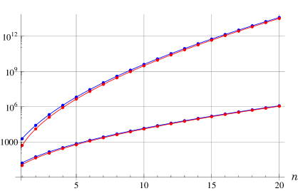
Figure 1. Absolute values of the Fourier coefficients of level-$2$. Blue dots and curves denote respectively exact and asymptotic values of $\Sigma_{(2,0,0)}^{(1)}$ and $\Sigma_{(1,1,0)}^{(1)}$. Red dots and curves are for $\Sigma_{(2,0,0)}^{(2)}$ and $\Sigma_{(1,1,0)}^{(2)}$.

We shall comment on a relationship between $Z_{X_{2}^{(1)}}$ and $Z_{X_{2}^{(2)}}$, and show that the Poincaré–Maass series (3.16) is merely a holomorphic Jacobi form when the polar parts are suitably chosen. The Riemann addition formulae for the Jacobi theta series (see, e.g., Ref. 35) read as

$$\left(\frac{\theta_{01}(z;\tau)}{\theta_{01}(0;\tau)}\right)^{2} =\left(\frac{\theta_{10}(z;\tau)}{\theta_{10}(0;\tau)}\right)^{2}+\frac{1}{4}\,\left(\frac{\theta_{00}(0;\tau)}{\eta(\tau)}\right)^{4}\,\left(\frac{\theta_{11}(z;\tau)}{\eta(\tau)}\right)^{2}$$ (4.16)

$$=\left(\frac{\theta_{00}(z;\tau)}{\theta_{00}(0;\tau)}\right)^{2}+\frac{1}{4}\,\left(\frac{\theta_{10}(0;\tau)}{\eta(\tau)}\right)^{4}\,\left(\frac{\theta_{11}(z;\tau)}{\eta(\tau)}\right)^{2},$$

which shows

$$Z_{X_{2}^{(1)}}(z;\tau)-24\,Z_{X_{2}^{(2)}}(z;\tau) = 3\,\frac{E_{4}(\tau)}{\left[\eta(\tau)\right]^{10}}\,\left[\Psi_{2}^{(2)}(\tau)\,B_{2}^{(1)}(z;\tau)-\Psi_{2}^{(1)}(\tau)\,B_{2}^{(2)}(z;\tau)\right]$$ (4.17)

$$= 3\,\left[\phi_{-2,1}(z;\tau)\right]^{2}\,E_{4}(\tau).$$

where $\Psi^{(a)}_{k}(\tau)$’s are defined in (2.14).

(4.17) shows that $\boldsymbol{\Phi}_{2}(\tau)$ defined by

$${\boldsymbol{\Phi}}_{2}(\tau) =\frac{E_{4}(\tau)}{\left[\eta(\tau)\right]^{10}}\,\begin{pmatrix}\Psi_{2}^{(2)}(\tau)\\[2.84526pt] -\Psi_{2}^{(1)}(\tau)\end{pmatrix}=\frac{E_{4}(\tau)}{\left[\eta(\tau)\right]^{10}}\,\begin{pmatrix}2\,\frac{\left[\eta(\tau)\,\eta(4\,\tau)\right]^{2}}{\eta(2\,\tau)}\\[2.84526pt] -\frac{\left[\eta(2\,\tau)\right]^{5}}{\left[\eta(4\,\tau)\right]^{2}}\end{pmatrix}$$ (4.18)

$$=\begin{pmatrix}q^{-\frac{1}{12}}\,\left[2+496\,q+8250\,q^{2}+70000\,q^{3}+434500\,q^{4}+2184512\,q^{5}+\cdots\right]\\[2.84526pt] q^{-\frac{1}{3}}\,\left[-1-250\,q-4620\,q^{2}-43000\,q^{3}-282632\,q^{4}-1484252\,q^{5}-\cdots\right]\end{pmatrix},$$

is a holomorphic vector-valued modular form which transforms as (3.9) with $k=2$. Existence of this form follows from the fact that one of two Jacobi forms with index-2, $\left[\phi_{-2,1}\right]^{2}\,E_{4}$, vanishes at $z=0$. In fact when we substitute $\left[\phi_{-2,1}\right]^{2}\,E_{4}$ for $\widehat{J}_{k}(z;\tau)$ in (3.4)

$$\boldsymbol{\Phi}_{2}(\tau)=-\mathrm{i}\,\left[\eta(\tau)\right]^{3}\,E_{4}(\tau)\,\int_{z_{0}}^{z_{0}+1}\frac{\theta_{11}(2\,z;\tau)}{\left[\theta_{11}(z;\tau)\right]^{2}}\,\left[\phi_{-2,1}(z;\tau)\right]^{2}\,\begin{pmatrix}q^{-\frac{1}{12}}\,\mathrm{e}^{-2\,\pi\,\mathrm{i}\,z}\\[2.84526pt] q^{-\frac{1}{3}}\,\mathrm{e}^{-4\,\pi\,\mathrm{i}\,z}\end{pmatrix}\,\mathrm{d}z,$$

the integrand is non-singular and is well-defined because of the zero of $\left[\phi_{-2,1}\right]^{2}$.

From (4.15), we obtain

$$\boldsymbol{\Phi}_{2}(\tau)=-{1\over 3}\,\begin{pmatrix}\Sigma_{(2,0,0)}^{(1)}(\tau)\\ \Sigma_{(2,0,0)}^{(2)}(\tau)\end{pmatrix}+8\,\begin{pmatrix}\Sigma_{(1,1,0)}^{(1)}(\tau)\\ \Sigma_{(1,1,0)}^{(2)}(\tau)\end{pmatrix}.$$

In these combinations $\Sigma$ functions acquire good modular transformation properties.

4.2.2. Level-$3$

We have three Jacobi forms with weight-$0$ and index-$3$. Each Jacobi form $Z_{X_{3}^{(a)}}$ is defined and decomposed as follows;

$$\begin{aligned} \frac{1}{4}\,Z_{X_{3}^{(1)}}(z;\tau)&=64\,\left[\left(\frac{\theta_{10}(z;\tau)}{\theta_{10}(0;\tau)}\right)^{6}+\text{others}\right]\\ &=142\operatorname{ch}_{3,\frac{3}{4},0}^{\widetilde{R}}(z;\tau)-14\,\operatorname{ch}_{3,\frac{3}{4},\frac{1}{2}}^{\widetilde{R}}(z;\tau)+6\,\operatorname{ch}_{3,\frac{3}{4},1}^{\widetilde{R}}(z;\tau)-\operatorname{ch}_{3,\frac{3}{4},\frac{3}{2}}^{\widetilde{R}}(z;\tau)\\ &\qquad+q^{-\frac{1}{16}}\,\left[5306\,q+145410\,q^{2}+2248049\,q^{3}+\cdots\right]\,B_{3}^{(1)}(z;\tau)\\ &\qquad+q^{-\frac{1}{4}}\,\left[-1856\,q-97368\,q^{2}-1848000\,q^{3}+\cdots\right]\,B_{3}^{(2)}(z;\tau)\\ &\qquad+q^{-\frac{9}{16}}\,\left[-21\,q+17927\,q^{2}+510797\,q^{3}+\cdots\right]\,B_{3}^{(3)}(z;\tau),\end{aligned}$$

$$\begin{aligned} Z_{X_{3}^{(2)}}(z;\tau)&=8\,\left[\left(\frac{\theta_{10}(z;\tau)}{\theta_{10}(0;\tau)}\right)^{4}\,\left(\frac{\theta_{00}(z;\tau)}{\theta_{00}(0;\tau)}\right)^{2}+\text{others}\right]\\ &=29\operatorname{ch}_{3,\frac{3}{4},0}^{\widetilde{R}}(z;\tau)-8\,\operatorname{ch}_{3,\frac{3}{4},\frac{1}{2}}^{\widetilde{R}}(z;\tau)+\operatorname{ch}_{3,\frac{3}{4},1}^{\widetilde{R}}(z;\tau)\\ &\qquad+q^{-\frac{1}{16}}\,\left[294\,q+2466\,q^{2}+14302\,q^{3}+\cdots\right]\,B_{3}^{(1)}(z;\tau)\\ &\qquad+q^{-\frac{1}{4}}\,\left[72\,q+261\,q^{2}+504\,q^{3}+\cdots\right]\,B_{3}^{(2)}(z;\tau)\\ &\qquad+q^{-\frac{9}{16}}\,\left[-18\,q-644\,q^{2}-5544\,q^{3}-\cdots\right]\,B_{3}^{(3)}(z;\tau),\end{aligned}$$

$$\begin{aligned} Z_{X_{3}^{(3)}}(z;\tau)&=4\,\left(\frac{\theta_{10}(z;\tau)}{\theta_{10}(0;\tau)}\right)^{2}\,\left(\frac{\theta_{00}(z;\tau)}{\theta_{00}(0;\tau)}\right)^{2}\,\left(\frac{\theta_{01}(z;\tau)}{\theta_{01}(0;\tau)}\right)^{2}\\ &=2\operatorname{ch}_{3,\frac{3}{4},0}^{\widetilde{R}}(z;\tau)-\operatorname{ch}_{3,\frac{3}{4},\frac{1}{2}}^{\widetilde{R}}(z;\tau)\\ &\qquad+q^{-\frac{1}{16}}\,\left[7\,q+21\,q^{2}+43\,q^{3}+94\,q^{4}+\cdots\right]\,B_{3}^{(1)}(z;\tau)\\ &\qquad+q^{-\frac{1}{4}}\,\left[8\,q+24\,q^{2}+56\,q^{3}+112\,q^{4}+\cdots\right]\,B_{3}^{(2)}(z;\tau)\\ &\qquad+q^{-\frac{9}{16}}\,\left[3\,q+14\,q^{2}+28\,q^{3}+69\,q^{4}+\cdots\right]\,B_{3}^{(3)}(z;\tau).\end{aligned}$$

Polar parts are given by

$$\hskip-42.67912pt\left.\begin{pmatrix}\Sigma_{(3,0,0)}^{(1)}(\tau)\\ \Sigma_{(3,0,0)}^{(2)}(\tau)\\ \Sigma_{(3,0,0)}^{(3)}(\tau)\end{pmatrix}\right|_{\text{polar}}\hskip-19.91692pt=\begin{pmatrix}116\,q^{-\frac{1}{16}}\\[2.84526pt] 32\,q^{-\frac{1}{4}}\\[2.84526pt] 4\,q^{-\frac{9}{16}}\end{pmatrix},\hskip 8.53581pt\left.\begin{pmatrix}\Sigma_{(2,1,0)}^{(1)}(\tau)\\ \Sigma_{(2,1,0)}^{(2)}(\tau)\\ \Sigma_{(2,1,0)}^{(3)}(\tau)\end{pmatrix}\right|_{\text{polar}}\hskip-19.91692pt=\begin{pmatrix}10\,q^{-\frac{1}{16}}\\[2.84526pt] q^{-\frac{1}{4}}\\[2.84526pt] 0\end{pmatrix},\hskip 8.53581pt\left.\begin{pmatrix}\Sigma_{(1,1,1)}^{(1)}(\tau)\\ \Sigma_{(1,1,1)}^{(2)}(\tau)\\ \Sigma_{(1,1,1)}^{(3)}(\tau)\end{pmatrix}\right|_{\text{polar}}\hskip-19.91692pt=\begin{pmatrix}q^{-\frac{1}{16}}\\[2.84526pt] 0\\[2.84526pt] 0\end{pmatrix}.$$

We have numerically checked that (3.19) with these polar parts reproduce above massive coefficients in $Z_{X_{3}^{(a)}}$. The theta function in (3.17) vanishes also in this case.

The bases of (2.27) are written as

$$\begin{pmatrix}\left[\phi_{0,1}\right]^{3}\\[2.84526pt] \left[\phi_{-2,1}\right]^{2}\,\phi_{0,1}\,E_{4}\\[2.84526pt] \left[\phi_{-2,1}\right]^{3}\,E_{6}\end{pmatrix}=\begin{pmatrix}1&24&96\\ 1&0&-48\\ 1&-12&96\end{pmatrix}\,\begin{pmatrix}\frac{1}{4}\,Z_{X_{3}^{(1)}}\\[2.84526pt] Z_{X_{3}^{(2)}}\\[2.84526pt] Z_{X_{3}^{(3)}}\end{pmatrix}.$$ (4.20)

We note that the elliptic genus for the Calabi–Yau manifold was studied in Ref. 21 where used is

$$Z_{X_{3}^{(3)}}(z;\tau)=\frac{1}{4}\,\phi_{0,3}(z;\tau).$$

We denote $X_{3}(n_{2},n_{3})$ as the complex 6-dimensional hyperKähler manifold whose elliptic genus for $X_{3}(n_{2},n_{3})$ is given by (4.1) with $d_{3}=3$. We have

$$\begin{gathered}Z_{X_{3}(n_{2},n_{3})}(0;\tau)=768+48\,n_{2}+4\,n_{3},\\[5.69054pt] Z_{X_{3}(n_{2},n_{3})}\left(\frac{1}{2};\tau\right)=\left(512+16\,n_{2}\right)+\cdots,\\[5.69054pt] Z_{X_{3}(n_{2},n_{3})}\left(\frac{1+\tau}{2};\tau\right)=-4\,q^{-\frac{3}{2}}+\cdots.\end{gathered}$$ (4.21)

Referring to the generating function (4.3), we see $K3^{[3]}=X_{3}(40,128)$, and we recover the topological invariants as

$$\chi_{K3^{[3]}} =3200, \sigma_{K3^{[3]}} =1152, \widehat{A}_{K3^{[3]}} =4.$$ (4.22)

We note that the character decomposition is given by

$$Z_{K3^{[3]}}(z;\tau) =1984\,\operatorname{ch}_{3,\frac{3}{4},0}^{\widetilde{R}}(z;\tau)-504\,\operatorname{ch}_{3,\frac{3}{4},\frac{1}{2}}^{\widetilde{R}}(z;\tau)+64\,\operatorname{ch}_{3,\frac{3}{4},1}^{\widetilde{R}}(z;\tau)-4\,\operatorname{ch}_{3,\frac{3}{4},\frac{3}{2}}^{\widetilde{R}}(z;\tau)$$

$$\qquad+q^{-\frac{1}{16}}\,\left[33880\,q+682968\,q^{2}+9569780\,q^{3}+\cdots\right]\,B_{3}^{(1)}(z;\tau)$$

$$\qquad+q^{-\frac{1}{4}}\,\left[-3520\,q-375960\,q^{2}-7364672\,q^{3}+\cdots\right]\,B_{3}^{(2)}(z;\tau)$$

$$\qquad+q^{-\frac{9}{16}}\,\left[-420\,q+47740\,q^{2}+1825012\,q^{3}+\cdots\right]\,B_{3}^{(3)}(z;\tau).$$

5. Conclusion and Discussion

In this paper we have studied the general properties of the elliptic genera of arbitrary hyperKähler manifolds of complex dimension $2k$.

Using the Rademacher expansion we have shown that the multiplicities of the (overall) half-BPS states increase like an exponential and behaves like

$$\exp\left(2\,\pi\,\sqrt{k\,n}\right)$$ (5.1)

for large values of $k$. We would like to identify this phenomenon as the entropy carried by the hyperKähler manifolds.

In the standard model of D1-D5 black holes of string theory compactified on $K3\times S^{1}$ with $Q_{5}$ D5 and $Q_{1}$ D1 branes, the effective theory is a 2-dimensional non-linear $\sigma$-model with the target space being the symmetric product of $k=Q_{1}\,Q_{5}$ $K3$ surfaces. Entropy of the black hole is given by [42]

$$S_{BH}=2\,\pi\,\sqrt{Q_{1}\,Q_{5}\,n},$$ (5.2)

where $n$ is the momentum around $S^{1}$. We note that (5.1) and (5.2) agree with each other.

Our proposal of the intrinsic entropy for hyperKähler manifolds must be strengthened by examining similar phenomena in other types of manifolds: we expect that a manifold with a reduced holonomy in general possesses an intrinsic entropy. In the case of Calabi-Yau manifolds one uses the $\mathcal{N}$=2 SCA and the analysis is more or less similar to the case of hyperKähler manifolds. We plan to report on the results of Calabi-Yau manifolds in a subsequent publication  [12]. On the other hand, in the case of $G_{2}$ and spin(7) manifolds the relevant algebraic structures are not yet known. It is a challenging problem to develop the representation theory and analyze the elliptic genera for these manifolds.

Appendix A Harmonic Maass Form

The functions $f(\tau)$ is called the harmonic Maass form with weight $k\in\frac{1}{2}\mathbb{Z}$ on $\Gamma\in\left\{\Gamma_{1}(N),\Gamma_{0}(N)\right\}$ if the followings are fulfilled [5, 37];

• for $\gamma=\left(\begin{smallmatrix}a&b\\ c&d\end{smallmatrix}\right)\in\Gamma$, we have

  $$f\left(\gamma(\tau)\right)=\begin{cases}(c\,\tau+d)^{k}\,f(\tau),&\text{for $k\in\mathbb{Z}$},\\[5.69054pt] \displaystyle\left(\frac{c}{d}\right)^{2k}\,\epsilon_{d}^{~{}-2k}\,(c\,\tau+d)^{k}\,f(\tau),&\text{for $k\in\mathbb{Z}+\frac{1}{2}$},\end{cases}$$ (A.1)

  where $\left(\frac{c}{d}\right)$ is the Legendre symbol, and $\epsilon_{d}$ is defined by

  $$\epsilon_{d}=\begin{cases}1&\text{for $d=1\mod 4$},\\ \mathrm{i}&\text{for $d=3\mod 4$},\end{cases}$$

• $f(\tau)$ is an eigenfunction of the hyperbolic Laplacian (2.25),

  $$\Delta_{k}f(\tau)=0,$$ (A.2)

• there exists a polynomial such that

  $$f(\tau)-\sum_{n\leq 0}c(n)\,q^{n}=\mathcal{O}\left(\mathrm{e}^{-\epsilon v}\right),$$ (A.3)

  for $v=\Im\tau\to\infty$ and some $\epsilon>0$.

References

• [1] G. E. Andrews, Mock theta functions, in L. Ehrenpreis and R. C. Gunning, eds., Theta Functions — Bowdoin 1987, Proc. Symp. Pure Math. 49 (part 2), pp. 283–298, Amer. Math. Soc., Providence, 1989.
• [2] K. Bringmann and K. Ono, The $f(q)$ mock theta function conjecture and partition ranks, Invent. Math. 165, 243–266 (2006).
• [3] ———, Coefficients of harmonic Maass forms, Proceedings of the 2008 University of Florida Conference on Partitions, $q$-Series, and Modular Forms, to appear.
• [4] J. H. Bruinier, Borcherds Products on $O(2,\ell)$ and Chern Classes of Heegner Divisors, Lecture Notes in Mathematics 1780, Springer, Berlin, 2002.
• [5] J. H. Bruinier and J. Funke, On two geometric theta lifts, Duke Math. J. 125, 45–90 (2004).
• [6] M. Cvetič and F. Larsen, Near horizon geometry of rotating black holes in five dimensions, Nucl. Phys. B 531, 239–255 (1998) [hep-th/9805097].
• [7] R. Dijkgraaf, J. Maldacena, G. Moore, and E. Verlinde, A black hole Farey tail [hep-th/0005003].
• [8] R. Dijkgraaf, G. Moore, E. Verlinde, and H. Verlinde, Elliptic genera of symmetric products and second quantized strings, Commun. Math. Phys. 185, 197–209 (1997) [hep-th/9608096].
• [9] F. J. Dyson, A walk through Ramanujan’s garden, in Ramanujan Revisited, pp. 7–28, Academic Press, Boston, 1988.
• [10] T. Eguchi and K. Hikami, Superconformal algebras and mock theta functions, J. Phys. A: Math. Theor. 42, 304010 (2009), 23 pages [arXiv:0812.1151].
• [11] ———, Superconformal algebras and mock theta functions 2. Rademacher expansion for K3 surface, Commun. Number Theory Phys. 3, 531–554 (2009) [arXiv:0904.0911].
• [12] ———, in preparation.
• [13] T. Eguchi, H. Ooguri, A. Taormina, and S.-K. Yang, Superconformal algebras and string compactification on manifolds with SU($n$) holonomy, Nucl. Phys. B 315, 193–221 (1989).
• [14] T. Eguchi, Y. Sugawara, and A. Taormina, Liouville field, modular forms and elliptic genera, JHEP 2007, 119 (2007), 21 pages [hep-th/0611338].
• [15] ———, Modular forms and elliptic genera for ALE spaces [arXiv:0803.0377].
• [16] T. Eguchi and A. Taormina, Unitary representations of the $N=4$ superconformal algebra, Phys. Lett. B 196, 75–81 (1986).
• [17] ———, Character formulas for the $N=4$ superconformal algebra, Phys. Lett. B 200, 315–322 (1988).
• [18] ———, On the unitary representations of $N=2$ and $N=4$ superconformal algebras, Phys. Lett. B 210, 125–132 (1988).
• [19] M. Eichler and D. Zagier, The Theory of Jacobi Forms, Progress in Mathematics 55, Birkhäuser, Boston, 1985.
• [20] L. Göttsche, The Betti numbers of the Hilbert schemes of points on a smooth projective surface, Math. Ann. 286, 193–207 (1990).
• [21] V. Gritsenko, Elliptic genus of Calabi–Yau manifolds and Jacobi and Siegel modular forms, Algebra i Analiz 11, 100–125 (1999) [math/9906190].
• [22] D. A. Hejhal, The Selberg Trace Formula for PSL($2,\mathbb{R}$) Vol. 2, Lecture Notes in Mathematics 1001, Springer, Berlin, 1983.
• [23] K. Hikami, Mock (false) theta functions as quantum invariants, Regular & Chaotic Dyn. 10, 509–530 (2005) [math-ph/0506073].
• [24] ———, On the quantum invariant for the Brieskorn homology spheres, Int. J. Math. 16, 661–685 (2005) [math-ph/0405028].
• [25] ———, On the quantum invariant for the spherical Seifert manifold, Commun. Math. Phys. 268, 285–319 (2006) [math-ph/0504082].
• [26] ———, Hecke type formula for unified Witten–Reshetikhin–Turaev invariant as higher order mock theta functions, Int. Math. Res. Not. IMRN 2007, rnm022–32 (2007).
• [27] K. Hikami and A. N. Kirillov, Torus knot and minimal model, Phys. Lett. B 575, 343–348 (2003) [hep-th/0308152].
• [28] N. Hitchin and J. Sawon, Curvature and characteristic numbers of hyper-Kähler manifolds, Duke Math. J. 106, 599–615 (2001) [math/9908114].
• [29] L. C. Jeffrey, Chern–Simons–Witten invariants of lens spaces and torus bundles, and the semiclassical approximation, Commun. Math. Phys. 147, 563–604 (1992).
• [30] T. Kawai, Y. Yamada, and S.-K. Yang, Elliptic genera and $N=2$ superconformal field theory, Nucl. Phys. B 414, 191–212 (1994) [hep-th/9306096].
• [31] R. Lawrence and D. Zagier, Modular forms and quantum invariants of 3-manifolds, Asian J. Math. 3, 93–107 (1999).
• [32] A. Maloney and E. Witten, Quantum gravity partition function in three dimensions [arXiv:0712:0155].
• [33] J. Manschot and G. W. Moore, A modern Farey tail [arXiv:0712.0573].
• [34] G. Moore, Strings and arithmetic, in P. Cartier, B. Julia, and P. Moussa, eds., Frontiers in Number Theory, Physics and Geometry II, pp. 303–359, Springer, Berlin, 2006 [hep-th/0401049].
• [35] D. Mumford, Tata Lectures on Theta I, Progress in Mathematics 28, Birkhäuser, Boston, 1983.
• [36] K. Ono, The Web of Modularity: Arithmetic of the Coefficients of Modular Forms and $q$-Series, CMBS Regional Conference Series in Mathematics 102, Amer. Math. Soc., Providence, 2004.
• [37] ———, Unearthing the visions of a master: harmonic Maass forms and number theory, Current Developments in Mathematics 2008, 347–454 (2009).
• [38] H. Rademacher, Topics in Analytic Number Theory, Grund. Math. Wiss. 169, Springer, New York, 1973.
• [39] N. Yu. Reshetikhin and V. G. Turaev, Invariants of 3-manifolds via link polynomials and quantum groups, Invent. Math. 103, 547–597 (1991).
• [40] J.-P. Serre and H. Stark, Modular Forms of weight $1/2$, in J.-P. Serre and D. Zagier, eds., Modular Functions of One Variable VI, Lecture Notes in Mathematics 627, pp. 27–67, 1977.
• [41] N. Skoruppa and D. Zagier, A trace formula for Jacobi forms, J. Reine Angew. Math. 393, 168–198 (1989).
• [42] A. Strominger and C. Vafa, Microscopic origin of the Bekenstein–Hawking entropy, Phys. Lett. B 379, 99–104 (1996) [hep-th/9601029].
• [43] E. T. Whittaker and G. N. Watson, A Course of Modern Analysis, Cambridge Univ. Press, Cambridge, 1927, 4th ed.
• [44] E. Witten, Elliptic genera and quantum field theory, Commun. Math. Phys. 109, 525–536 (1987).
• [45] ———, Quantum field theory and the Jones polynomial, Commun. Math. Phys. 121, 351–399 (1989).
• [46] D. Zagier, Vassiliev invariants and a strange identity related to the Dedekind eta-function, Topology 40, 945–960 (2001).
• [47] ———, Ramanujan’s mock theta functions and their applications [d’après Zwegers and Bringmann–Ono], Séminaire Bourbaki 986 (2006–2007).
• [48] S. P. Zwegers, Mock Theta Functions, Ph.D. thesis, Universiteit Utrecht (2002) [arXiv:0807.4834].