Molecular and Atomic Gas in the Large Magellanic Cloud II. Three-dimensional Correlation between CO and HI

Abstract

We compare the CO ($J=$1–0) and HI emission in the Large Magellanic Cloud (LMC) in three dimensions, i.e. including a velocity axis in addition to the two spatial axes, with the aim of elucidating the physical connection between giant molecular clouds (GMCs) and their surrounding HI gas. The CO $J=$1–0 dataset is from the second NANTEN CO survey and the HI dataset is from the merged Australia Telescope Compact Array (ATCA) and Parkes Telescope surveys. The major findings of our analysis are: 1) GMCs are associated with an envelope of HI emission, 2) in GMCs [average CO intensity] $\propto$ [average HI intensity]^1.1±0.1 and 3) the HI intensity tends to increase with the star formation activity within GMCs, from Type I to Type III. An analysis of the HI envelopes associated with GMCs shows that their average linewidth is 14 km s^-1 and the mean density in the envelope is 10 cm^-3. We argue that the HI envelopes are gravitationally bound by GMCs. These findings are consistent with a continual increase in the mass of GMCs via HI accretion at an accretion rate of 0.05 $M_{\sun}$yr^-1 over a time scale of 10 Myr. The growth of GMCs is terminated via dissipative ionization and/or stellar-wind disruption in the final stage of GMC evolution.

1 Introduction

Giant molecular clouds (GMCs), the most massive aggregations of interstellar matter with $10^{5-6}M_{\sun}$, are the principal sites of star formation in galaxies. It is important to understand how GMCs are formed out of the less dense atomic interstellar gas in order to understand galactic evolution. The interstellar HI gas has densities of less than several 10 cm^-3 while molecular clouds have densities larger than 100 cm^-3. It is reasonable to assume that HI is being converted into H₂ either by thermal/gravitational instabilities and/or shock compressions, although the detailed processes of this conversion are not yet well-understood. Sato & Fukui (1978) and Hasegawa, Sato, & Fukui (1983) identified cold HI gas associated with GMCs in M17 and W3/4 and suggested that the cold HI gas may be converted into molecular gas for these GMCs. Subsequently, Wannier et al (1983) showed that five molecular clouds are associated with warm HI envelopes and suggested that such HI envelopes may be common around GMCs. Nonetheless, associations between GMCs and HI envelopes are difficult to identify systematically throughout the Galactic disk, since GMCs samples are restricted to the solar vicinity due to the crowding effects (Andersson, Wannier, & Morris 1991). As a consequence, the GMC-HI association has not been well established.

The Magellanic system – including the LMC, the SMC and the Bridge – is an ideal laboratory to study star formation and molecular cloud evolution because of its proximity to the Milky Way (e.g., Fukui et al 1999; Mizuno et al. 2001; Mizuno et al. 2006; Fukui et al. 2008; Ott et al. 2008; Kawamura et al, 2009). We expect that the Magellanic system can also shed light on the physical connection between GMCs and their atomic surroundings. Indeed, the LMC may offer the best place for such a study because of its nearly face-on orientation and level of star formation activity. The LMC’s molecular cloud population, which is best traced via the CO emission, provides a key to understand the galaxy’s star formation. Molecular clouds are able to highlight the location of star formation due to their highly clumped distribution in both space and velocity. The LMC’s atomic gas, by contrast, has lower densities and is only weakly coupled to sites of active star formation, but it is the most promising candidate for the mass reservoir of GMC formation (e.g., Blitz et al. 2007). We note, moreover, that cold HI gas has been detected in the LMC (e.g., Dickey et al. 1994), and that the correlation between CO and HI may provide crucial observational evidence about the molecular cloud formation process.

Wong et al. (2009) compared the HI and CO emission throughout the LMC on a pixel-by-pixel basis using the second NANTEN CO and ATCA+Parkes HI datasets. These authors studied correlations between the integrated CO and HI intensities, where the latter was integrated over all velocities with HI emission or over individual Gaussian components. They found that CO emission is associated with high intensity HI gas but that intense HI emission is not always associated with CO. They also discovered a weak tendency for CO to be associated with HI components that have relatively low velocity dispersion. This suggests that energy dissipation of the HI gas may be required for the formation of molecular clouds. Following the global analysis by Wong et al. (2009), we focus here on the HI associated with individual GMCs in the LMC. In order to address this issue, we conduct a detailed comparison between the CO and HI emission in three dimensions, i.e. $(x,y,v)$, at a spatial resolution of $\sim$40 pc and a velocity resolution of 1.7 km ss^-1. The present study is complementary to the work by Wong et al. (2009); in conjunction, the two studies provide a new insight into the CO-HI connection. In section 2, we briefly review the basic observational properties of GMCs in the LMC. In section 3, we describe our method of analysing the CO-HI correlation and present our results. We discuss the physical interpretation of our results in section 4 and provide a summary of our major conclusions in section 5.

2 GMCs in the LMC; the second NANTEN CO survey

The LMC is extended by more than 30 square degrees across the sky and it has been a difficult task to make a systematic survey of the CO emission at angular resolutions sufficient to resolve individual GMCs. Fukui et al. (1999) made such a survey in the 2.6mm CO line with the NANTEN 4m mm-wave telescope and published the first results in Fukui et al. (1999). Subsequently, these authors completed another survey of the LMC, improving the sensitivity by a factor of two. The second NANTEN CO survey has cataloged 272 GMCs (Fukui et al. 2008). The basic physical parameters of GMCs in the LMC are similar to those in the Milky Way and other nearby galaxies. Their masses range from $\sim 10^{5}M_{\sun}$ to $\sim 10^{6}M_{\sun}$; the mass spectrum is quite steep with a slope of $dN/dM\sim M^{-2}$. The X factor, the ratio of the H₂ column density to CO intensity, is $\sim 7\times 10^{20}$ cm^-2 (K km s^-1) ^-1 (Fukui et al. 2008; Blitz et al. 2007). The complete sampling of the NANTEN survey has also allowed us to make a statistical study of GMCs with various young objects including HII regions and young stellar clusters. Kawamura et al. (2009) confirmed that there are three classes of GMCs, that can be categorised according to their association with young star clusters as originally indicated in the analysis of the first NANTEN LMC survey (Fukui et al. 1999; Yamaguchi et al. 2001). Type I GMCs show no signs of active star formation in the sense that no O stars are being formed. Type II GMCs are associated with small HII region(s), indicating the formation of isolated O stars, but do not host any stellar clusters identified by Bica et al. (1996). Type III GMCs are actively forming stars as shown by their association with large HII regions and young stellar clusters. These classes are interpreted as an evolutionary sequence from Type I to III; the lifetime of a GMC is estimated to be a few $\times$ 10 Myr in total (Kawamura et al. 2009). The stage after Type III is likely to be a very violent dissipation of the GMC due to the UV photons and stellar winds produced by the nascent clusters, as seen spectacularly in the region of 30 Dor (Yamaguchi et al. 2001). A comparison of the physical parameters of the GMCs shows that the size and mass of the clouds tend to increase from Type I/II to Type III. A summary of the average mass and size for the three GMC classes is presented in Table 1, as taken from Kawamura et al. (2009).

3 Correlation between CO and HI

3.1 3-D correlation

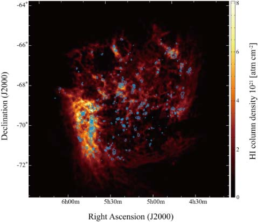
Figure 1: HI integrated intensity image (Kim et al. 2003) with contours of the CO integrated intensity (Fukui et al. 2008). The contour levels begin at 1.2 K km s^-1 and have 3.6 K km s^-1 intervals.

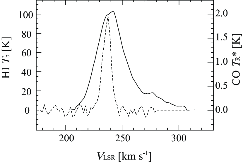
Figure 2: An example of the HI and CO line profiles at $\alpha$(J2000) $=$ 5^h39^m38^s, and $\delta$(J2000) $=-69\arcdeg 44\arcmin 46\arcsec$.

Previous studies of star formation in galaxies have employed 2-dimensional (2-D) maps of HI intensity with large spatial averaging on scales between $\sim$100 pc and 1 kpc (e.g., Schmidt 1972; Kennicut et al. 1988). Here, we make a 3-D comparison between the CO and HI in the LMC where the 3-D datacubes have a velocity axis in addition to two spatial axes projected on the sky. Preliminary results of the comparison have been published elsewhere (Fukui 2007). We use the 3-D datacube of CO obtained with NANTEN (Fukui et al. 2008) and an HI datacube obtained with ATCA and Parkes (Kim et al. 2003). The CO emission traces GMCs and the HI emission traces less dense atomic gas. Figure 1 shows an overlay of the velocity-integrated intensities of the CO and HI emission; from this, it is clear that GMCs in the LMC tend to be located towards HI filaments or local HI peaks, suggesting that HI is a prerequisite for GMC formation (Blitz et al. 2007). However, it is also clear that there are many HI peaks and filaments without CO emission (Wong et al. 2009). Figure 2 shows typical CO and HI line profiles in the LMC. The CO emission is highly localized in velocity: the HI emission ranges over 100 km s^-1 while the CO emission has a typical linewidth of less than 10 km s^-1. We note that the large velocity dispersion of HI may be dominated by physically unrelated velocity components along the line of sight, i.e. the HI gas associated with the GMC may only be the small fraction of HI with velocities close to that of the CO emission. Previous studies of the CO-HI connection that use velocity integrated 2-D maps may therefore overestimate the intensity of the associated HI emission along each line of sight. By making use of the velocity dimension, the present 3-D analysis may allow us to identify the HI gas that is physically connected to the GMCs. The NANTEN and ATCA+Parkes datacubes have somewhat different spatial and velocity resolutions, so we have convolved both datasets to a spatial resolution of 40 pc $\times$ 40 pc, and a velocity resolution of 1.7 km s^-1. The total number of 3-D pixels is approximately $2\times 10^{6}$ across the area of surveyed by NANTEN. The HI and CO intensities are expressed in units of $T_{\rm b}$(K) and $T^{*}_{\rm R}$ (K); the $3\sigma$ noise levels of the HI and CO datacubes are 7.2 K and 0.21 K respectively. Strictly speaking, the one-to-one correspondence between a velocity and a position is not guaranteed because there is a chance that physically unrelated HI gas may have the same velocity as HI gas related to the GMC along the same line of sight. Our results identify the HI associated with GMCs and suggest that such contamination along individual sightlines may not be a serious problem. We further note that HI absorption towards background radio continuum sources does not affect significantly the HI intensity at the present spatial resolution, as verified toward 30 Dor, one of the brightest radio continuum sources in the LMC.

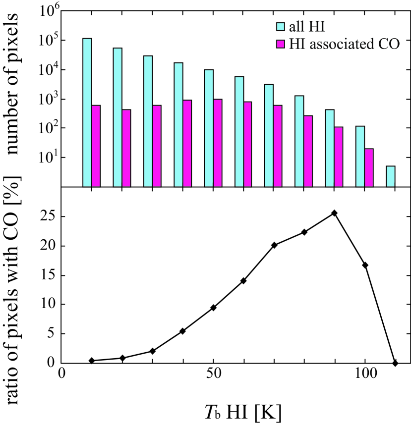
Figure 3: The HI and CO datacubes that use for our analysis have somewhat different spatial and velocity resolutions; we have convolved both datasets to a spatial resolution of 40 pc $\times$ 40 pc, and a velocity resolution of $\times$ 1.7 km s^-1 across the whole LMC. The pixels used in our analysis occupy the same volumes for both the HI and CO datasets. The $3\sigma$ detection limits for the CO and HI brightness are 0.21 K and 7.2 K respectively. (a) Histogram of the HI brightness temperature averaged within each 3-D pixel is shown in blue; the HI pixels with significant CO emission (i.e. $>3\sigma$) are marked in red. The width of the histogram bins is 10 K. (b) Ratio of the number of pixels with significant HI emission to those with significant CO emission within each 10 K bin.

Figure 3 shows a histogram of the HI intensity in the 3-D datacube. Pixels with the significant CO emission ($T^{*}_{\rm R}>$ 0.21 K) are shown in red. Throughout this paper, histograms always use the values of 3-D pixels with no spatial integration unless otherwise stated. The histogram in Figure 3 shows that the fraction of CO-detected pixels increases monotonically with the HI intensity, suggesting the HI intensity is a necessary condition to form GMCs, consistent with the conclusion by Wong et al. (2009). About one third of the pixels with $T_{\rm b}$(HI) of $\sim$ 90 K exhibit CO emission, but it seems that there is no sharp threshold value of HI intensity that is required for GMC formation.

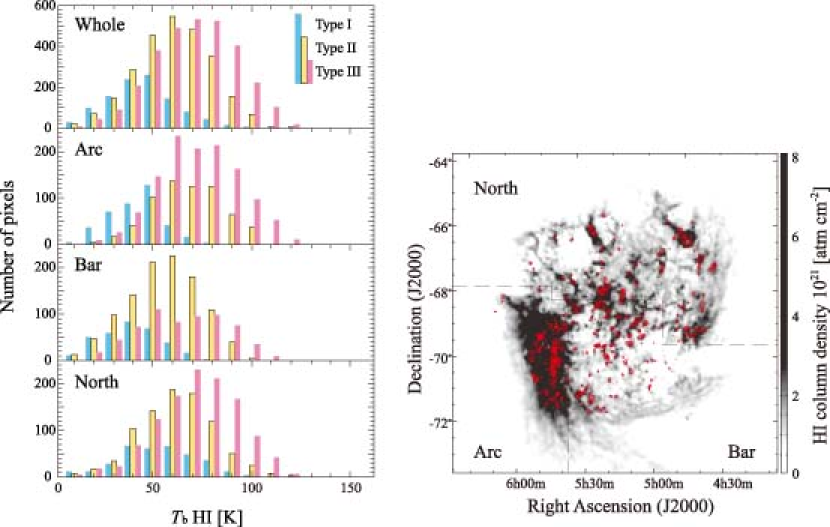
Figure 4: Histograms of the pixel-averaged HI brightness temperature where significant CO emission is detected for Type I (blue), Type II (yellow) and Type III (red) GMCs. Histograms are shown for the whole LMC, and for three different regions – Bar, North, and Arc – which are indicated in the right panel.

Figure 4 shows a histogram of the HI intensity for the three GMC types. Each pixel detected in CO belongs to one of the GMCs cataloged in Fukui et al (2008). Figure 4 clearly shows that the HI intensity tends to increase from Type I to Type III, although the dispersion is considerable. The average HI intensity for Types I, II and III GMCs across the LMC is $34\pm 16$ K($1\sigma$), $47\pm 17$ K and $56\pm 19$ K, i.e. the average HI intensity increases with the level of star formation activity within the GMC. In order to test for variation within the galaxy, we tentatively divide the galaxy into three regions, i.e., Bar, North and Arc, as shown in Figure 4(right). Histograms for each region, shown in the lower three panels of Figure 4, reveal the same trend, suggesting that the present trend is common over the whole LMC. The total number of the pixels in each region is 429,510, 666,060, and 405,093. Type I, Type II and Type III GMCs include 330, 1,065, and 639 pixels in the Bar region; 346, 878, and 1,158 pixels in the North region; and 389, 650, and 1,231 pixels in the Arc region.

Figure 5 shows the velocity channel maps of the HI distribution associated with Type I, Type II, and Type III GMCs. These channel maps clearly show that the HI is associated with the CO. The CO distribution has small structures of $\sim$ 100 pc or less and the HI appears to be associated with the GMC on larger scales of $\sim$ 100 to 400 pc. The HI emission is not always symmetric with respect to a GMC, even though HI typically envelopes each GMC. The associated HI is often elongated along the GMCs and the region of intense HI emission is usually $<$ 100 pc wide. The CO emission typically extends over a velocity range of $\sim 5$ km s^-1; beyond a few times this velocity range, the associated HI emission generally becomes much weaker or disappears.

3.2 Physical properties of the HI envelope

In general, it is a complicated task to derive reliable physical properties of the HI gas associated with a GMC because the HI profiles are a blend of several different components along the line of sight, making it difficult to select the HI gas that is physically connected to a GMC. Another obstacle is that the HI emission is spatially more extended than the CO emission and has a less clear boundary than the CO.

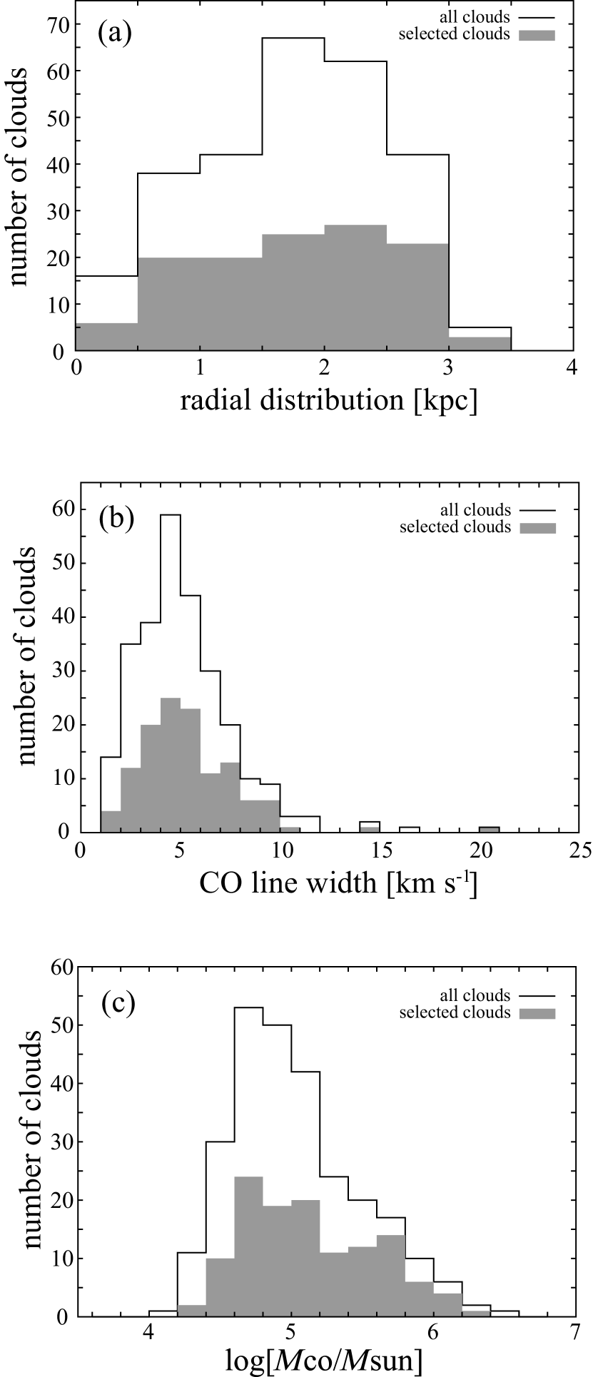
Figure 6: Histograms of three parameters, (a) the distance from the kinematic center of the galaxy (kpc), (b) the CO linwidth (kim s^-1) and (c) the CO cloud mass ($M_{\sun}$) for the 123 GMCs used in our analysis. The solid lines show the distribution of these properties for all the clouds in the Fukui et al. (2008) catalog; the gray shaded regions represent the distribution for the 123 selected GMCs (see also Table 2).

For our analysis, we first selected GMCs with simple single-peaked HI profiles from the Fukui et al (2008) catalog. The resulting sample consists of 123 GMCs in total. Their catalog numbers and basic physical properties, taken from Fukui et al. (2008), are listed in Table 2. For these GMCs, we tested whether there was a bias in their location with respect to the kinematic center of the galaxy, in their CO linewidth or in their molecular mass. The histograms in Figure 6 indicate that there is no particular trend for these properties of the selected GMCs compared to GMCs in the complete catalog, suggesting that there is no appreciable selection bias. We applied a Kolmogorov-Smirnov test to the three histograms and calculated maximum deviations of 0.031, 0.061 and 0.117 respectively for the three parameters. These values are less than the critical deviation, 0.129, for a conventional significance level of 0.05, confirming that there is no selection bias.

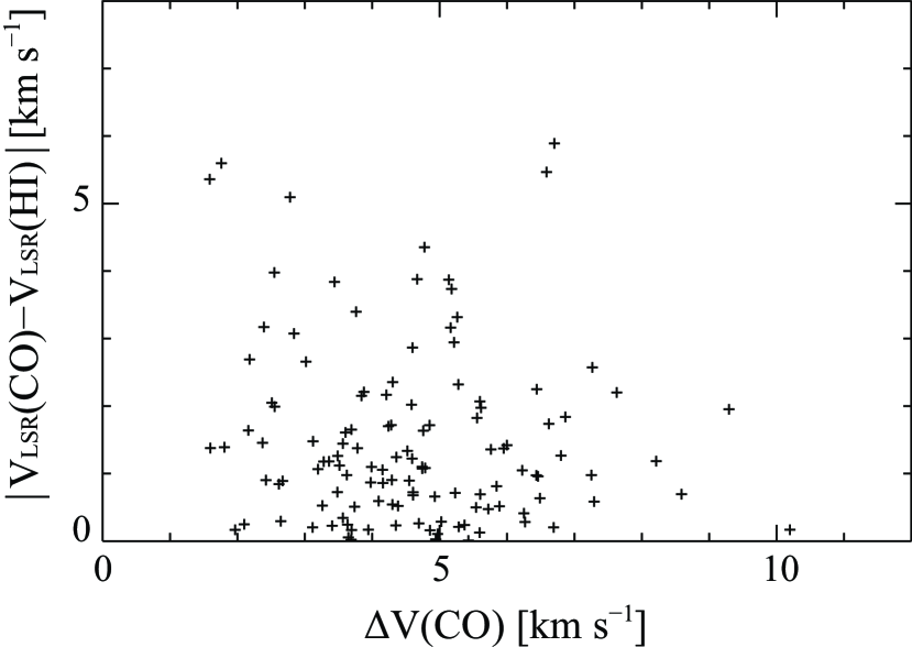
Figure 7: The absolute difference between the central velocity of the HI and CO emission, $|V_{\rm LSR}{\rm(CO)}-V_{\rm LSR}{\rm(HI)}|$, versus the CO linewidth, $\Delta V$ (CO) for the 123 GMCs in our sample. The dotted line shows $|V_{\rm LSR}{\rm(CO)}-V_{\rm LSR}{\rm(HI)}|=\Delta V$(CO).

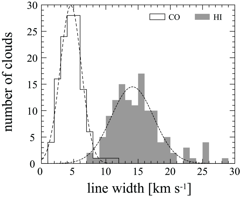
Figure 8: Histogram of the CO and HI linewidths toward the position of the CO peak position for the 123 selected GMCs. The dotted lines show Gaussian fits to the histograms. The mean values (standard derivations) for the CO and HI distributions are 4.6 (1.6) and 14.1 (3.3) km s^-1 respectively.

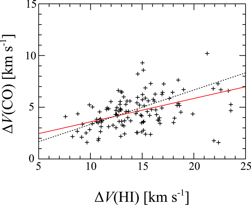
Figure 9: Plot of the CO versus HI linewidth for the 123 GMCs in our sample. The red line is the regression line $\Delta V{\rm(CO)}={\rm(}1.32\pm 0.04{\rm)}+{\rm(}0.23\pm 0.003{\rm)}\Delta V{\rm(HI)}$, and the dotted line shows $\Delta V{\rm(HI)}=3\times\Delta V{\rm(CO)}$. The Spearman rank correlation coefficient is 0.39.

Next, we made Gaussian fits to the HI and CO profiles towards the CO peak of each GMC. This procedure yields a peak intensity, peak velocity and half-power linewidth for each line profile (a summary is given for each GMC type in Table 1). Figure 7 shows the relation between the CO linewidth and the difference between the CO and HI peak velocities. We find the HI and CO peak velocities to be in good agreement, showing only a small scatter of less than a few km s^-1. Figure 8 shows two histograms of the HI and CO linewidths. We see that the HI linewidth is typically 14 km s^-1, roughly three times larger than that of CO. Figure 9 shows a correlation between HI and CO linewidths. The two quantities show a positive correlation with a correlation coefficient of 0.39. The correlation coefficient is determined using the Spearman rank method throughout the present paper. The kinematic properties of HI and CO, as illustrated in Figures 7 and 9, lend further support to a physical association between the HI and CO.

In order to estimate the size of the HI envelope surrounding each GMC, we construct an HI integrated intensity map of each GMC. First, we find the local peak in the HI intensity cube surrounding the CO emission, and then integrate the HI intensity over the velocity channels corresponding to the FWHM of the HI line profile at this peak position. Next we estimate the area, $S$, where the HI integrated intensity is greater than 80 % of the value at the local HI peak. We then calculate the radius of the HI envelope, $R$(HI) from its projected area, $S=\pi R({\rm HI})^{2}$. The HI integrated intensity is calculated for all the pixels with detectable CO emission; the spatial distribution of the HI emission generally shows a peak and a reasonably defined boundary. The 80 % level was chosen after a few trials using different levels; it is the maximum value for which a reasonable HI size is obtained for 116 of the 123 envelopes. While 80 % seems to be rather high for such a definition of a cloud envelope, the HI size can be unrealistically large compared to the CO cloud size along a filamentary HI distribution if we use a lower level such as 60 %; an example is shown in Figure 5b. The HI radius is then corrected for beam dilution by adopting Gaussian de-convolution with an HI FWHM of 2.6 arcmin, i.e. the same procedure that is applied to the radius of the GMC determined from the CO emission, $R$(CO) (Kawamura et al 2009). $R$(CO), the CO peak position, $R$(HI), the HI peak position, and the deviation between the peaks in parsecs, $\sqrt{(\Delta\alpha^{2}+\Delta\delta^{2})}$, are listed in Table 2. Seven clouds, for which $R$(HI) comprises only a few pixels, are denoted by asterisks. The physical extent of the HI envelopes can be as large as a few 100 pc. Ws long as we use the local HI peak of individual GMCs as our reference point, it seems difficult to contrive an alternative uniform definition of the envelope size is difficult using the present HI dataset.

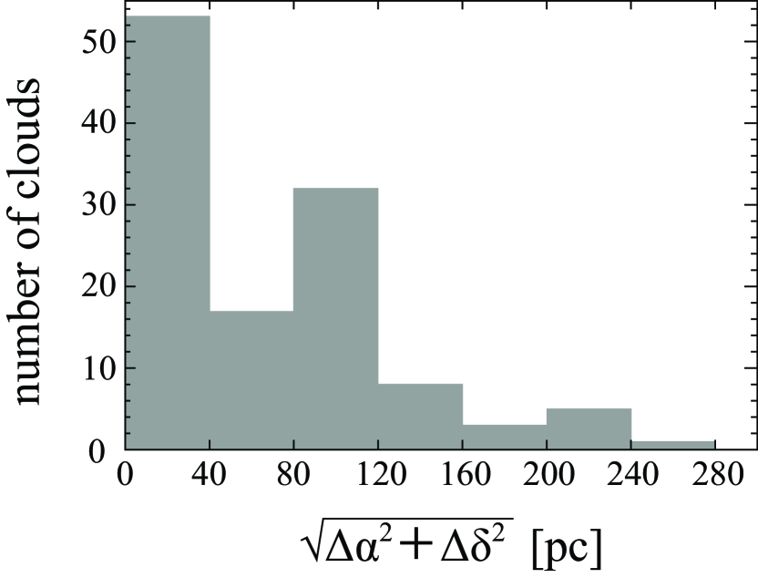
Figure 10: Histogram of the projected separation between the CO and HI peak positions, as listed Table 2. The separation between the CO and HI peak positions for four of the 123 clouds is greater than 300 pc; these clouds are not shown.

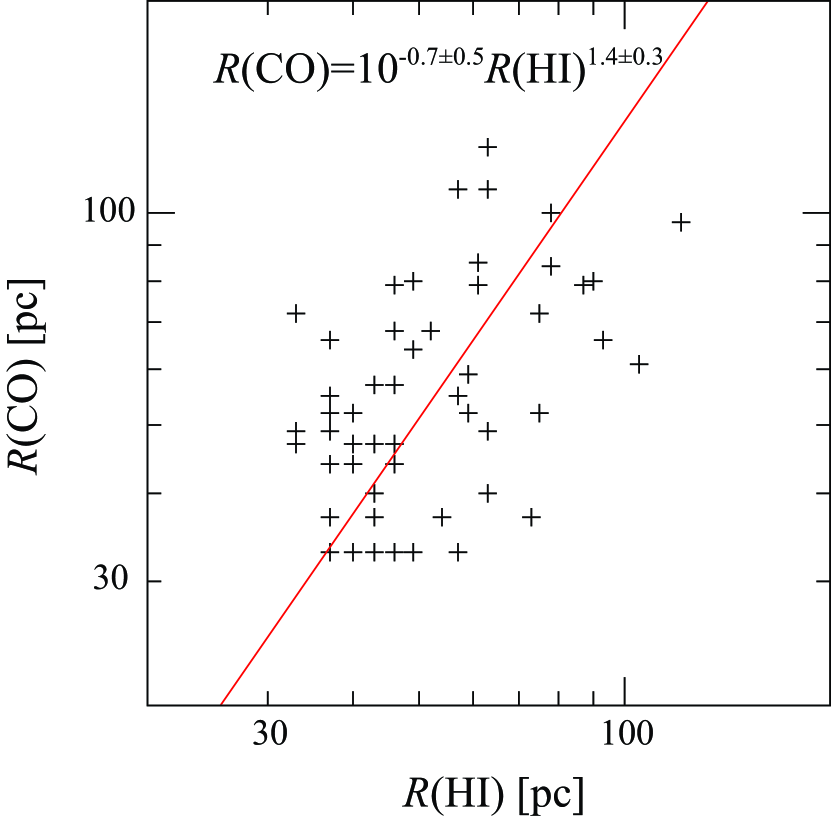
Figure 11: The radius of the GMC, $R$(CO), versus the radius of the HI envelope, $R$(HI) for the 62 clouds with radii greater than 30 pc, as listed in Table 2. The red line is the regression line $R$(CO)$=10^{-0.7\pm 0.5}R$(HI)^1.4±0.3; the Spearman rank correlation coefficient is 0.45.

In Figure 10, we show a histogram of the spatial deviation of the HI and CO peaks. This shows that nearly 80 % of the HI envelopes peak within 120 pc of the local CO peak, and that nearly 60 % of the HI envelopes peak within 80 pc of the CO peak. These separations may seem large compared to $R$(HI), but we argue that they are reasonable if the HI is enveloping CO at scales over $\sim$ 300 pc. It should be noted that the HI envelopes are not concentric with the CO emission, but are rather “enveloping” with some offsets in peak positions as illustrated in Figure 5. We thus expect to find some difference in general between the peak positions of the CO and HI emission (as seen in Figure 10), but the fact that the majority of HI peaks are located within 120 pc of the CO peaks is clearly suggestive of a physical association between the GMCs and their surrounding atomic gas. In Figure 11, we show a correlation between $R$(HI) and $R$(CO) for 62 GMCs whose radius is greater than 30 pc and find that they are positively correlated with a correlation coefficient of 0.45. Despite the relatively flatter distribution of the HI, the size of the HI envelope does seem to correlate with the size of the GMC.

To summarize our analysis in this section, we find for the 123 GMCs with single-peaked HI profiles that: 1) the peak velocities of the CO and HI are in good agreement (Figure 7); 2) the CO and HI linewidths show a positive correlation (Figure 9); 3) the HI envelopes, defined using the 80 % level of the local HI integrated intensity peak, are mostly ($\sim 80$ %) centred within 120 pc of the peak CO position (Figure 10); and 4) the radius of the HI envelope is positively correlated with the size of the GMC for GMCs with radii greater than 30 pc (Figure 11). These four results lend further support to the idea that HI envelopes are physically associated with GMCs, reinforcing the impression conveyed by a global comparison between the HI CO emission in the LMC (Figure 3) and the morphological similarity between the CO and HI in individual velocity channels. (Figure 5).

Next, we made an estimate of the HI column density for the 123 GMCs by using the relation ($N$ (HI) [cm^-2] $=1.8\times 10^{18}\int T_{\rm b}dv$[K km s^-1]). The average values for the three GMC types are listed in Table 1. We find the peak HI column density is mostly in a range of 2–5 $\times 10^{21}$ cm^-2. We estimate the typical density in the HI envelopes to be $\sim 10$ cm^-1 by dividing the peak HI column density 2–5 $\times 10^{21}$ cm^-2 by the typical size of the associated HI 50–100 pc (see Figure 11). The mass of the HI envelopes is large, typically $\sim 5\times 10^{4}M_{\sun}$. The HI envelopes are likely gravitationally bound by GMCs because a half of the HI line width, 7 km s^-1, is nearly equal to $\sqrt{GM/R}\sim 6$ km s^-1 for $M=2\times 10^{5}M_{\sun}$ and $R=40$ pc, the average values of Type II GMCs.

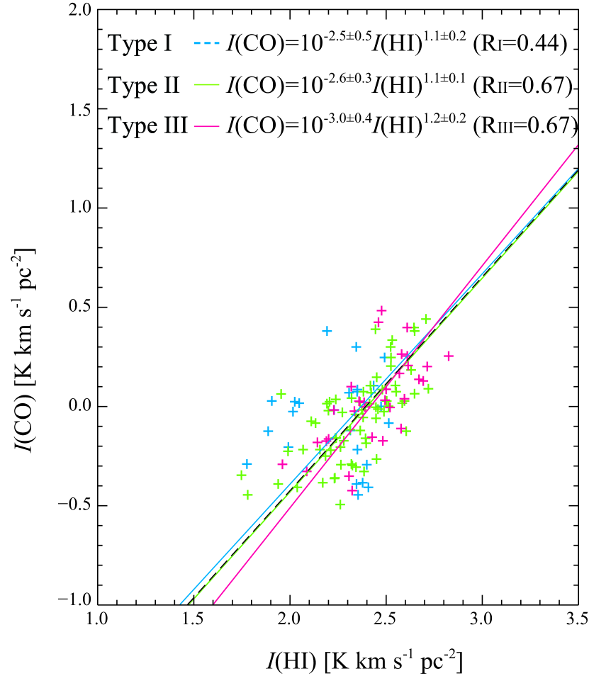
Figure 12: The CO versus HI integrated intensity for the 123 clouds in our sample, averaged over the projected area of each GMC or HI envelope. Blue, green and red plots symbols represent Type I, Type II and Type III GMCs respectively. The black dotted line shows the regression line for all 123 clouds; $I$(CO) $=10^{-2.6\pm 0.2}$$I$(HI)^1.1±0.1. The regression lines and Spearman rank correlation coefficients (R_I, R_II, and R_III) for the three GMC types are shown at the top of the plot.

In Figure 12, we plot the relationship between the average CO and HI luminosity of the 123 GMCs. For each GMC, we selected pixels where CO emission is significantly detected: only these pixels are used to calculate the HI and CO luminosity of each cloud. In order to derive the average CO luminosity of a GMC, we estimated $I$(CO) K km s^-1 by dividing the sum of all the significant CO emission within the GMC by the projected area of the GMC. $I$(HI) K km s^-1 is calculated in a similar manner, summing up the HI emission from the pixels within the GMC with significant CO emission and dividing the result by the area of the GMC. The regression shown in Figure 12 is well fitted by a power law with an index of 1.1, indicating a nearly linear correlation between $I$(CO) and $I$(HI) in a GMC.

4 Discussion

4.1 GMCs with HI envelopes

The present analysis has successfully identified the HI envelopes associated with GMCs on the basis of a 3-D analysis of GMCs in the LMC. The HI intensity in the envelope depends on the star-forming activity within the GMC in the sense that the integrated HI intensity in the envelope increases from Type I to Type III (Figure 4, section 3.1). In other words, massive GMCs have massive HI envelopes and less massive GMCs have less massive HI envelopes.

The HI intensity is a product of the spin temperature and the optical depth of the HI 21 cm transition, provided that the line is optically thin. This is likely to be the case as the HI profiles show few hints of saturation like a flat top. The observed maximum HI brightness temperature is around 100 K and this suggests that the HI spin temperature is significantly higher than 100 K. Therefore we infer that the HI intensity should represent optical depth and, accordingly, HI column density, if the spin temperature is roughly uniform across the LMC. The HI spin temperature in the LMC may be higher than in the Galaxy due to a more intense UV field and the lower dust extinction (Israel 1996; Imara & Blitz 2007; Dobashi et al. 2008). For the sake of discussion, we shall tentatively assume that the spin temperature lies between 150–600 K and is fairly uniform in the HI envelope. We note that the HI mass is accurately determined as long as the HI emission is optically thin. The HI mass does not depend on Ts under the optically thin assumption, because the level populations of the spin doublet having only $\sim 10^{-5}$ eV is well thermalized in any realistic density range due to the slow magnetic dipole decay in $\sim 10^{7}$ yrs.

Fukui et al. (1999) suggest that the three classes of GMC indicate an evolutionary sequence from Type I to Type III in a few 10 Myr (instead of “Type”, these authors used “Class” with the same meaning). Kawamura et al. (2009) present a more detailed analysis of the association between GMCs and young stellar clusters, confirming Fukui et al.’s evolutionary scheme. These studies indicate that only the youngest star clusters with an age less than $\sim 10$ Myr are clearly associated with GMCs, and that older clusters with an age greater than 10 Myr are not associated with GMCs. Assuming a steady state scenario, this implies that the natal gas of clusters is quickly disrupted within 10 Myr. Considering the complete sampling of both clusters and GMCs in the LMC, this strongly suggests that the population of Type III GMCs must be replenished on timescales of 10 Myr. Since the typical time scale of GMC formation is at least 10 Myr, as estimated by the crossing timescale – i.e., the cloud size divided by its velocity dispersion, 100 pc$/$10 km/s $=10$ Myr, a measure of the minimum timescale for GMC formation – we expect to have a similar population of Type III GMCs and Type III precursors. A straightforward interpretation is that Type I and Type II GMCs are these precursors (see for details Kawamura et al. 2009). An alternative possibility is a more ad-hoc situation in which Type III GMCs are formed suddenly in a few Myr by an external disturbance, such as a dynamical interaction. Such a strongly time-dependent scenario seems unlikely, however, since the three GMC types are fairly uniformly distributed over the LMC (Kawamura et al. 2009). Figure 4 of this paper also shows that the three classes of GMCs are distributed across the galaxy.

We have also seen that Type III GMC tend to be more massive than Type I and Type II GMCs (Table 2; Kawamura et al. 2009). A natural interpretation within the evolutionary scenario is that the enveloping HI gas accretes onto a GMC and that the GMC mass increases with time. The accreted HI envelope is converted into H₂ in $\sim 10$ Myr due to increased density, optical extinction and UV shielding. This infall scenario is consistent with the linear relationship between $I$(HI) and $I$(CO) in Figure 12; by contrast, growth of GMCs via collisions between HI clouds would have a steeper relationship, with $I$(CO) proportional to $I$(HI)². For an infall scenario, the infall motion can arise from the gravity of a GMC and possibly from a converging flow driven by super bubbles, while the thermal motion is negligibly small   1.4-3 km s^-1 for kinetic temperatures of $\sim$ 150–600 K. We can roughly estimate the infall velocity to be half of the HI linewidth, i.e. $\sim 7$ km s^-1. This value is consistent with the free fall velocity, $\sim 6$ km s^-1, for a typical Type II GMC. For spherical accretion, where the GMC is surrounded by an HI envelope with a radius of $\sim$40 pc, volume density of $n$(HI) $\sim$10 cm^-3, and an infall speed of $\sim$ 7 km s^-1, we estimate the mass accretion rate to be $\sim$ 0.05 $M_{\sun}$ yr^-1. Over the typical timescale of the GMC evolution, i.e. $\sim$ 10 Myr, the increase in molecular mass amounts to $\sim 5\times 10^{5}M_{\sun}$, which is roughly consistent with the observed typical value for the mass of a Type III GMC ($\sim 4\times 10^{5}M_{\sun}$, Table 1). In the evolutionary picture, the mass accretion of a GMC is terminated by the violent disruption and/or ionization of the molecular material by stellar winds and ionization from young stars.

The infall scenario offers a reasonable interpretation of the HI and CO properties of GMCs that we have explored in this paper. It remains to be seen, however, if an infall velocity field is consistent with 2-D observations; careful analysis of an isolated HI envelope with little kinematical disturbance or nearby contamination could be used to verify this. It is also important to clarify whether the HI linewidth is affected by turbulence to a significant degree.

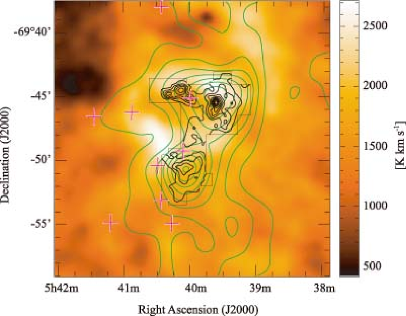
Figure 13: CO and HI emission in the N159 region. The grayscale image represents the combined ATCA+Parkes HI integrated intensity data (Kim et al. 2003). The black contours are integrated CO ($J=$3–2) emission by ASTE (Minamidani et al. 2008) and green contours are integrated CO ($J=$1–0) emission by NANTEN (Fukui et al. 2008). For CO ($J=$3–2), the contour levels are from 5 K km s^-1 in 10 K km s^-1 intervals; for CO ($J=$1–0), the contours levels are from 1.2 K km s^-1 in steps of 2.4 K km s^-1. The thin black lines indicate the region observed in CO ($J=$3–2) emission by ASTE. The crosses indicate the positions of HII regions cataloged by Davies et al. (1976).

It could be argued that the HI gas surrounding GMCs is supplied by the recombination of HII into HI, as both Type II and Type III GMCs are associated with HII regions. This alternative seems unlikely, however: first, the HII regions in Type II GMCs are compact and therefore do not constitute a significant mass reservoir; second, the HI envelope in Type III GMCs are not spatially well-matched with the HII regions and clusters. In N159, for instance, the HII regions and young clusters are confined to the north of the GMC, wherease the HI is more widely distributed in the east and south (Figure 13).

4.2 HI-H₂ conversion in GMCs

This study has shown that the HI and CO distributions correlate well on 40–100 pc scales. It is worth noting, however, that the correlation becomes less clear on smaller scales of $\sim 10$ pc within a GMC. Figure 13 shows an overlay of the HI and CO distributions for the Type III GMC N159, where the CO data was obtained using the ASTE 10 m sub-mm telescope in the ¹²CO $J=$3–2 emission line (Mizuno et al., 2008). Figure 13 shows that the HI becomes less bright at $T_{\rm b}$(HI) 70–80 K toward N159E at (R.A., Dec.)=($5^{\rm h}40^{\rm m}$, $-69\arcdeg,45\arcmin$), compared to intensities of $T_{\rm b}$(HI) $\sim$ 120 K in the HI envelope. A similar behavior was noted by Ott et al. (2008). This is unlikely to be cuased by absorption of the radio continuum emission, as there is no radio continuum emission toward N 159E. We regard this behaviour to be illustrative of the conversion of HI into H₂, as well as the the lower spin temperature in the interior of a GMC. In the inner part of a GMC, HI is converted into H₂ via reactions on grain surfaces on a time scale of $\sim$10 Myr. The HI density is typically $\sim$1 cm^-3, compared to a total molecular density of a few 100 cm^-3, corresponding to atomic to molecular hydrogen ratio of $\sim$100 (e.g., Allen & Robinson 1977; Spitzer 1978; Goldsmith et al. 2007). The spin temperature is also lower, and is likely to equal the molecular gas kinetic temperature of $\sim$ 60 K (e.g., Sato & Fukui 1978; Mizuno et al. 2009). In the HI envelope, on the other hand, the spin temperature is probably between $\sim$ 150-600 K and the HI density is estimated to be $\sim$ 10 cm^-3 with no H₂. The lower $T_{\rm b}$(HI) in the interior is likely due to the lower spin temperature and the lower HI density. The mass of the apparently cold HI gas towards N159E is approximately 10 % of the mass of the HI envelope, $\sim 10^{5}M_{\sun}$, if we assume that the cold HI is optically thin, which suggests that the cold HI within the GMC is not a dominant mass component of the atomic+molecular cloud complex.

It has been shown that there are cold HI components in the LMC as measured from emission and absorption observations toward radio continuum sources (Dickey et al. 1994). These authors detected HI absorption features toward 19 of 30 continuum sources in the LMC and argued that $T_{\rm s}$ of the cold components can be as low as 40 K. Such cold HI components may be associated with GMCs. It is however not clear observationally how the cold HI in absorption is related to GMCs because none of the absorption measurements by Dickey et al (1994) coincide with the NANTEN GMCs.

An issue which has been raised in Wong et al. (2009) is that higher HI intensity is a necessary but not sufficient condition for CO formation. In other words, there are many places with high HI intensities in the LMC without CO. The current analysis has focussed solely on the HI gas surrounding GMCs and therefore does not directly address this issue. We note, however, that it is possible that HI gas with the same intensity can have a significantly different density. We propose an interpretation that the atomic gas in regions with high HI intensities but no CO may have lower densities and higher temperatures. This interpretation could be tested in the future by high velocity-resolution HI observations that can resolve subtle variations in HI profiles and hence identify spatial variations of the atomic gas temperature.

5 Summary

We have carried out the first 3-D analysis of the connection between the CO and HI emission in a galaxy. The major results of our study are as follows:

1. A 3-D comparison at a resolution of 40 pc $\times$ 40 pc $\times$ 1.7 km s^-1 has revealed that the fraction of HI associated with CO tends to increase as a monotonic function of HI intensity without a sharp threshold for the CO formation.

2. We find that GMCs are associated with HI envelopes on scales of $\sim$ 50–100 pc. The HI envelopes have typical volume densities of $\sim$ 10 cm^-3 and an average linewidth of $\sim$14 km s^-1, which is about three times larger than the linewidth of CO. We argue that the HI envelopes are gravitationally bound by GMCs.

3. For 123 GMCs with single-peaked HI profiles, we find a correlation such that [average CO intensity] $\propto$ [average HI intensity]^1.1±0.1. There is a clear increase of the associated HI intensity from GMC Type I to Type III.

4. We interpret our results to mean that a GMC increases in mass via continuous HI accretion over a timescale of $\sim$10 Myr and with a mass accretion rate of 0.05 $M_{\sun}$ yr^-1, before being disrupted by ionization and stellar winds from young clusters. The accreted HI is likely to be converted to molecular hydrogen due to the higher shielding within a GMC.

Table 1: Physical properties of GMCs

GMC Type	Number of	$M_{\rm CO}$	$R$	$N$(HI)	$\Delta V_{\rm LSR}$ (HI)	$\Delta V_{\rm LSR}$ (CO)
	GMCs	($\times 10^{5}M_{\sun}$)	(pc)	($\times 10^{21}$ cm -2)	(km s-1)	(km s-1)
Type I	72	02 (2)	037 (16)	$\cdots$	$\cdots$	05.0 (2.5)
Type II	142	02 (3)	033 (19)	$\cdots$	$\cdots$	04.8 (2.2)
Type III	58	05 (10)	051 (36)	$\cdots$	$\cdots$	06.9 (3.0)
Type I (selected)	24	02 (3)	035 (17)	2.4 (0.9)	013.9 (4.0)	04.5 (2.1)
Type II (selected)	67	02 (3)	041 (22)	2.6 (1.2)	014.6 (4.1)	04.4 (1.6)
Type III (selected)	32	04 (3)	055 (23)	3.3 (1.5)	016.1 (3.3)	05.5 (1.5)

Note. — Average propeties of the GMCs. The values in parentheses are the standard deviation.

Table 2: List of selected 123 GMCs

			peak position(CO)		$R$(CO)	peak position(HI)		$R$(HI)	$N$(HI)	$\sqrt{\Delta\alpha{{}^{2}}+\Delta\delta{{}^{2}}}$
number	name	Type	$\alpha(B1950)$	$\delta(B1950)$	[pc]	$\alpha(B1950)$	$\delta(B1950)$	[pc]	$10^{21}$ [cm${}^{-2}]$	[pc]	comment
1	LMC N J0447-6910	I	$\mathrm{4h47.7m}$	$\mathrm{-69^{\circ}14\arcmin}$	44	$\mathrm{4h47.7m}$	$\mathrm{-69^{\circ}14\arcmin}$	34	2.6	0
4	LMC N J0449-6910	III	$\mathrm{4h49.1m}$	$\mathrm{-69^{\circ}16\arcmin}$	72	$\mathrm{4h49.5m}$	$\mathrm{-69^{\circ}14\arcmin}$	74	2.7	91
5	LMC N J0449-6826	II	$\mathrm{4h49.5m}$	$\mathrm{-68^{\circ}28\arcmin}$	100	$\mathrm{4h50.1m}$	$\mathrm{-68^{\circ}32\arcmin}$	77	1.7	152
9	LMC N J0450-6930	II	$\mathrm{4h50.5m}$	$\mathrm{-69^{\circ}36\arcmin}$	33	$\mathrm{4h50.2m}$	$\mathrm{-69^{\circ}34\arcmin}$	55	2.1	83
11	LMC N J0451-6858	I	$\mathrm{4h51.3m}$	$\mathrm{-69^{\circ}4\arcmin}$	29	$\mathrm{4h51.3m}$	$\mathrm{-69^{\circ}4\arcmin}$	29	2.7	0
12	LMC N J0451-6704	III	$\mathrm{4h51.9m}$	$\mathrm{-67^{\circ}8\arcmin}$	108	$\mathrm{4h52.2m}$	$\mathrm{-67^{\circ}8\arcmin}$	62	3.2	70
17	LMC N J0453-6909	III	$\mathrm{4h54.1m}$	$\mathrm{-69^{\circ}14\arcmin}$	85	$\mathrm{4h53.3m}$	$\mathrm{-69^{\circ}12\arcmin}$	59	2.1	159
22	LMC N J0455-6830	II	$\mathrm{4h55.9m}$	$\mathrm{-68^{\circ}36\arcmin}$	47	$\mathrm{4h55.9m}$	$\mathrm{-68^{\circ}36\arcmin}$	18	2.2	0
23	LMC N J0455-6634	III	$\mathrm{4h56.4m}$	$\mathrm{-66^{\circ}42\arcmin}$	64	$\mathrm{4h56.4m}$	$\mathrm{-66^{\circ}40\arcmin}$	*	1.9	28	30,32,33,236
24	LMC N J0455-6930	III	$\mathrm{4h56.3m}$	$\mathrm{-69^{\circ}36\arcmin}$	29	$\mathrm{4h56.3m}$	$\mathrm{-69^{\circ}36\arcmin}$	18	0.8	0
26	LMC N J0457-6844	III	$\mathrm{4h57.5m}$	$\mathrm{-68^{\circ}48\arcmin}$	29	$\mathrm{4h57.5m}$	$\mathrm{-68^{\circ}48\arcmin}$	24	1.5	0
27	LMC N J0457-6826	III	$\mathrm{4h57.4m}$	$\mathrm{-68^{\circ}30\arcmin}$	40	$\mathrm{4h57.1m}$	$\mathrm{-68^{\circ}32\arcmin}$	18	1.1	91
35	LMC N J0459-6614	II	$\mathrm{4h58.8m}$	$\mathrm{-66^{\circ}18\arcmin}$	79	$\mathrm{4h58.4m}$	$\mathrm{-66^{\circ}24\arcmin}$	85	2.7	130	30,32,33,236
36	LMC N J0500-6622	II	$\mathrm{5h0.7m}$	$\mathrm{-66^{\circ}26\arcmin}$	52	$\mathrm{5h0.7m}$	$\mathrm{-66^{\circ}26\arcmin}$	37	1.5	0
38	LMC N J0502-6903	II	$\mathrm{5h2.4m}$	$\mathrm{-69^{\circ}6\arcmin}$	37	$\mathrm{5h2.4m}$	$\mathrm{-69^{\circ}6\arcmin}$	41	2.1	0
39	LMC N J0503-6553	II	$\mathrm{5h3m}$	$\mathrm{-65^{\circ}58\arcmin}$	40	$\mathrm{5h3m}$	$\mathrm{-65^{\circ}58\arcmin}$	62	2.7	0
40	LMC N J0503-6540	II	$\mathrm{5h3.1m}$	$\mathrm{-65^{\circ}44\arcmin}$	37	$\mathrm{5h3.4m}$	$\mathrm{-65^{\circ}46\arcmin}$	24	0.6	75
41	LMC N J0503-6828	II	$\mathrm{5h3.6m}$	$\mathrm{-68^{\circ}32\arcmin}$	33	$\mathrm{5h4.3m}$	$\mathrm{-68^{\circ}36\arcmin}$	37	1.1	160
43	LMC N J0503-6643	II	$\mathrm{5h3.4m}$	$\mathrm{-66^{\circ}48\arcmin}$	33	$\mathrm{5h3.4m}$	$\mathrm{-66^{\circ}50\arcmin}$	24	1.2	26
45	LMC N J0503-6719	III	$\mathrm{5h3.7m}$	$\mathrm{-67^{\circ}24\arcmin}$	44	$\mathrm{5h3.7m}$	$\mathrm{-67^{\circ}24\arcmin}$	24	2.0	0
46	LMC N J0504-6802	III	$\mathrm{5h4.6m}$	$\mathrm{-68^{\circ}6\arcmin}$	47	$\mathrm{5h4.3m}$	$\mathrm{-68^{\circ}8\arcmin}$	18	1.0	83
48	LMC N J0504-7007	II	$\mathrm{5h5m}$	$\mathrm{-70^{\circ}12\arcmin}$	44	$\mathrm{5h5.1m}$	$\mathrm{-70^{\circ}12\arcmin}$	8	1.4	0
49	LMC N J0504-7056	III	$\mathrm{5h5.3m}$	$\mathrm{-71^{\circ}0\arcmin}$	52	$\mathrm{5h5.3m}$	$\mathrm{-71^{\circ}0\arcmin}$	34	1.0	0
52	LMC N J0506-6753	II	$\mathrm{5h6.8m}$	$\mathrm{-67^{\circ}58\arcmin}$	23	$\mathrm{5h7.2m}$	$\mathrm{-67^{\circ}56\arcmin}$	24	1.0	83
53	LMC N J0507-7041	II	$\mathrm{5h7.9m}$	$\mathrm{-70^{\circ}46\arcmin}$	23	$\mathrm{5h7.8m}$	$\mathrm{-70^{\circ}48\arcmin}$	24	0.9	28
55	LMC N J0507-6858	I	$\mathrm{5h8.1m}$	$\mathrm{-69^{\circ}2\arcmin}$	47	$\mathrm{5h8.1m}$	$\mathrm{-69^{\circ}0\arcmin}$	29	1.3	28
57	LMC N J0508-6905	I	$\mathrm{5h9.1m}$	$\mathrm{-69^{\circ}8\arcmin}$	23	$\mathrm{5h9.2m}$	$\mathrm{-60^{\circ}8\arcmin}$	8	1.0	0
60	LMC N J0509-6827	II	$\mathrm{5h9.4m}$	$\mathrm{-68^{\circ}32\arcmin}$	33	$\mathrm{5h9.5m}$	$\mathrm{-68^{\circ}30\arcmin}$	47	1.6	26
61	LMC N J0509-7049	II	$\mathrm{5h10.2m}$	$\mathrm{-70^{\circ}54\arcmin}$	29	$\mathrm{5h9.8m}$	$\mathrm{-70^{\circ}54\arcmin}$	8	1.0	87
62	LMC N J0509-6912	I	$\mathrm{5h10.2m}$	$\mathrm{-69^{\circ}16\arcmin}$	52	$\mathrm{5h10.6m}$	$\mathrm{-69^{\circ}16\arcmin}$	37	1.7	79
63	LMC N J0510-6853	III	$\mathrm{5h10.4m}$	$\mathrm{-68^{\circ}56\arcmin}$	84	$\mathrm{5h10m}$	$\mathrm{-68^{\circ}52\arcmin}$	77	2.3	93	245,68
64	LMC N J0510-6706	II	$\mathrm{5h10.7m}$	$\mathrm{-67^{\circ}12\arcmin}$	52	$\mathrm{5h11.1m}$	$\mathrm{-66^{\circ}58\arcmin}$	74	1.2	222	67
65	LMC N J0511-6927	II	$\mathrm{5h11.6m}$	$\mathrm{-69^{\circ}30\arcmin}$	23	$\mathrm{5h12m}$	$\mathrm{-69^{\circ}32\arcmin}$	47	0.8	83	244,71
67	LMC N J0512-6710	II	$\mathrm{5h12.1m}$	$\mathrm{-67^{\circ}14\arcmin}$	55	$\mathrm{5h12.4m}$	$\mathrm{-67^{\circ}14\arcmin}$	55	1.6	79	64
68	LMC N J0512-6903	II	$\mathrm{5h12.2m}$	$\mathrm{-69^{\circ}4\arcmin}$	80	$\mathrm{5h11.4m}$	$\mathrm{-69^{\circ}4\arcmin}$	88	1.8	166	63
69	LMC N J0512-7028	II	$\mathrm{5h12.8m}$	$\mathrm{-70^{\circ}32\arcmin}$	68	$\mathrm{5h12.8m}$	$\mathrm{-70^{\circ}30\arcmin}$	50	1.5	26
71	LMC N J0513-6936	II	$\mathrm{5h13.5m}$	$\mathrm{-69^{\circ}40\arcmin}$	79	$\mathrm{5h13.5m}$	$\mathrm{-69^{\circ}44\arcmin}$	59	1.9	62
72	LMC N J0513-6922	III	$\mathrm{5h13.5m}$	$\mathrm{-69^{\circ}26\arcmin}$	49	$\mathrm{5h13.2m}$	$\mathrm{-69^{\circ}24\arcmin}$	34	1.7	83
74	LMC N J0514-7010	II	$\mathrm{5h14.9m}$	$\mathrm{-70^{\circ}14\arcmin}$	66	$\mathrm{5h14.9m}$	$\mathrm{-70^{\circ}14\arcmin}$	34	1.6	0
77	LMC N J0515-7034	I	$\mathrm{5h15.6m}$	$\mathrm{-70^{\circ}38\arcmin}$	44	$\mathrm{5h15.6m}$	$\mathrm{-70^{\circ}38\arcmin}$	18	0.6	0
80	LMC N J0516-6807	II	$\mathrm{5h16.1m}$	$\mathrm{-68^{\circ}2\arcmin}$	124	$\mathrm{5h17.2m}$	$\mathrm{-68^{\circ}4\arcmin}$	62	1.4	237
81	LMC N J0516-6616	I	$\mathrm{5h16m}$	$\mathrm{-66^{\circ}20\arcmin}$	29	$\mathrm{5h16m}$	$\mathrm{-66^{\circ}18\arcmin}$	24	0.3	26
83	LMC N J0516-6922	II	$\mathrm{5h17m}$	$\mathrm{-69^{\circ}26\arcmin}$	23	$\mathrm{5h17.4m}$	$\mathrm{-69^{\circ}26\arcmin}$	34	1.3	87	91
84	LMC N J0516-6559	II	$\mathrm{5h16.7m}$	$\mathrm{-66^{\circ}2\arcmin}$	29	$\mathrm{5h17.1m}$	$\mathrm{-66^{\circ}2\arcmin}$	29	0.6	70
86	LMC N J0517-7114	III	$\mathrm{5h18.3m}$	$\mathrm{-71^{\circ}18\arcmin}$	44	$\mathrm{5h18.3m}$	$\mathrm{-71^{\circ}20\arcmin}$	37	1.3	26
89	LMC N J0517-6642	II	$\mathrm{5h17.6m}$	$\mathrm{-66^{\circ}44\arcmin}$	40	$\mathrm{5h17.6m}$	$\mathrm{-66^{\circ}44\arcmin}$	18	0.9	0
90	LMC N J0517-6932	II	$\mathrm{5h18.5m}$	$\mathrm{-69^{\circ}36\arcmin}$	33	$\mathrm{5h18.5m}$	$\mathrm{-69^{\circ}36\arcmin}$	*	0.9	0
92	LMC N J0518-7001	I	$\mathrm{5h18.8m}$	$\mathrm{-70^{\circ}6\arcmin}$	33	$\mathrm{5h18.1m}$	$\mathrm{-70^{\circ}4\arcmin}$	18	1.1	168
93	LMC N J0518-6620	I	$\mathrm{5h18.3m}$	$\mathrm{-66^{\circ}24\arcmin}$	23	$\mathrm{5h18m}$	$\mathrm{-66^{\circ}22\arcmin}$	*	0.5	75
94	LMC N J0518-6951	II	$\mathrm{5h19.2m}$	$\mathrm{-69^{\circ}54\arcmin}$	23	$\mathrm{5h19.2m}$	$\mathrm{-69^{\circ}56\arcmin}$	24	0.9	26
95	LMC N J0519-6625	I	$\mathrm{5h19m}$	$\mathrm{-66^{\circ}28\arcmin}$	23	$\mathrm{5h19m}$	$\mathrm{-66^{\circ}30\arcmin}$	*	1.2	26	100
96	LMC N J0519-6938	III	$\mathrm{5h19.6m}$	$\mathrm{-69^{\circ}40\arcmin}$	72	$\mathrm{5h19.6m}$	$\mathrm{-69^{\circ}40\arcmin}$	29	2.0	0
97	LMC N J0519-7113	I	$\mathrm{5h20m}$	$\mathrm{-71^{\circ}18\arcmin}$	40	$\mathrm{5h20.4m}$	$\mathrm{-71^{\circ}16\arcmin}$	24	0.9	91
99	LMC N J0520-7043	I	$\mathrm{5h20.4m}$	$\mathrm{-70^{\circ}44\arcmin}$	52	$\mathrm{5h20m}$	$\mathrm{-70^{\circ}46\arcmin}$	37	1.0	91
100	LMC N J0520-665	II	$\mathrm{5h20m}$	$\mathrm{-66^{\circ}54\arcmin}$	37	$\mathrm{5h21m}$	$\mathrm{-66^{\circ}50\arcmin}$	52	1.3	226
103	LMC N J0521-714	II	$\mathrm{5h21.7m}$	$\mathrm{-71^{\circ}46\arcmin}$	23	$\mathrm{5h21.7m}$	$\mathrm{-71^{\circ}46\arcmin}$	24	1.2	0
104	LMC N J0521-701	II	$\mathrm{5h21.6m}$	$\mathrm{-70^{\circ}16\arcmin}$	49	$\mathrm{5h21.2m}$	$\mathrm{-70^{\circ}18\arcmin}$	29	0.8	91
105	LMC N J0521-700	II	$\mathrm{5h21.6m}$	$\mathrm{-70^{\circ}4\arcmin}$	79	$\mathrm{5h21.6m}$	$\mathrm{-70^{\circ}6\arcmin}$	44	1.4	26
106	LMC N J0521-684	II	$\mathrm{5h21.5m}$	$\mathrm{-68^{\circ}44\arcmin}$	29	$\mathrm{5h21.5m}$	$\mathrm{-68^{\circ}44\arcmin}$	8	1.7	0
108	LMC N J0521-684	II	$\mathrm{5h21.8m}$	$\mathrm{-68^{\circ}50\arcmin}$	55	$\mathrm{5h21.8m}$	$\mathrm{-68^{\circ}50\arcmin}$	34	1.4	0
110	LMC N J0522-694	III	$\mathrm{5h22.7m}$	$\mathrm{-69^{\circ}44\arcmin}$	52	$\mathrm{5h22.3m}$	$\mathrm{-69^{\circ}44\arcmin}$	18	1.2	79
115	LMC N J0522-654	III	$\mathrm{5h22.6m}$	$\mathrm{-65^{\circ}44\arcmin}$	57	$\mathrm{5h22.6m}$	$\mathrm{-65^{\circ}42\arcmin}$	44	1.7	26
118	LMC N J0523-682	I	$\mathrm{5h22.9m}$	$\mathrm{-68^{\circ}24\arcmin}$	44	$\mathrm{5h22.9m}$	$\mathrm{-68^{\circ}26\arcmin}$	37	3.2	26
119	LMC N J0523-664	II	$\mathrm{5h23m}$	$\mathrm{-66^{\circ}46\arcmin}$	57	$\mathrm{5h22.7m}$	$\mathrm{-66^{\circ}46\arcmin}$	41	2.5	79
123	LMC N J0523-713	II	$\mathrm{5h24.2m}$	$\mathrm{-71^{\circ}42\arcmin}$	49	$\mathrm{5h26.4m}$	$\mathrm{-71^{\circ}38\arcmin}$	62	1.4	466	131,249
126	LMC N J0524-672	II	$\mathrm{5h24.5m}$	$\mathrm{-67^{\circ}30\arcmin}$	44	$\mathrm{5h24.5m}$	$\mathrm{-67^{\circ}30\arcmin}$	24	2.3	0
127	LMC N J0524-702	I	$\mathrm{5h24.8m}$	$\mathrm{-70^{\circ}30\arcmin}$	37	$\mathrm{5h24.4m}$	$\mathrm{-70^{\circ}30\arcmin}$	24	0.6	87
130	LMC N J0524-691	II	$\mathrm{5h24.9m}$	$\mathrm{-69^{\circ}18\arcmin}$	33	$\mathrm{5h24.5m}$	$\mathrm{-69^{\circ}12\arcmin}$	47	1.2	123
131	LMC N J0524-713	II	$\mathrm{5h25.5m}$	$\mathrm{-71^{\circ}36\arcmin}$	29	$\mathrm{5h25.9m}$	$\mathrm{-71^{\circ}38\arcmin}$	64	1.7	99	123,249
132	LMC N J0525-694	II	$\mathrm{5h26.2m}$	$\mathrm{-69^{\circ}52\arcmin}$	33	$\mathrm{5h25.8m}$	$\mathrm{-69^{\circ}56\arcmin}$	34	1.0	99
133	LMC N J0525-691	III	$\mathrm{5h26m}$	$\mathrm{-69^{\circ}20\arcmin}$	33	$\mathrm{5h24.5m}$	$\mathrm{-69^{\circ}12\arcmin}$	47	0.8	359	130
134	LMC N J0525-662	II	$\mathrm{5h25.7m}$	$\mathrm{-66^{\circ}24\arcmin}$	23	$\mathrm{5h25.3m}$	$\mathrm{-66^{\circ}26\arcmin}$	116	3.8	75	135
136	LMC N J0526-683	II	$\mathrm{5h26.2m}$	$\mathrm{-68^{\circ}38\arcmin}$	37	$\mathrm{5h26.2m}$	$\mathrm{-68^{\circ}38\arcmin}$	41	1.4	0
139	LMC N J0526-684	III	$\mathrm{5h26.6m}$	$\mathrm{-68^{\circ}50\arcmin}$	29	$\mathrm{5h26.3m}$	$\mathrm{-68^{\circ}48\arcmin}$	29	1.9	91
141	LMC N J0526-655	II	$\mathrm{5h26.5m}$	$\mathrm{-65^{\circ}56\arcmin}$	23	$\mathrm{5h26.2m}$	$\mathrm{-66^{\circ}0\arcmin}$	160	2.0	93	134,135,250
143	LMC N J0526-711	II	$\mathrm{5h27.5m}$	$\mathrm{-71^{\circ}22\arcmin}$	97	$\mathrm{5h26m}$	$\mathrm{-71^{\circ}26\arcmin}$	120	1.3	346	153,156
145	LMC N J0527-703	II	$\mathrm{5h28m}$	$\mathrm{-70^{\circ}38\arcmin}$	40	$\mathrm{5h28.1m}$	$\mathrm{-70^{\circ}40\arcmin}$	18	0.6	26
146	LMC N J0527-705	II	$\mathrm{5h28.6m}$	$\mathrm{-70^{\circ}54\arcmin}$	37	$\mathrm{5h28.6m}$	$\mathrm{-70^{\circ}54\arcmin}$	72	1.0	0	149
149	LMC N J0528-705	II	$\mathrm{5h29m}$	$\mathrm{-71^{\circ}0\arcmin}$	33	$\mathrm{5h29.4m}$	$\mathrm{-71^{\circ}0\arcmin}$	24	1.7	87
150	LMC N J0529-683	II	$\mathrm{5h30.2m}$	$\mathrm{-68^{\circ}32\arcmin}$	29	$\mathrm{5h30.6m}$	$\mathrm{-68^{\circ}36\arcmin}$	142	1.8	106	154,163
153	LMC N J0530-710	III	$\mathrm{5h31.6m}$	$\mathrm{-71^{\circ}10\arcmin}$	80	$\mathrm{5h31.6m}$	$\mathrm{-71^{\circ}10\arcmin}$	47	2.6	0
154	LMC N J0531-683	III	$\mathrm{5h31.7m}$	$\mathrm{-68^{\circ}34\arcmin}$	108	$\mathrm{5h32.7m}$	$\mathrm{-68^{\circ}28\arcmin}$	55	2.7	243	150,163
155	LMC N J0532-674	III	$\mathrm{5h32m}$	$\mathrm{-67^{\circ}46\arcmin}$	68	$\mathrm{5h32.7m}$	$\mathrm{-67^{\circ}46\arcmin}$	44	3.1	157
156	LMC N J0532-711	II	$\mathrm{5h32.9m}$	$\mathrm{-71^{\circ}16\arcmin}$	47	$\mathrm{5h32.9m}$	$\mathrm{-71^{\circ}16\arcmin}$	41	2.5	0
157	LMC N J0532-683	II	$\mathrm{5h32.5m}$	$\mathrm{-68^{\circ}40\arcmin}$	40	$\mathrm{5h32.5m}$	$\mathrm{-68^{\circ}40\arcmin}$	41	2.7	0
158	LMC N J0532-662	III	$\mathrm{5h32.4m}$	$\mathrm{-66^{\circ}30\arcmin}$	47	$\mathrm{5h32m}$	$\mathrm{-66^{\circ}26\arcmin}$	29	0.9	99
162	LMC N J0532-685	II	$\mathrm{5h33.4m}$	$\mathrm{-69^{\circ}0\arcmin}$	33	$\mathrm{5h33m}$	$\mathrm{-69^{\circ}0\arcmin}$	18	2.4	79
171	LMC N J0535-690	III	$\mathrm{5h36m}$	$\mathrm{-69^{\circ}4\arcmin}$	66	$\mathrm{5h36.4m}$	$\mathrm{-69^{\circ}4\arcmin}$	91	3.5	79	183
172	LMC N J0535-684	II	$\mathrm{5h36.2m}$	$\mathrm{-68^{\circ}46\arcmin}$	37	$\mathrm{5h35.8m}$	$\mathrm{-68^{\circ}46\arcmin}$	41	1.6	79
179	LMC N J0537-661	III	$\mathrm{5h37.3m}$	$\mathrm{-66^{\circ}20\arcmin}$	47	$\mathrm{5h37.3m}$	$\mathrm{-66^{\circ}20\arcmin}$	44	2.1	0
180	LMC N J0537-662	II	$\mathrm{5h37.4m}$	$\mathrm{-66^{\circ}28\arcmin}$	23	$\mathrm{5h37.1m}$	$\mathrm{-66^{\circ}30\arcmin}$	34	1.8	75
184	LMC N J0538-693	II	$\mathrm{5h38.7m}$	$\mathrm{-69^{\circ}36\arcmin}$	33	$\mathrm{5h39.1m}$	$\mathrm{-69^{\circ}34\arcmin}$	41	3.5	83	191
190	LMC N J0538-685	III	$\mathrm{5h38.9m}$	$\mathrm{-68^{\circ}56\arcmin}$	23	$\mathrm{5h41.1m}$	$\mathrm{-68^{\circ}54\arcmin}$	81	2.9	480
191	LMC N J0539-693	III	$\mathrm{5h39.4m}$	$\mathrm{-69^{\circ}32\arcmin}$	57	$\mathrm{5h39.1m}$	$\mathrm{-69^{\circ}34\arcmin}$	41	3.5	83	184
205	LMC N J0542-711	III	$\mathrm{5h42.1m}$	$\mathrm{-71^{\circ}20\arcmin}$	64	$\mathrm{5h42m}$	$\mathrm{-71^{\circ}18\arcmin}$	47	2.5	28
207	LMC N J0542-694	II	$\mathrm{5h43.5m}$	$\mathrm{-69^{\circ}46\arcmin}$	23	$\mathrm{5h43.5m}$	$\mathrm{-69^{\circ}46\arcmin}$	18	4.1	0	266
208	LMC N J0543-675	III	$\mathrm{5h43.5m}$	$\mathrm{-67^{\circ}58\arcmin}$	37	$\mathrm{5h43.8m}$	$\mathrm{-67^{\circ}58\arcmin}$	34	2.0	79	211
209	LMC N J0543-692	II	$\mathrm{5h43.9m}$	$\mathrm{-69^{\circ}28\arcmin}$	33	$\mathrm{5h44.2m}$	$\mathrm{-69^{\circ}22\arcmin}$	47	3.0	106	214,216,268
211	LMC N J0543-675	III	$\mathrm{5h43.8m}$	$\mathrm{-67^{\circ}56\arcmin}$	23	$\mathrm{5h43.8m}$	$\mathrm{-67^{\circ}58\arcmin}$	29	1.8	28	208
214	LMC N J0543-691	II	$\mathrm{5h43.4m}$	$\mathrm{-69^{\circ}16\arcmin}$	33	$\mathrm{5h44.2m}$	$\mathrm{-69^{\circ}22\arcmin}$	44	2.5	211	209,216,268
215	LMC N J0544-712	I	$\mathrm{5h45.2m}$	$\mathrm{-71^{\circ}28\arcmin}$	59	$\mathrm{5h44.7m}$	$\mathrm{-71^{\circ}28\arcmin}$	57	1.9	87
218	LMC N J0544-671	II	$\mathrm{5h44.9m}$	$\mathrm{-67^{\circ}20\arcmin}$	29	$\mathrm{5h44.4m}$	$\mathrm{-67^{\circ}28\arcmin}$	50	1.0	167	213
220	LMC N J0545-694	III	$\mathrm{5h45.9m}$	$\mathrm{-69^{\circ}50\arcmin}$	47	$\mathrm{5h45.6m}$	$\mathrm{-69^{\circ}52\arcmin}$	37	2.0	83
222	LMC N J0546-710	I	$\mathrm{5h46.8m}$	$\mathrm{-71^{\circ}6\arcmin}$	44	$\mathrm{5h46.8m}$	$\mathrm{-71^{\circ}6\arcmin}$	44	1.7	0
223	LMC N J0546-693	II	$\mathrm{5h46.8m}$	$\mathrm{-69^{\circ}38\arcmin}$	52	$\mathrm{5h47.2m}$	$\mathrm{-69^{\circ}40\arcmin}$	57	3.3	99
224	LMC N J0547-680	I	$\mathrm{5h47.6m}$	$\mathrm{-68^{\circ}10\arcmin}$	33	$\mathrm{5h48m}$	$\mathrm{-68^{\circ}10\arcmin}$	55	1.7	79
225	LMC N J0547-704	I	$\mathrm{5h47.8m}$	$\mathrm{-70^{\circ}42\arcmin}$	87	$\mathrm{5h47.8m}$	$\mathrm{-70^{\circ}40\arcmin}$	*	1.3	28	228
226	LMC N J0547-6953	II	$\mathrm{5h48.7m}$	$\mathrm{-69^{\circ}54\arcmin}$	61	$\mathrm{5h48m}$	$\mathrm{-69^{\circ}56\arcmin}$	104	1.6	159	223,227,270
230	LMC N J0555-681	III	$\mathrm{5h55.9m}$	$\mathrm{-68^{\circ}10\arcmin}$	73	$\mathrm{5h55.9m}$	$\mathrm{-68^{\circ}10\arcmin}$	*	1.3	0	271
231	LMC N J0447-672	I	$\mathrm{4h47.2m}$	$\mathrm{-67^{\circ}34\arcmin}$	17	$\mathrm{4h47.1m}$	$\mathrm{-67^{\circ}36\arcmin}$	190	1.2	28	2,232
232	LMC N J0448-672	I	$\mathrm{4h48m}$	$\mathrm{-67^{\circ}28\arcmin}$	17	$\mathrm{4h47.2m}$	$\mathrm{-67^{\circ}18\arcmin}$	82	1.2	229	2
233	LMC N J0449-681	II	$\mathrm{4h49.8m}$	$\mathrm{-68^{\circ}16\arcmin}$	17	$\mathrm{4h49.5m}$	$\mathrm{-68^{\circ}12\arcmin}$	88	1.3	86	6
236	LMC N J0458-661	II	$\mathrm{4h58.7m}$	$\mathrm{-66^{\circ}22\arcmin}$	17	$\mathrm{4h58.4m}$	$\mathrm{-66^{\circ}24\arcmin}$	75	3.7	83	30,32,33,35
237	LMC N J0459-660	II	$\mathrm{4h59.8m}$	$\mathrm{-66^{\circ}12\arcmin}$	17	$\mathrm{5h0.2m}$	$\mathrm{-66^{\circ}12\arcmin}$	*	2.7	70
243	LMC N J0511-705	I	$\mathrm{5h12.3m}$	$\mathrm{-70^{\circ}54\arcmin}$	17	$\mathrm{5h12.7m}$	$\mathrm{-70^{\circ}54\arcmin}$	8	0.7	87
244	LMC N J0511-692	II	$\mathrm{5h12m}$	$\mathrm{-69^{\circ}32\arcmin}$	17	$\mathrm{5h12m}$	$\mathrm{-69^{\circ}32\arcmin}$	29	1.1	0	65
247	LMC N J0521-673	I	$\mathrm{5h21.8m}$	$\mathrm{-67^{\circ}42\arcmin}$	17	$\mathrm{5h22.1m}$	$\mathrm{-67^{\circ}36\arcmin}$	34	0.9	117
252	LMC N J0528-672	III	$\mathrm{5h28m}$	$\mathrm{-67^{\circ}28\arcmin}$	17	$\mathrm{5h28m}$	$\mathrm{-67^{\circ}28\arcmin}$	29	2.3	0
253	LMC N J0530-675	I	$\mathrm{5h30.7m}$	$\mathrm{-68^{\circ}0\arcmin}$	17	$\mathrm{5h31m}$	$\mathrm{-67^{\circ}58\arcmin}$	47	2.1	83
258	LMC N J0535-661	II	$\mathrm{5h35.3m}$	$\mathrm{-66^{\circ}20\arcmin}$	17	$\mathrm{5h35.3m}$	$\mathrm{-66^{\circ}18\arcmin}$	24	0.7	28
266	LMC N J0543-694	II	$\mathrm{5h43.6m}$	$\mathrm{-69^{\circ}48\arcmin}$	17	$\mathrm{5h43.5m}$	$\mathrm{-69^{\circ}46\arcmin}$	18	3.6	28	207
270	LMC N J0547-695	II	$\mathrm{5h48.1m}$	$\mathrm{-70^{\circ}0\arcmin}$	17	$\mathrm{5h48.6m}$	$\mathrm{-70^{\circ}6\arcmin}$	82	2.0	143	226,227
271	LMC N J0553-682	I	$\mathrm{5h53.3m}$	$\mathrm{-68^{\circ}24\arcmin}$	17	$\mathrm{5h53.3m}$	$\mathrm{-68^{\circ}24\arcmin}$	55	1.9	0

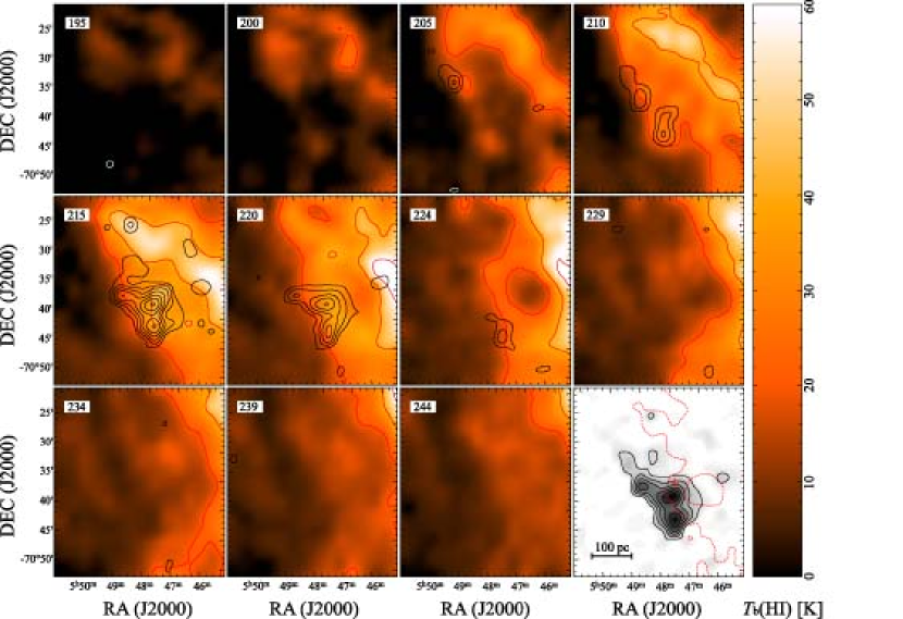
Figure 5: Velocity channel maps of the HI and CO emission associated with Type I, Type II, and Type III, GMCs. The grayscale images with black contours are HI brightness temperature (Kim et al. 2003) and the white contours are CO intensity (Fukui et al. 2008). The central velocity of the included channels is shown in the upper left of each panel. The lower right panel of each figure shows the total CO integrated intensity. The red contours and the red cross in the lower right panel of (a) and (b) present the 80 % level of the HI peak intensity and the position of the HI intensity peak, respectively. (a) GMC no. 225 in the NANTEN catalog. CO contour levels are from 0.105 K km s^-1 ($3\sigma$) with 0.105 K km s^-1 intervals. HI contour levels are from 20 K with 20 K intervals. This is a case where the 80 % level of the HI peak intensity is very extended relative to the size of the GMC. (b) GMC no. 134 and 135 between LMC4 and LMC5. CO integrated intensities are from 0.105 K km s^-1 with 0.105 K km s^-1 intervals. HI contour levels are from 20 K with 20 K intervals. This is a case where the 80 % of the HI peak intensity provides a sensible definition of the HI envelope size. (c) GMC no. 192 and 202 with the HII region N159. CO integrated intensities are from 0.105 K km s^-1 with 0.21 K km s^-1 ($6\sigma$) intervals. HI contour levels are from 20 K with 20 K intervals. This is a region where the HI emission is very complicated; it was not selected in the sample of 123 clouds that we use for our analysis.

Fig. 5(b). — continued

Fig. 5(c). — continued

References

- (1) Allen, M., & Robinson, G. W., 1977, ApJ, 212, 396
- (2) Andersson, B.-G., Wannier, P. G., & Morris, M., ApJ, 1991, 366, 464
- (3) Bica, E., Claria, J. J., Dottori, H., Santos, J. F. C. Jr., & Piatti, A. E., 1996, ApJS, 102, 57
- (4) Blitz, L., Fukui, Y., Kawamura, A. Leroy, A., Mizuno, N., & Rosolowsky, E. 2007, in Protostars and Planet V, ed. B. Reipurth, D. Jewitt, & K. Keil (University of Arizona) 951
- (5) Davies, R. D., Elliott, K. H., & Meaburn, J. 1976, MmRAS, 81, 89
- Dickey et al (1994) Dickey, J. M., Mebold, U., Marx, M., Amy, S., Haynes, R. F., Wilson, W. 1994, A&A, 289, 357
- Dobashi et al. (1996) Dobashi, K., Bernard, J. P., Hughes, A., Paradis, D., Reach, W. T., & Kawamura, A. 2008, A&A, 484, 205
- Fukui (2007) Fukui, Y. 2007, in IAU Symp. 237, Triggered Star Formation in a Turbulent ISM, ed. B. Elmegreen & J. Palous (Cambridge), 31
- Fukui et al. (1999) Fukui, Y., Mizuno, N., Yamaguchi, R., Mizuno, A., Onishi, T., Ogawa, H., Yonekura, Y., Kawamura, A., Tachihara, K., Xiao, K., et al. 1999, PASJ, 51, 745
- Fukui (2008) Fukui, Y., et al. 2008, ApJS, 178, 56
- Haynes et al. (1991) Goldsmith, P., Li, & D., Krco, M. 2007, ApJ, 654, 273
- Heyer et al. (2001) Hasegawa, T., Sato, F., & Fukui, Y. 1983, AJ, 88, 658
- hughes (06) Imara, N., & Blitz, L.,2007, ApJ, 662, 969
- i (2) Israel, F. P., Maloney, P. R., Geis, N., Herrmann, F., Madden, S. C., Poglitsch, A., & Stacey, G. J. 1996, ApJ, 465, 738
- kawamura (2008) Kawamura, A., et al. 2009, ApJS, 184, 1
- i (2) Kennicutt, R. C. Jr. 1988, ApJ, 498, 541
- (17) Kim, S., Dopita, M. A., Staveley-Smith, L., & Bessel, M. S. 1999, AJ, 118, 2797
- Kim (03) Kim, S., Staveley-Smith, L., Dopita, M. A., Sault, R. J., Freeman, K. C., Lee, Y., Chu, Y.-H. 2003, ApJ, 148, 473
- Meixner et al. (2006) Minamidani, T., et al. 2008, ApJS, 175, 485
- m (1) Mizuno, N., Muller, E., Maeda, H., Kawamura, A., Minamidani, T., Onishi, T., Mizuno, A., & Fukui, Y., 2006, ApJ, 643, 107
- m (2) Mizuno, N., Rubio, M., Mizuno, A., Yamaguchi, R., Onishi, T., Fukui, Y. 2001, PASJ, 53, L45
- m (3) Mizuno, Y., et al. 2009, PASJ, submitted
- m (1) Ott, J., et al. 2008, PASA, 25, 129
- Nakagawa et al. (2005) Sato, F., & Fukui, Y. 1978, AJ, 83, 1607
- Ogawa et al. (1987) Schmidt,Th. 1972, A&A, 16, 95
- (26) Spitzer, L. Jr.1978, Physical Processes in the Interstellar Medium (New York: Wiley Interscience)
- Solomon et al. (1987) Wannier, P. G., Lichten, S.M., & Morris, M., 1983, Ap.J., 268, 727
- Wong & Blitz (2002) Wong, T., et al. 2009, ApJ, 696, 370 (Paper I)
- y (2) Yamaguchi, R., et al. 2001, PASJ, 53, 9