Experimental consistency in parton distribution fitting

Abstract

The recently developed “Data Set Diagonalization” method (DSD) is applied to measure compatibility of the data sets that are used to determine parton distribution functions (PDFs). Discrepancies among the experiments are found to be somewhat larger than is predicted by propagating the published experimental errors according to Gaussian statistics. The results support a tolerance criterion of $\Delta\chi^{2}\approx 10$ to estimate the 90% confidence range for PDF uncertainties. No basis is found in the data sets for the much larger $\Delta\chi^{2}$ values that are in current use; though it will be necessary to retain those larger values until improved methods can be developed to take account of systematic errors in applying the theory. The DSD method also measures how much influence each experiment has on the global fit, and identifies experiments that show significant tension with respect to the others. The method is used to explore the contribution from muon scattering experiments, which are found to exhibit the largest discrepancies in the current fit.

I Introduction

Interactions at high energy colliders such as the Tevatron and LHC are interpreted according to Quantum Chromodynamics (QCD) and Electroweak theory on the basis of collisions between partons. The analysis of collider data therefore relies on knowing the parton distribution functions (PDFs) that describe probability densities for the gluon ($g$) and quark partons ($u$, $d$, $c$, $s$, $b$) and their antiquarks ($\bar{u}$, $\bar{d}$, $\bar{c}$, $\bar{s}$, $\bar{b}$) in the proton, as a function of momentum fraction $x$ and QCD factorization scale $\mu$. In keeping with their importance, there is a sizeable industry in attempting to determine the PDFs cteq60 ; cteq66 ; CT09 ; MSTW08 ; NNPDF .

An integral part of the PDF effort is the need to estimate the uncertainty of the results. An obvious component of that uncertainty comes from the reported errors in the data. It has become standard practice cteq66 ; CT09 ; MSTW08 to inflate the uncertainties obtained in this way, motivated in part by a notion that disagreements between different experiments in the global fit signal the presence of unknown systematic errors in the experiments—or else they indicate important systematic errors in the theory, which could for example be introduced by the perturbative approximations to QCD.

The recently-invented method of Data Set Diagonalization (DSD) DSD offers a direct assessment of the contribution from each experiment to the global fit, and provides a statistical measure of the consistency between each experiment and the others. The method was illustrated in DSD by applying it to three of the experiments in a contemporary PDF analysis CT09 . That study is extended in this paper to systematically examine the contribution and consistency of every experiment in the analysis.

The DSD study is important for two reasons. First, the overall level of consistency among the experiments provides quantitative information on how to assign uncertainty estimates to predictions based on the global fit. Second, the study identifies experiments whose implications are in disagreement with the consensus of the others, due to unknown theoretical or experimental problems.

II The PDF fitting paradigm

In current practice, one attempts to determine $u(x)$, $\bar{u}(x)$, $d(x)$, $\bar{d}(x)$, $s(x)$, $\bar{s}(x)$, $g(x)$ at some low QCD scale $\mu_{0}$. The distributions at all higher scales are then given by the QCD renormalization group DGLAP equations. The $c$ and $b$ distributions are generally assumed to arise only from this perturbatively calculable evolution in $\mu$; and available data are consistent with $s(x)=\bar{s}(x)$. This leaves 6 unknown functions of $x$ to be determined from experiment. These functions are further constrained theoretically only by the number sum rules $\int_{0}^{1}\,(u(x)-\bar{u}(x))\,dx=2$ and $\int_{0}^{1}\,(d(x)-\bar{d}(x))\,dx=1$, the momentum sum rule, some theoretical predictions on limiting behavior at $x\to 0$ and $x\to 1$, positivity, and notions of expected smoothness.

In the paradigm used here, the parton distributions at $\mu_{0}$ are expressed as functional forms in $x$, with a large number of adjustable parameters. The parameter values are determined by a “global analysis” in which data from a wide variety of experiments are fitted simultaneously. No single experiment directly measures any one the basic distributions; but the workings of QCD tie each data point to a different convolution integral over the distributions, and hence to a different combination of the unknown parameters.

III The DSD method

This Section summarizes the DSD method DSD . As a further aid to understanding it, the method is illustrated in the Appendix by a simple explicit example.

The $\chi^{2}$ measure of the quality of fit to the full body of data is a function of parameters $a_{1}$,…,$\,a_{n}$ that define the parton distributions at scale $\mu_{0}$ (here $n=24$ and $\mu_{0}=1.4\,\mathrm{GeV}$). The best-fit PDF set is found by minimizing $\chi^{2}$ with respect to those parameters. The uncertainty range of the fit is estimated as the region in parameter space that is sufficiently close to this minimum: $\chi^{2}\,\leq\,\chi_{\mathrm{min}}^{2}\,+\,\Delta\chi^{2}\,$.

The dependence of $\chi^{2}$ on $\{a_{i}\}$ can be expanded about the minimum through second order using Taylor series. The eigenvectors of the quadratic form that governs that expansion can be used as basis vectors to obtain a linear transformation to new coordinates for which

$$\chi^{2}\,=\,\chi_{\mathrm{min}}^{\,2}\,+\,\sum_{i=1}^{n}y_{i}^{\,2}\;.$$ (1)

This is known as the Hessian method Hessian . The DSD method DSD builds upon it by simultaneously diagonalizing $\chi^{2}$ and the contribution to $\chi^{2}$ from a subset of the data, such as a single one of the experiments. This is done as follows. Let $\chi_{\mathbf{S}}^{\,2}$ be the contribution to $\chi^{2}$ from the subset. In the neighborhood of the global minimum, $\chi_{\mathbf{S}}^{\,2}$ can be expanded through second order in the coordinates $\{y_{i}\}$ by again using Taylor series. The eigenvectors of the second-derivative matrix which appears in that expansion provide a further linear transformation which diagonalizes its quadratic form, without spoiling Eq. (1). Combining the two linear transformations yields a single linear transformation of the fitting parameters $\{a_{i}\}$ to new parameters $\{z_{i}\}$ for which

$$\chi^{\,2} = \chi_{\mathbf{S}}^{\,2}\,+\,\chi_{\mathbf{\overline{S}}}^{\,2}\,=\,\sum_{i=1}^{n}z_{i}^{\,2}$$ (2)

$$\chi_{\mathbf{S}}^{\,2} = \sum_{i=1}^{n}\gamma_{i}\,(z_{i}-A_{i})^{2}\,+\,\mathrm{const}$$ (3)

$$\chi_{\mathbf{\overline{S}}}^{\,2} = \sum_{i=1}^{n}\,(1-\gamma_{i})\,(z_{i}-C_{i})^{2}\,+\,\mathrm{const}\;,$$ (4)

where $\,\gamma_{i}A_{i}\,+\,(1-\gamma_{i})C_{i}\,=\,0$. Assuming that $0<\gamma_{i}<1$, Eqs. (3–4) can be written in the form

$$\chi_{\mathbf{S}}^{\,2} = \sum_{i=1}^{n}\left(\frac{z_{i}-A_{i}}{B_{i}}\right)^{2}\,+\,\mathrm{const}$$

$$\chi_{\mathbf{\overline{S}}}^{\,2} = \sum_{i=1}^{n}\left(\frac{z_{i}-C_{i}}{D_{i}}\right)^{2}\,+\,\mathrm{const}\;,$$ (5)

which cries out to be be interpreted as independent measurements:

$$\mbox{$\mathbf{S}$:}\;\;z_{i} = A_{i}\,\pm\,B_{i}$$

$$\mbox{$\mathbf{\overline{S}}$:}\;\;z_{i} = C_{i}\,\pm\,D_{i}\;.$$ (6)

The parameters $\gamma_{i}$ determine the precision of these measurements through

$$B_{i} = 1/\sqrt{\gamma_{i}}$$

$$D_{i} = 1/\sqrt{1-\gamma_{i}}\;.$$ (7)

In the PDF analysis, the largest values of $\gamma_{i}$ that appear are $\,\sim\!0.9\,$. Most of the $\gamma_{i}$ are smaller than that, since most properties of the global fit are significantly constrained by more than one experiment—both because different kinds of experiments are strongly linked by QCD, and because many of the key measurements have been made more than once (often by more than one experimental group). The study in Sec. IV reports all of the results with $\gamma_{i}\geq 0.1$. Directions for which $\gamma_{i}<0.1$ can be neglected, since for these directions, the uncertainty of $\mathbf{S}$ is at least 3 times larger than the uncertainty from the other experiments, so it contributes little to the weighted average. In practice some $\gamma_{i}$ even come out negative. When that happens, it indicates that $\mathbf{S}$ is so insensitive to $z_{i}$ in the allowed range $|z_{i}|\lesssim 1$ that the quadratic approximation has broken down for that experiment along that direction. Since $\mathbf{S}$ is insensitive to $z_{i}$ along such directions, it is correct to ignore them along with the other directions for which $\gamma_{i}<0.1\,$.

The new coordinates are chosen such that the average of the two measurements (6), weighted by their uncertainties, gives

$$z_{i}=0\,\pm\,1$$ (8)

according to Eq. (2). The difference between the two measurements (6) provides a direct measure of the consistency between $\mathbf{S}$ and its complement $\mathbf{\overline{S}}$. That difference can be expressed in standard deviations as

$$\sigma_{i}\,=\,\frac{|A_{i}-C_{i}|}{\sqrt{B_{i}^{\,2}+D_{i}^{\,2}}}\,=\,\sqrt{\gamma_{i}\,(1-\gamma_{i})}\,|A_{i}-C_{i}|\;.$$ (9)

The parameter $\gamma_{i}$ characterizes the importance of experiment $\mathbf{S}$, while the parameter $\sigma_{i}$ characterizes its consistency with $\mathbf{\overline{S}}$, along direction $z_{i}$. In the next Section, these key parameters are evaluated for every experiment in the PDF global fit.

IV Results from the DSD method

We study a body of input data that is nearly the same as was used in the recent CT09 analysis CT09 . The parametrization of the PDFs is identical to CT09, with the same 24 free parameters. The definition of $\chi^{2}$ used here is just the sum over data points of ((data-theory)/error)², except for including correlated systematic experimental errors for all data sets for which these have been published. Unlike in CT09, no weight factors or penalties are applied in $\chi^{2}$ to emphasize particular experiments.

Process	Expt	N	$\sum_{i}\gamma_{i}$	$(\gamma_{1},\,\sigma_{1}),\,(\gamma_{2},\,\sigma_{2}),\,\dots$
$e^{+}\,p\to e^{+}\,X$	H1 NC Adloff:2000qk	115	2.10	$(0.72,\,0.01)$ $(0.59,\,\mathbf{3.02})$ $(0.43,\,0.20)$ $(0.36,\,1.37)$
$e^{-}\,p\to e^{-}\,X$	H1 NC Adloff:2000qj	126	0.30	$(0.30,\,0.02)$
$e^{+}\,p\to e^{+}\,X$	H1 NC Adloff:2003uh	147	0.37	$(0.21,\,0.06)$ $(0.16,\,0.83)$
$e^{+}\,p\to e^{+}\,X$	H1 CC Adloff:1999ah	25	0.24	$(0.24,\,0.00)$
$e^{-}\,p\to\nu\,X$	H1 CC Adloff:2000qj	28	0.13	$(0.13,\,0.00)$
$e^{+}\,p\to e^{+}\,X$	ZEUS NC Chekanov:2001qu	227	1.69	$(0.45,\mathbf{3.13})$ $(0.42,\,0.32)$ $(0.35,\mathbf{3.20})$ $(0.29,\,0.80)$ $(0.18,\,0.64)$
$e^{+}\,p\to e^{+}\,X$	ZEUS NC Chekanov:2003yv	90	0.36	$(0.22,\,0.01)$ $(0.14,\,1.61)$
$e^{+}\,p\to\nu\,X$	ZEUS CC Breitweg:1999aa	29	0.55	$(0.55,\,0.04)$
$e^{+}\,p\to\bar{\nu}\,X$	ZEUS CC Chekanov:2003vw	30	0.32	$(0.32,\,0.10)$
$e^{-}\,p\to\nu\,X$	ZEUS CC Chekanov:2002zs	26	0.12	$(0.12,\,0.02)$
$\mu\,p\to\mu\,X$	BCDMS $F_{2}$p Benvenuti:1989rh	339	2.21	$(0.68,\,0.50)$ $(0.63,\,1.63)$ $(0.43,\,0.80)$ $(0.34,\mathbf{4.93})$ $(0.13,\,0.94)$
$\mu\,d\to\mu\,X$	BCDMS $F_{2}$d Benvenuti:1989fm	251	0.90	$(0.32,\,0.67)$ $(0.24,\,2.49)$ $(0.19,\,2.09)$ $(0.16,\mathbf{5.22})$
$\mu\,p\to\mu\,X$	NMC $F_{2}$p Arneodo:1996qe	201	0.49	$(0.20,\mathbf{4.56})$ $(0.17,\mathbf{4.76})$ $(0.12,\,0.50)$
$\mu\,p/d\to\mu\,X$	NMC $F_{2}$p/d Arneodo:1996qe	123	2.17	$(0.61,\,1.11)$ $(0.56,\mathbf{3.60})$ $(0.43,\,0.90)$ $(0.36,\,0.79)$ $(0.21,\,1.41)\;$
$p\,\mathrm{Cu}\to\mu^{+}\mu^{-}X$	E605 Moreno:1990sf	119	1.52	$(0.91,\,1.29)$ $(0.38,\,1.12)$ $(0.23,\,0.31)$
$pp,pd\to\mu^{+}\mu^{-}\,X$	E866 pp/pd Towell:2001nh	15	1.92	$(0.88,\,0.57)$ $(0.69,\,1.15)$ $(0.35,\,1.80)$
$pp\to\mu^{+}\mu^{-}\,X$	E866 pp Webb:2003ps	184	1.52	$(0.75,\,0.04)$ $(0.39,\,1.79)$ $(0.23,\,1.94)$ $(0.14,\mathbf{3.57})$
$\;\bar{p}p\to(W\!\to\ell\nu)X$	CDF Wasy Abe:1994rj	11	0.91	$(0.57,\,0.33)$ $(0.34,\,0.51)$
$\bar{p}p\to(W\!\to\ell\nu)X$	CDF Wasy Acosta:2005ud	11	0.16	$(0.16,\,2.84)$
$\bar{p}\,p\to\mbox{jet}\,X$	CDF Jet cdfR2	72	0.92	$(0.48,\,0.47)$ $(0.44,\mathbf{3.86})$
$\bar{p}\,p\to\mbox{jet}\,X$	D0 Jet d0R2	110	0.68	$(0.39,\,1.70)$ $(0.29,\,0.76)$
$\nu\,Fe\to\mu\,X$	NuTeV $F_{2}$ Yang:2000ju	69	0.84	$(0.37,\,2.75)$ $(0.29,\,0.42)$ $(0.18,\,0.97)$
$\nu\,Fe\to\mu\,X$	NuTeV $F_{3}$ Seligman:1997mc	86	0.61	$(0.30,\,0.50)$ $(0.16,\,1.35)$ $(0.15,\,0.30)$
$\nu\,Fe\to\mu X$	CDHSW Berge:1989hr	96	0.13	$(0.13,\,0.04)$
$\nu\,Fe\to\mu X$	CDHSW Berge:1989hr	85	0.11	$(0.11,\,1.32)$
$\nu\,\mathrm{Fe}\to\mu^{+}\mu^{-}\mathrm{X}$	NuTeV Goncharov:2001qe	38	0.68	$(0.39,\,0.31)$ $(0.29,\,0.66)$
$\bar{\nu}\,\mathrm{Fe}\to\mu^{+}\mu^{-}\mathrm{X}$	NuTeV Goncharov:2001qe	33	0.56	$(0.32,\,0.18)$ $(0.24,\,2.56)$
$\nu\,\mathrm{Fe}\to\mu^{+}\mu^{-}\mathrm{X}$	CCFR Goncharov:2001qe	40	0.41	$(0.24,\,1.37)$ $(0.17,\,0.12)$
$\bar{\nu}\,\mathrm{Fe}\to\mu^{+}\mu^{-}\mathrm{X}$	CCFR Goncharov:2001qe	38	0.14	$(0.14,\,0.79)$

Table 1: Experiments in the PDF fit that provide at least one measurement with $\gamma_{i}>0.1\,$. Large discrepancies ($\sigma_{i}>3$) are shown in boldface.

The centerpiece of this study is presented in Table 1, which lists all of the measurements $(\gamma_{i},\sigma_{i})$ that pass the importance criterion $\gamma_{i}\,>\,0.1\,$. The parameter $\gamma_{i}$ measures the importance of the experiment under study in determining the result $z_{i}=0$ of the global fit, while $\sigma_{i}$ measures the discrepancy between that experiment and the consensus of the others. One must keep in mind that to generate this table, the DSD method had to be applied separately for each experiment. Hence the definition of the coordinates $z_{i}$ is different for each line in the table. The measurements from each data set are listed in descending order of $\gamma_{i}$, so in each case, $i=1$ labels the parameter that is measured best by the experiment under study.

The data sets in Table 1 are grouped according to their initial-state particles. These groupings involve different experimental techniques, and even different laboratories. The $ep$ results from HERA (H1+ZEUS) cover similar kinematic regions using similar techniques, but they are listed separately to satisfy possible curiosity. From a theoretical point of view, $ep\to eX$ and $\mu p\to\mu X$ deep inelastic scattering (DIS) measurements are equivalent. However, the $\mu p$ data are from fixed-target experiments that cover a different kinematic region from the $ep$ experiments, as will be discussed in Sec. VI.

Process	Expt	N
$e^{-}\,p\to e^{-}\,X$	H1 NC Adloff:2003uh	13
$e^{+}\,p\to\nu\,X$	H1 CC Adloff:2003uh	28
$e^{+}\,p\to c\,X$	H1 $F_{2}^{\,c}$ Adloff:2001zj	8
$e^{+}\,p\to c\,X$	H1 $F_{2}^{\,c}$ Aktas:2005iw ; Aktas:2004az	10
$e^{+}\,p\to b\,X$	H1 $F_{2}^{\,b}$ Aktas:2005iw ; Aktas:2004az	10
$e^{-}\,p\to e^{-}\,X$	ZEUS NC Chekanov:2002ej	92
$e^{+}\,p\to c\bar{c}X$	ZEUS $F_{2}^{\,c}$ Breitweg:1999ad	18
$e^{\pm}\,p\to c\bar{c}X$	ZEUS $F_{2}^{\,c}$ Chekanov:2003rb	27

Table 2: Experiments in the PDF fit with no measurements with $\gamma_{i}>0.1$.

In addition to the 29 data sets listed in Table 1, the fit includes the 8 data sets listed in Table 2 which contribute no information of importance $\gamma_{i}>0.1\,$. These are all HERA experiments with relatively low statistics.

Table 1 shows that the HERA data contribute a substantial portion of our knowledge on PDFs. However, it also shows major contributions from fixed-target $\mu p$ and $\mu d$ DIS experiments—not surprisingly, because of their high statistics, and because the deuterium target measurements help to differentiate among quark flavors. There are also major contributions from Drell-Yan (DY) lepton pair production on fixed targets; from Tevatron $\bar{p}p$ inclusive jet experiments and the forward-backward lepton asymmetry from W decay; and from neutrino experiments.

It is shown in DSD that $\gamma_{i}$ can be interpreted as the fraction of the global measurement $z_{i}=0\pm 1$ that is contributed by the data in $\mathbf{S}$. The column listing $\sum_{i}\gamma_{i}$ in Table 1 can therefore be thought of as the number of fitting parameters that are determined by the experiment in question. Totaling these for each experimental category, we find that H1 and ZEUS experiments combined effectively measure 6.2 parameters; $\mu p$ experiments measure 5.8; DY experiments measure 5.0; neutrino experiments measure 3.5; and Tevatron experiments measure 2.7. The sum of these numbers is 23.2, which is satisfyingly close to the actual number $n=24$ of parameters that were fitted. The fact that all of these types of experiment are needed to get the best information on PDFs has long been believed; but it is established here quantitatively for the first time.

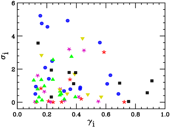
Figure 1: Results from Table 1: $ep$ (daisy); $\mu p,\mu d$ ($\circ$); $pp,pd,p\mathrm{Cu}$ ($\Box$); $\bar{p}p$ ($\nabla$); $\nu A$ ($\Delta$).

The results in Table 1 are displayed graphically in Fig. 1. This plot shows that the effective measurements are widely distributed in the $(\gamma,\sigma)$ plane. Broadly speaking, all of the experiment types contribute to all parts of the plot, with one possible exception that is explored in Sec. VI. Smaller values of $\gamma$ are more common because most aspects of the fit are constrained by more than one experiment. Smaller values of $\sigma$ are more common because the fit is reasonably self-consistent. The distribution of $\sigma$ is examined in detail in the next Section.

V Distribution of the discrepancies

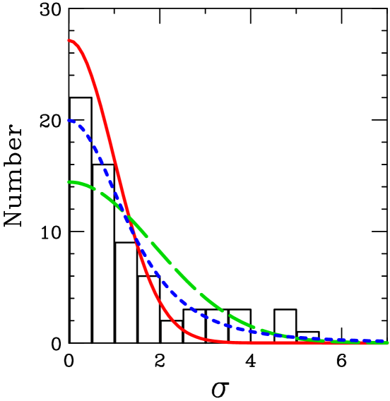
Figure 2: Distribution of the discrepancies $\sigma_{i}$ from Table 1. The solid curve is the parameter-free Gaussian prediction (10). The long-dashed curve is a fit to the scaled Gaussian form (11). The short-dashed curve is a fit to the squared-Lorentzian form (12).

According to Gaussian statistics, the 68 discrepancies $\{\sigma_{i}\}$ listed in Table 1 would be expected to follow the normal distribution

$$\frac{dP}{d\sigma}\,=\,\sqrt{\frac{1}{2\pi}}\,\exp(-\sigma^{2}/2)\;.$$ (10)

A histogram of the actual distribution is shown in Fig. 2, together with that prediction. The distribution is clearly broader than the prediction. Hence, the observed inconsistencies among the data sets are larger than what is predicted by Gaussian statistics. This can also be seen from the number of “outliers:” 10 measurements out of 68 in Table 1 have $\sigma_{i}>3\,$. The probability for so many large values to arise by random fluctuations from the distribution (10) is vanishingly small—even 5 instances of $|\sigma_{i}|>3$ in 68 tries is a million-to-one long shot.

When it is necessary to combine experimental results that lie outside a comfortable range of statistical agreement, a standard course of action is to scale up the errors—see, e.g., the Particle Data Group tables in PDG . That approach suggests fitting the histogram in Fig. 2 to a Gaussian form with adjustable width:

$$\frac{dP}{d\sigma}\,=\,\sqrt{\frac{1}{2\,\pi\,c^{2}\,}}\,\exp(-\sigma^{2}/(2\,c^{2}))\;.$$ (11)

A maximum-likelihood fit to this form yields $c=1.88\,$. This suggests that the errors in the PDF fit need to be scaled up by nearly a factor of 2 to allow for the observed inconsistencies among the data sets. This fit is also shown in Fig. 2.

Although the scaled Gaussian is an improvement over the absolute one, the fit it provides is not entirely satisfactory. A much better description of the histogram can be obtained using a form with a more slowly falling tail, such as the squared-Lorentzian:

$$\frac{dP}{d\sigma}\,=\,\frac{2\,m^{3}/\pi}{(\sigma^{2}\,+\,m^{2})^{2}}\;.$$ (12)

This curve is also shown in Fig. 2, using the parameter value $m=2.17$ obtained by maximum-likelihood fitting.

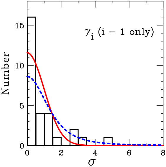
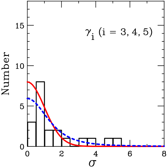
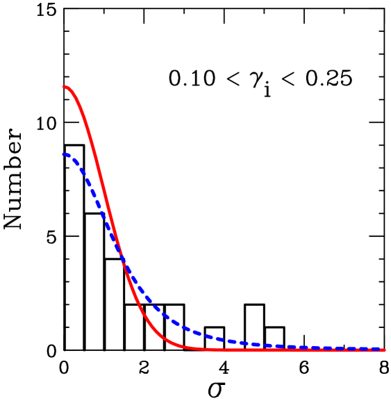
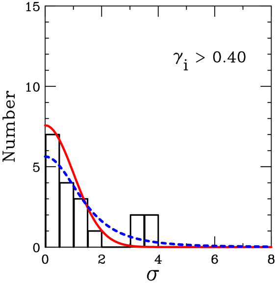
Figure 3: Distribution of the discrepancies $\sigma_{i}$ from Table 1 for measurements with: (a) $i=1$ only; (b) $i=3,4,5$; (c) $0.10<\gamma_{i}<0.25$; (d) $\gamma_{i}>0.40\,$. Curves shown are the absolute Gaussian and squared-Lorentzian curves from Fig. 2, normalized to the number of points in each histograms, but not refitted.

The distribution of discrepancies seen in Fig. 2 appears to be a general characteristic of the global fit. This is demonstrated by Fig. 3, which shows histograms for various subsets of the $(\gamma_{i},\sigma_{i})$ pairs from Table 1: (a) those with $i=1$, i.e., the best-measured parameter from each experiment; (b) those with $i=3,4,5$, i.e., less well-measured parameters from each experiment; (c) those with $0.10<\gamma_{i}<0.25$, i.e., parameters that are weakly determined by the experiment under study; and (d) those with $\gamma_{i}>0.40$, i.e., parameters that are strongly determined by the experiment under study. (The middle ranges—$\,i\!=\!2$ in (a) and (b), $0.25\!<\!\gamma_{i}\!<\!0.40$ in (c) and (d)—are excluded from these histograms in an attempt to accentuate any systematic differences.) As far as can be seen with the limited statistics, these distributions all look alike. They are all inconsistent with the absolute Gaussian prediction, and they are all consistent with the squared-Lorentzian form, whose width parameter $m=2.17$ is kept the same as in Fig. 2.

The only systematic trend that is suggested by Fig. 1 is a tendency for the muon experiments to have larger-than-average discrepancies. That trend is explored in the next Section.

VI Role of the muon experiments

Figure 1 (or Table 1) shows that the four largest discrepancies $\sigma_{i}$ all come from the $\mu p$ and $\mu d$ fixed-target BCDMS and NMC experiments. This is perhaps not surprising, since a significant tension between those experiments and the rest of the global fit was already observed in CTEQ5 CTEQ5 , using the less sophisticated method of plotting $\chi_{\mathbf{S}}^{\,2}$ vs. $\!\chi_{\mathbf{\overline{S}}}^{\,2}$ Collins . Tension between the NMC and BCDMS data sets can also be inferred from a recent MSTW paper MSTWalphas , which shows that the two experiments prefer values of $\alpha_{s}(m_{Z})$ that differ significantly, in opposite directions, from the approximate world-average value $0.118$ that is used here PDG .

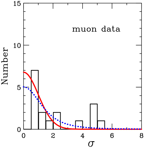
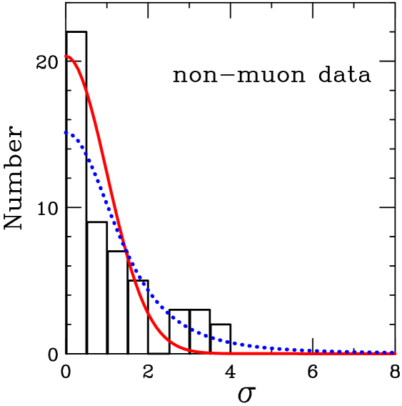
Figure 4: Distribution of the discrepancies $\sigma_{i}$ from Table 1. Left panel: $\mu p$ and $\mu d$ experiments only. Right panel: all experiments except $\mu p$ and $\mu d$. Curves are the absolute Gaussian prediction and the squared-Lorentzian fit—both the same as shown in Fig. 3 except for normalization.

Figure 4 shows the histogram of $\sigma_{i}$ for the muon experiments and the others separately. The muon histogram looks quite different: it contains zero counts in the first bin and all four of the counts with $\sigma>4$. It is therefore natural to raise the question of whether some or all of the muon experiments—or their theoretical treatment—may contain important systematic errors that have been neglected. This question is explored in detail in Sec. IX.

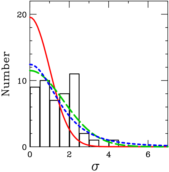
Figure 5: Distribution of the discrepancies $\sigma_{i}$ from global fits with the $\mu p$ data omitted. Solid curve is the parameter-free Gaussian prediction (10). Long dash and short dash curves are new fits to scaled-Gaussian (11) and squared-Lorentzian (12) forms respectively.

The essential question from the standpoint of this paper is whether or not the deviation from Gaussian behavior seen in Fig. 2 is a general characteristic of the PDF fits, or whether it could instead just point to problems with the muon data sets. The right hand side of Fig. 4 appears to show that the non-muon data also have a tail at large $\sigma$ which is inconsistent with the ideal Gaussian curve. However, if one speculates that the muon data or their theoretical treatment may be incorrect, then those large-$\sigma$ points might merely reflect a conflict with the muon data. A direct way to proceed is to repeat the analysis that led to Table 1, with all four of the muon experiments omitted from the global fit. In carrying this out, it was necessary to reduce the number of fitting parameters from 24 to 21 in order to obtain stable fits to the reduced input data. Results from this study are shown in Fig. 5. The distribution is again broader than the absolute Gaussian prediction, so the central conclusion from Sec. V stands even if the muon data are excluded. Because no extreme outlying points appear in this histogram, a rescaled Gaussian ($c\!=\!1.70$ in Eq. (11)) this time gives an acceptable fit. It is even slightly better than a squared-Lorentzian fit ($m=2.51$ in Eq. (12)).

The DSD method can be used to further explore the contribution of specific experiments to the global fit. This is pursued for the muon experiments in Sec. IX.

VII Non-Gaussian statistics and $\mathbf{\Delta\chi^{2}}$

This Section explains the concept of $\Delta\chi^{2}$ and estimates it for the PDF fit. Let us consider a simple scenario that is similar to the DSD situation of measuring a single variable $z_{i}$ in the symmetric case $\gamma_{i}=0.5\,$. Specifically, suppose a quantity $z$ is measured by two equally-trustworthy experiments, which report

$$\mbox{Expt 1:}\;\;z = A\,\pm\,\sqrt{2}$$

$$\mbox{Expt 2:}\;\;z = B\,\pm\,\sqrt{2}\;.$$ (13)

We wish to combine these two measurements into a single result. According to standard Gaussian statistics, that is done by taking the average and combining the errors in quadrature:

$$z=(A+B)/2\,\pm\,1\;.$$ (14)

The $\chi^{2}$ measure of fit quality is

$$\chi^{2} = \left(\frac{z-A}{\sqrt{2}}\right)^{2}\,+\,\left(\frac{z-B}{\sqrt{2}}\right)^{2}$$ (15)

$$= \left(z-\frac{A+B}{2}\right)^{2}\,+\,\left(\frac{A-B}{2}\right)^{2}\,.$$ (16)

The algebraic rearrangement in Eq. (16) reveals that the expected best-fit value $z=(A+B)/2$ indeed minimizes $\chi^{2}$, and that the error limits in (14) correspond to the points where $\chi^{2}=\chi_{\mathrm{min}}^{\,2}+\Delta\chi^{2}$ with $\Delta\chi^{2}=1$. This corresponds to the 68.3% confidence limit, i.e., “$1\,\sigma$.” The uncertainty limit for 90% confidence is farther from the minimum in $z$ by a factor $1.64$, which corresponds to $\Delta\chi^{2}=2.71\,$.

Now let us see what happens if we do not assume that the errors are Gaussian. Suppose instead that the measurements $A$ and $B$ arise from independent random processes with probability distributions

$$\frac{dP}{dA} = f(A)$$ (17)

$$\frac{dP}{dB} = f(B)\;,$$ (18)

where $\int_{-\infty}^{\infty}f(A)\,dA=1$, and we assume for simplicity that $A$ and $B$ come from the same distribution. We can assume without loss of generality that this distribution is centered about a true answer of $0$. Let us also assume that the distribution is symmetric: $f(A)=f(-A)$. It is intuitively clear that the best estimate from the two measurements will remain equal to the average $(A+B)/2$, so the real issue is how to assess the uncertainty on that result.

If the two measurements can be repeated many times, the probability distribution for their average $(A+B)/2$ is given by

$$\frac{dP}{dz} = \rho_{z}(z)$$ (19)

$$= \int_{-\infty}^{\infty}\!dA\,f(A)\int_{-\infty}^{\infty}\!dB\,f(B)\;\delta\!\left(\frac{A+B}{2}-z\right)$$

$$= 2\int_{-\infty}^{\infty}\!dA\,f(A)\,f(2z-A)\;.$$

Meanwhile, the probability distribution for the difference $(A-B)$ between the two measurements, expressed in units of its error $\sqrt{(\sqrt{2})^{2}+(\sqrt{2})^{2}}=2$, is given by

$$\frac{dP}{d\sigma} = \rho_{\sigma}(\sigma)$$ (20)

$$= \int_{-\infty}^{\infty}\!dA\,f(A)\int_{-\infty}^{\infty}\!dB\,f(B)\;\delta\!\left(\frac{A-B}{2}-\sigma\right)$$

$$= 2\int_{-\infty}^{\infty}\!dA\,f(A)\,f(A-2\sigma)\;.$$

Comparing Eqs. (19–20) and using the assumed symmetry $f(A)=f(-A)$, we obtain

$$\rho_{z}(z)\,=\,\rho_{\sigma}(z)\;.$$ (21)

Eq. (21) shows that the uncertainty distribution for the average of the two measurements is the same as the uncertainty distribution for their difference, when that difference is normalized by its error as is done here. The former is what is needed to estimate the uncertainties of the PDF results, while the latter is what is measured in the histogram of Fig. 2.

Before proceeding, let us check that the above formulae reproduce the correct results in the Gaussian case $f(A)=\exp(-A^{2}/4)/\sqrt{4\,\pi}$. In that case, Eqs. (19) and (21) give $\rho_{z}(z)=\exp(-z^{2}/2)/\sqrt{2\,\pi}$ and $\rho_{\sigma}(\sigma)=\exp(-\sigma^{2}/2)/\sqrt{2\,\pi}$. Thus $dP/dz$ and $dP/d\sigma$ are both Gaussians of width 1, which indeed agrees with the standard rules for propagating the uncertainties from Eq. (13). The middle 68.3% (90%) of the probability distribution $dP/dz$ is contained in $|z|<1.00$ ($1.64$), which corresponds to the points where $\Delta\chi^{2}=1.00$ ($2.71$), in agreement with earlier statements.

If the distribution of differences, and hence according to (21) the distribution of averages, is given by the scaled Gaussian form (11), then the uncertainty limits in $z$ are scaled by the parameter $c$ in that formula. Hence the 90% confidence tolerance becomes $\Delta\chi^{2}=2.71\,c^{2}$. For the value $c=1.88$ found in Sec. V from the fit in Fig. 2, this implies $\Delta\chi^{2}=14\,$.

If, on the other hand, the distribution of differences, and hence the distribution of averages, is given by the squared-Lorentzian form (12) with the width parameter $m=2.17$ that was found in Sec. V by fitting the distribution of differences, then the central 68.3% (90%) of the distribution is contained in $|z|<1.50$ ($2.95$), which corresponds to $\Delta\chi^{2}=2.25$ ($\Delta\chi^{2}=8.70$). Note that the ratio between 68.3% and 90% confidence points is larger for the squared-Lorentzian distribution ($8.70/2.25=3.9$) than for the Gaussian distribution ($2.71/1.00=2.7$), because of the relatively slowly-falling tail of the Lorentzian.

These results suggest that the 90% confidence criterion for the uncertainty of the global fit is given by $\Delta\chi^{2}\approx 10$.

VIII Remark on $\mathbf{\chi^{2}/N}$

The overall $\chi_{\mathrm{total}}^{\,2}$ ($=3074$) for the global fit is not far from the total number of data points ($N_{\mathrm{total}}=2970$) in the fit. This at first seems to contradict the idea that there are inconsistencies in the fit that are nearly twice the expectation based on the experimental errors. For example, in the extreme, if the actual errors for all of the data points were a factor of 2 larger than the errors claimed by the experiments, we would expect $\chi_{\mathrm{total}}^{2}/N_{\mathrm{total}}\approx 4$.

However, the actual situation does not correspond to that extreme. A given experiment with $N$ data points delivers significant information along only a few directions in parameter space—at most 5 or 6 according to Table 1. Of those directions, there is significant discord along at most 2 or 3. We can estimate the effect of this on $\chi^{2}/N$ as follows. Eq. (5) shows that the lowest possible $\chi^{2}$ for experiment $\mathbf{S}$ occurs at $\{z_{i}=A_{i}\}$, while the global best-fit value occurs at $\{z_{i}=0\}$. Hence in the global fit, $\chi_{\mathbf{S}}^{\,2}$ lies above its best-fit value by

$$\sum_{i=1}^{n}\left(\frac{A_{i}}{B_{i}}\right)^{2}\,.$$

Combining Eqs. (6–7) and using $\,\gamma_{i}A_{i}\,+\,(1-\gamma_{i})C_{i}\,=\,0$ which follows from Eq. (1), we obtain

$$A_{i}\, = \sqrt{(1-\gamma_{i})/\gamma_{i}}\;\sigma_{i}$$

$$B_{i}\, = \sqrt{1/\gamma_{i}}\;.$$ (22)

Hence the addition to $\chi^{2}$ from experiment $\mathbf{S}$ is

$$\sum_{i=1}^{n}\left(\frac{A_{i}}{B_{i}}\right)^{2}\,=\,\sum_{i=1}^{n}\,(1-\gamma_{i})\,\sigma_{i}^{\,2}.$$

Adding this up over the 68 $(\gamma_{i},\,\sigma_{i})$ pairs with $\gamma_{i}>0.1$ in Table 1 gives a total of $168\,$. The full data set has 2970 points, so this contribution of $\approx 168$ to $\chi_{\mathrm{total}}^{2}$ is not large enough to spoil the expectation that $\chi_{\mathrm{total}}^{2}\approx N_{\mathrm{total}}\pm\sqrt{2\,N_{\mathrm{total}}}$.

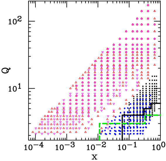
Figure 6: Kinematic region covered by the lepton DIS experiments $ep\to eX$ (H1 = $\Delta$, ZEUS = $\nabla$) and $\mu p\to\mu X$ (BCDMS=$\Box$, NMC = $\circ$).

IX Further study of the muon experiments

The largest tensions in the current PDF fit involve the four muon-initiated fixed-target experiments ($\mu p\to\mu X$ and $\mu d\to\mu X$ measured by both BCDMS and NMC), as noted in Sec. VI. The kinematic regions covered by $\mu p\to\mu X$ and $ep\to eX$ experiments are shown in Fig. 6. There is considerable overlap between the BCDMS and NMC experimental regions; but BCDMS extends farther toward $x=1\,$, while NMC extends farther toward small $x$ and small $Q$. Hence it is possible that the four muon experiments each measure different quantities. Meanwhile, the H1 and ZEUS regions overlap completely with each other, and hardly at all with the muon experiments.

Expt	N	$\chi^{2}$	$(\gamma_{1},\,\sigma_{1}),\,(\gamma_{2},\,\sigma_{2}),\,\dots$
BCDMS $F_{2}$p	339	384	$(0.88,\,2.37)$ $(0.77,\,0.31)$ $(0.57,\,\mathbf{3.03})$ $(0.44,\,\mathbf{3.54})$ $(0.12,\,\mathbf{5.79})$
BCDMS $F_{2}$d	251	248	$(0.44,\,1.98)$ $(0.31,\,0.02)$ $(0.28,\,\mathbf{3.25})$ $(0.20,\,0.07)$ $(0.18,\,0.85)$
NMC $F_{2}$p	201	332	$(0.43,\,2.16)$ $(0.26,\,0.68)$ $(0.21,\,\mathbf{5.95})$ $(0.11,\,2.94)$
NMC $F_{2}$p/d	123	121	$(0.83,\,2.73)$ $(0.78,\,1.76)$ $(0.77,\,2.04)$ $(0.62,\,1.80)$ $(0.44,\,0.36)$ $(0.26,\,0.61)$
BCDMS $F_{2}$p	339	365	$(0.89,\,1.42)$ $(0.80,\,0.71)$ $(0.78,\,0.11)$ $(0.61,\,2.95)$ $(0.41,\,0.02)$ $(0.28,\,\mathbf{3.58})$
BCDMS $F_{2}$d	251	249	$(0.46,\,2.02)$ $(0.42,\,\mathbf{3.80})$ $(0.37,\,1.49)$ $(0.29,\,0.31)$ $(0.21,\,1.24)$ $(0.17,\,0.19)$
NMC $F_{2}$p	201	331	$(0.87,\,1.74)$ $(0.57,\,2.29)$ $(0.22,\,\mathbf{4.92})$ $(0.16,\,\mathbf{4.20})$
NMC $F_{2}$p/d	123	118	$(0.89,\,\mathbf{3.65})$ $(0.80,\,2.74)$ $(0.58,\,2.52)$ $(0.48,\,0.18)$ $(0.17,\,0.31)$
BCDMS $F_{2}$p	339	365	$(0.68,\,1.50)$ $(0.64,\,0.98)$ $(0.48,\,0.11)$ $(0.35,\,2.32)$ $(0.17,\,\mathbf{3.48})$ $(0.10,\,1.37)$
BCDMS $F_{2}$d	251	260	$(0.32,\,1.55)$ $(0.28,\,0.80)$ $(0.21,\,0.81)$ $(0.18,\,\mathbf{3.47})$ $(0.15,\,1.09)$
NMC $F_{2}$p	201	338	$(0.53,\,0.37)$ $(0.21,\,\mathbf{5.48})$ $(0.15,\,\mathbf{4.54})$
NMC $F_{2}$p/d	123	119	$(0.66,\,0.88)$ $(0.55,\,\mathbf{4.05})$ $(0.45,\,0.98)$ $(0.31,\,0.53)$ $(0.15,\,0.11)$
BCDMS $F_{2}$p	250	234	$(0.69,\,0.42)$ $(0.60,\,0.99)$ $(0.46,\,0.24)$ $(0.31,\,1.11)$ $(0.12,\,2.04)\;$
BCDMS $F_{2}$d	210	188	$(0.29,\,1.64)$ $(0.26,\,2.25)$ $(0.20,\,0.91)$ $(0.18,\,2.16)$ $(0.16,\,2.79)$ $(0.12,\,2.29)$
NMC $F_{2}$p	91	135	$(0.20,\,2.01)$ $(0.11,\,1.71)$
NMC $F_{2}$p/d	71	64	$(0.59,\,2.59)$ $(0.45,\,1.87)$ $(0.32,\,0.78)$ $(0.22,\,1.11)$

Table 3: Results with $\gamma_{i}>0.1\,$ for the $\mu p$ and $\mu d$ experiments. In the first two groups, only one muon experiment—the one listed—is included in the global fit. In the last two groups, all four are included. The first group uses the same parametrizations as Table 1, while the other three groups use a parametrization with additional freedom for $u_{v}$ and $d_{v}$ at large $x$. The fourth group includes the additional kinematic cuts shown in Fig. 6.

The observed tension involving the muon experiments could arise from inconsistencies within each muon data set, or disagreements between them, or disagreements between them and the non-muon experiments. The DSD method is an excellent tool to sort this out.

The first four lines of Table 3 show results from applying the DSD method to four new global fits, in which the experiment listed is the only one of the muon experiments included in the fit. We see that large discrepancies—signaled by large $\sigma_{i}$—remain for the two $\mu p$ experiments. Those discrepancies are further indicated by elevated values of $\chi^{2}/N$: $384/339$ and $332/201$. This analysis removes the effect of any possible tension between the various muon experiments, so the discrepancies must be internal to each $\mu p$ data set, or else they reflect a conflict with the non-muon data.

Tension can also be created by insufficient flexibility in the functional forms that are used to approximate the PDFs at QCD scale $\mu_{0}$. In order to investigate this possible “parametrization dependence,” new fits were carried out in which two additional free parameters were introduced. The new parameters were added in $u_{v}(x)\equiv u(x)-\bar{u}(x)$ and $d_{v}(x)\equiv d(x)-\bar{d}(x)$, since these valence quark distributions dominate at large $x$, where the muon experiments are important according to Fig. 6. The second group of four lines in Table 3 shows the DSD results for these fits, where again only one muon experiment is included in each fit. The additional freedom produces a better agreement with the BCDMS $\mu p$ experiment, as $\chi^{2}$ drops from 384 to 365 for 339 data points. However, the $\sigma_{i}$ show that substantial tensions remain for all four of the muon experiments.

The third group of four lines in Table 3 shows results from a fit that once again includes all four muon experiments, as in Table 1; but includes the two new valence-quark parameters. One sees that this more flexible parametrization does not eliminate the tension. Further improvement cannot be obtained by further increasing the flexibility of the parametrization, because attempts to do that are foiled by the fits becoming unstable, due to large undetermined parameters.

It was possible to shed further light on the source of tension in the muon data sets by splitting each set into a low-Q and high-Q region. When this was done (not shown), it was found that both the low-Q and the high-Q portions of each muon experiment are separately consistent with the non-muon data. Hence the observed tension is generated by the Q-dependence of each muon data set.

This is actually very plausible, because the BCDMS data have previously been shown HigherTwist to contain a significant “higher-twist” component (non-leading power-law dependence in $Q$), which is not taken into account in the PDF fit. Higher-twist effects can be expected to be even more important for the NMC data, since more of that data is at small $Q$.

To suppress higher-twist contributions—or other possible deviations from NLO QCD at low $Q$—we now remove the BCDMS data that lie below the dashed line and the NMC data that lie below the solid line in Fig. 6. (These cuts were chosen roughly based on HigherTwist ; they have not been optimized.) The resulting fit, which includes all four of the muon data sets, is summarized by the final group of four lines in Table 3. With the cuts, the large tension has gone away. The $\chi^{2}/N$ for the BCDMS experiments is also greatly improved, and is now within the normal range. The $\chi^{2}/N$ is still a bit high for the NMC $\mu p$ data, which suggests that a somewhat stronger cut would be desirable for that data set.

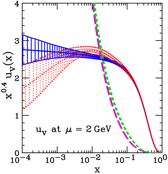
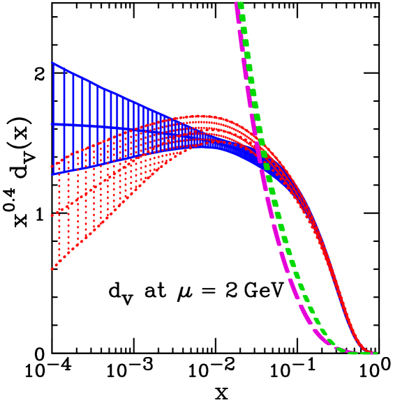
Figure 7: Uncertainty of valence quark distributions at $\Delta\chi^{2}=10$. The solid shaded region is the fit in Table 1. The dotted region is the fit in the last section of Table 3. The long-dashed and short-dashed curves show $\bar{u}$ and $\bar{d}$ respectively for comparison.

X Implications for PDF analysis

The results presented here support a tolerance criterion of $\Delta\chi^{2}\approx 10$ to estimate the 90% confidence range of PDF uncertainties, based solely on the uncertainties of the input data. In contrast, PDF determinations made using the Hessian method Hessian generally include a much broader allowed range of uncertainty, e.g. $\Delta\chi^{2}=50$ in MRST MRST2004 and $\Delta\chi^{2}=100$ for 90% confidence in CTEQ cteq66 . This larger range arises from adopting a “hypothesis-testing” criterion Collins , according to which any PDF configuration that provides a satisfactory fit to all of the input data sets is deemed acceptable. Loosely speaking, the hypothesis-testing criterion is defined by $\chi^{2}\,<\,N+\sqrt{2N}$ for each experiment. The overall allowed $\Delta\chi^{2}$ is therefore $\approx\sqrt{2N_{\mathrm{total}}}$, i.e., 77 for 3000 data points at $1\,\sigma\,$.

In detail, the hypothesis-testing condition is corrected for finite $N$ for each experiment, and refined on the basis of the lowest possible $\chi^{2}$ that can be achieved for that experiment. In the CTEQ fits cteq66 , contributions to $\chi^{2}$ from some of the data sets are enhanced by weight factors, which are chosen to keep the fits to those experiments adequate over the $\chi_{\mathrm{tot}}^{\,2}\,<\,\chi_{\mathrm{min}}^{\,2}\,+\,\Delta\chi^{2}$ range. In the most recent CTEQ fit CT09 , that procedure is supplemented by adding a quartic penalty term to the effective $\chi^{2}$, to force the fits to some recalcitrant experiments to remain satisfactory over the entire region defined by $\Delta\chi^{2}$. Meanwhile, recent MSTW fits MSTW08 ; MSTWalphas abandon the use of a fixed $\Delta\chi^{2}$, and instead determine the uncertainty limit “dynamically” along each eigenvector direction (separately for “$+$” and “$-$” senses), as the point where the fit first becomes unacceptable to one of the data sets.

The hypothesis-testing criterion is a minimal requirement for acceptable fits. It defines a broader uncertainty limit than would be predicted on normal statistical grounds, which has been called the “parameter-fitting” criterion Collins . The parameter-fitting criterion is ideally defined by $\Delta\chi^{2}=1.0$ ($2.7$) for a 68% (90%) confidence interval. In view of the results of this paper, that should be expanded in practice to $\Delta\chi^{2}\approx 10$ for 90% confidence, on the basis of inconsistencies observed among the implications of different data sets.

From a statistical point of view, the hypothesis-testing criterion appears to be overly conservative. That notion is challenged, however, by the apparent “time-dependence” and “space-dependence” of the PDFs. Namely, we have repeatedly seen changes from one generation of PDFs to the next, e.g., CTEQ5/CTEQ6.0/CTEQ6.1/CTEQ6.6/CT09 or MRST2001/MRST2002/MRST2004/MSTW2008, for which the central estimate for some flavor in a set is close to the predicted 90% confidence limit from the previous set; and differences between PDF sets determined by different groups, such as CTEQ and MSTW, are also frequently as large as these broad uncertainty estimates. Examples of this can be seen in Figs. 8 and 12 of CT09 .

Some of the time-dependence has resulted from improvements in the theory, such as the better treatment of heavy quark mass effects beginning with CTEQ6.6; or additions to the available data. But other differences between PDF determinations arise from the choices of which data sets to include; in choices of kinematic cuts such as those introduced in Sec. IX to remove data points for which the perturbative QCD treatment is suspect; and in the choice of parametrizing functions at $\mu_{0}$. Additional uncertainties are present due to the NLO approximations made in the theory. Adopting the hypothesis-testing criterion can be seen as an expedient way to broaden the estimated uncertainty range to allow for these uncertainties—although obviously they cannot be reliably predicted on the basis of the errors in the experimental data sets.

Quantities that are weakly constrained by the data are especially subject to parametrization dependence. A classic example of this is provided by the gluon distribution at large $x$. Prior to measurements of the inclusive jet cross section at the Tevatron, there was very little information on the gluon at large $x$. The parametrizations used at that time therefore devoted very few parameters to the large-$x$ region, since unconstrained parameters make the fitting procedure unstable. When the jet data became available, they were found to lie outside the predicted uncertainty range. This pointed to a need to introduce additional parameters, which could then be determined by stable fits using the new data.

A further example is shown in Fig. 7, which displays the valence quark distributions $u_{v}\equiv u-\bar{u}$ and $d_{v}\equiv d-\bar{d}$. Their uncertainty is large for $x\,\lesssim\,0.01$, because their contribution from that region to most observables is swamped by much larger contributions from $\bar{u}$ and $\bar{d}$, which are also shown in the figure. The uncertainties are shown for both the original fit (described in Table 1) and the final fit (described in the last four lines of Table 3). The final central fit lies far outside the uncertainty band estimated in the earlier fit, when that uncertainty is computed at $\Delta\chi^{2}=10$. At large $x$, the situation is reversed: valence quarks dominate the phenomenology, so $u_{v}$ and $d_{v}$ are very well measured there, and the difference between the two fits is small and consistent with the estimated uncertainty.

An emerging alternative to the Hessian approach is provided by the NNPDF NNPDF method, which avoids the parametrization problem by using very flexible Neural Network representations instead of functional forms to describe the PDFs at $\mu_{0}$. An attractive feature of the NNPDF approach is that introducing new measurements reduces the uncertainty of the output PDFs, unless the new data are rather inconsistent with the previous data. The same cannot be said for the Hessian approach, because when new data sets are added to the global fit, it is often desirable to increase the flexibility of the parametrization, as happened with the inclusive jet cross section as discussed above. The NNPDF method incorporates experimental errors by creating an ensemble of fits to “pseudodata” sets in which the measured values are displaced by random shifts that are proportional to the experimental uncertainties. It would be interesting to apply the NNPDF method to assess the uncertainties that are not associated with the experimental errors, by using the original unshifted data to produce each element in the ensemble. The ensemble would then retain the other sources of uncertainty due to the other random processes used to create it.

The effective number of parton parameters that can be measured by the available data—currently around 25—is small enough that the traditional Hessian method is convenient. But the number of potential parameters that could be determined by some future experiment, but which are currently unconstrained, is of course very large or even infinite. So it is not practical to provide parameters for all such potential degrees of freedom. However, the Hessian approach may nevertheless be viable for the large range of predictions for which PDFs are needed, since the processes one wishes to predict depend on similar aspects of the PDFs to the experiments that are used to determine them. As an extreme case in point, the PDF fits described in this paper admit no uncertainty at all in the assumption $s(x,\mu)=\bar{s}(x,\mu)$. They can therefore not be used to predict new processes that are sensitive to the strangeness asymmetry $s^{(-)}(x,\mu)\equiv s(x,\mu)-\bar{s}(x,\mu)$; but most processes we wish to predict are not in fact sensitive to that asymmetry.

XI Conclusion

The recently-developed DSD method DSD has been applied to assess compatibility among the data sets that are used to extract parton distribution functions. The DSD method is more discerning than the previous method Collins ; CT09 of studying correlations between $\chi^{2}$ values for the various experiments, because it looks for inconsistencies of each experiment along the specific directions in parameter space for which that experiment is significant in the global fit, while ignoring the large number of directions along which the experiment is unimportant.

Results from the DSD method, which are shown in Table 1, can be read as a “report card” on the contribution of each experiment to the global fit. The $\gamma_{i}$ parameters measure how much each experiment influences the fit, while the $\sigma_{i}\,$ parameters measure how much dissonance each experiment brings with it.

Table 1 identified fixed-target $\mu p$ and $\mu d$ experiments as the greatest source of tension in a recent global fit. Further exploration in Sec. IX revealed the underlying cause of that tension as deviations from NLO QCD predictions—presumably due to higher twist—which had previously been observed in these data HigherTwist , but which were not taken into account in the fit. Kinematic cuts shown in Fig. 6 remove the contaminated region and eliminate the large discrepancies, as can be seen by comparing the last four lines of Table 3 with their corresponding entries in Table 1. Future global fits should make a refined version of these cuts, or else introduce additional fitting parameters to model the higher-twist contribution. (The latter was attempted in CTEQ6 cteq60 , without conclusive results—the DSD method not being available at that time to make a sensitive test of the consistency.)

Independently of the muon experiments, the implications of the various data sets in the global fit are found to be somewhat inconsistent with each other (Fig. 5). The average discrepancy is a bit less than a factor of 2 larger than what is predicted by straightforward propagation of the experimental errors. This was shown in Sec. VII to suggest that the 90% confidence limit for predictions from the global fit should be estimated by a tolerance criterion of $\Delta\chi^{2}\approx 10$, in place of the $\Delta\chi^{2}=2.71$ that would be implied by pure Gaussian statistics.

Much larger tolerance criteria ($\Delta\chi^{2}=50$ MRST2004 or $\Delta\chi^{2}=100$ cteq60 ; cteq66 ) have been used to estimate the 90% confidence limit in recent applications of the Hessian approach. These more conservative tolerance criteria correspond to the “hypothesis testing” notion that any PDF set is acceptable as long as its fit to every data set lies in the nominal statistical range $\chi^{2}=N\,\pm\,\sqrt{2N}$, or its 90% analog, with appropriate corrections for finite $N$. This implies an effective overall $\Delta\chi_{\mathrm{total}}^{2}\sim\sqrt{2N_{\mathrm{total}}}\approx 75$ for $1\,\sigma$. The uncertainty from input data, as assessed in this paper by studying its mutual consistency, does not call for this expanded uncertainty range. However, some aspects of the fit do no doubt require an expanded uncertainty estimate, because of theoretical systematic errors—most notably the use of NLO perturbation theory and parametrization dependence. The need for some such expanded uncertainty is demonstrated by the relatively large changes in uncertainty bands that can be caused by relatively minor changes in the choice of parametrization or in the choice of data sets that are included. Examples of this are provided by the valence quark distributions at small $x$, as discussed in Sec. IX; and the gluon distribution, as discussed in CT09 .

In the future, it would be desirable to estimate the uncertainties associated with parametrization choices and other theoretical errors directly, rather than using a large $\Delta\chi^{2}$ to stand in for them in a manner that is based artificially on the uncertainties of the data. If this can be accomplished, the result will likely expand the estimated uncertainty range for quantities that are poorly constrained; but it may reduce the uncertainty for quantities that are well constrained, because of the reduction in $\Delta\chi^{2}$. From the ratio of $\Delta\chi^{2}$ values, one might hope to find the uncertainty reduced by as much as a factor of 3; but the actual reduction will probably be less than that, because $\chi^{2}$ generally rises faster than quadratic for large displacements from the best fit.

Appendix

A formal derivation of the DSD method was presented in DSD , and it is reviewed in Sec. III. To assist in understanding the method, this Appendix illustrates it by a simple explicit example.

Suppose we have a theory that predicts a linear relationship $y=ax+b$ where $a$ and $b$ are unknown parameters. Further suppose there are three experiments, which have measured

$$\mbox{Expt 1:}\;\;y = y_{1}\,\pm 1\;\mbox{ at }x=-1$$

$$\mbox{Expt 2:}\;\;y = y_{2}\,\pm 1\;\mbox{ at }x=\;\;0$$

$$\mbox{Expt 3:}\;\;y = y_{3}\,\pm 1\;\mbox{ at }x=\;\;1\;.$$ (23)

The fit to these three experiments is described by

$$\chi^{2}=\chi_{1}^{\,2}\,+\,\chi_{2}^{\,2}\,+\,\chi_{3}^{\,2}\;,$$ (24)

where

$$\chi_{1}^{\,2} = \left(\frac{y_{1}\,-\,(-a+b)}{1}\right)^{2}$$

$$\chi_{2}^{\,2} = \left(\frac{y_{2}\,-\,(b)}{1}\right)^{2}$$

$$\chi_{3}^{\,2} = \left(\frac{y_{3}\,-\,(a+b)}{1}\right)^{2}\;.$$ (25)

It is natural to replace the theory parameters $a$ and $b$ by new parameters $u_{1}$ and $u_{2}$ that are measured from the minimum point in $\chi^{2}$ and normalized in the standard Hessian way:

$$a = \frac{u_{1}}{\sqrt{2}}\,+\,\frac{y_{3}-y_{1}}{2}$$

$$b = \frac{u_{2}}{\sqrt{3}}\,+\,\frac{y_{1}+y_{2}+y_{3}}{3}\;.$$ (26)

This puts $\chi^{2}$ into the standard diagonal form

$$\chi^{2}\,=\,u_{1}^{\,2}\,+\,u_{2}^{\,2}\,+\,K^{2}\;,$$ (27)

where

$$K\,=\,(y_{1}+y_{3}-2y_{2})/\sqrt{6}\;.$$ (28)

The transformation (26) that yields (27) contains a shift and a rescaling of the original fitting parameters $a$ and $b$. In general, it also requires a rotation (orthogonal transformation) that intermingles those variables; but that was not necessary in this simple example because of symmetry. The uncertainty on the theory parameters $a$ and $b$ in the global fit can now be obtained easily from Eq. (27), which implies that the $1\,\sigma$ limits are $u_{1}=0\pm 1$ and $u_{2}=0\pm 1$.

In order to examine the internal consistency of this fit, we must consider the contributions to $\chi^{2}$ from the individual experiments. These can be expressed in terms of the new coordinates as

$$\chi_{1}^{\,2} = \left(\frac{u_{1}}{\sqrt{2}}\,-\,\frac{u_{2}}{\sqrt{3}}\,+\,\frac{K}{\sqrt{6}}\right)^{2}$$

$$\chi_{2}^{\,2} = \left(\frac{u_{2}}{\sqrt{3}}\,+\,\frac{2K}{\sqrt{6}}\right)^{2}$$

$$\chi_{3}^{\,2} = \left(\frac{u_{1}}{\sqrt{2}}\,+\,\frac{u_{2}}{\sqrt{3}}\,-\,\frac{K}{\sqrt{6}}\right)^{2}\;.$$ (29)

To study the consistency between Expt 1 and its complement, it is necessary to make a further coordinate transformation to diagonalize $\chi_{1}^{\,2}\,$. That transformation can be found by the DSD method; or in this simple case, by inspection:

$$u_{1} = \quad\sqrt{3/5}\,v_{1}\,+\,\sqrt{2/5}\,v_{2}$$

$$u_{2} = -\,\sqrt{2/5}\,v_{1}\,+\,\sqrt{3/5}\,v_{2}\;.$$ (30)

This gives

$$\chi_{1}^{\,2} = \left(\frac{v_{1}\,+\,\sqrt{1/5}\,K}{\sqrt{6/5}}\right)^{2}$$

$$\chi_{\overline{1}}^{\,2}\,=\,\chi_{2}^{\,2}\,+\,\chi_{3}^{\,2} = \left(\frac{v_{1}\,-\,\sqrt{5}\,K}{\sqrt{6}}\right)^{2}\,+\,v_{2}^{\,2}$$

$$\chi^{2}=\chi_{1}^{\,2}\,+\,\chi_{\overline{1}}^{\,2} = v_{1}^{\,2}\,+\,v_{2}^{\,2}\,+K^{2}\;.$$ (31)

From this, one easily reads

$$\mbox{Expt 1:}\quad v_{1} = -\,\sqrt{1/5}\,K\,\pm\,\sqrt{6/5}$$

$$\mbox{Expt $\overline{\mbox{1}}$:}\quad v_{1} = +\,\sqrt{5}\,K\,\pm\,\sqrt{6}\;.$$ (32)

Subtracting these two measurements and combining their errors in quadrature shows that they differ by $\sqrt{36/5}\,K\,\pm\,\sqrt{36/5}$. This differs from $0$ by $K\,$ standard deviations, which is the measure of consistency between Expt 1 and its complement.

The contribution to $\chi^{2}$ from Expt 2 in Eq. (29) happens to be already in the diagonal form that is the heart of the DSD method, so it requires no further transformation:

$$\chi_{2}^{\,2} = \left(\frac{u_{2}\,+\,\sqrt{2}K}{\sqrt{3}}\right)^{2}$$

$$\chi_{\overline{2}}^{\,2}\,=\,\chi_{1}^{\,2}\,+\,\chi_{3}^{\,2} = u_{1}^{\,2}\,+\,\left(\frac{u_{2}\,-\,\sqrt{1/2}\,K}{\sqrt{3/2}}\right)^{2}\;.$$ (33)

From this, one reads

$$\mbox{Expt 2:}\quad u_{2} = -\,\sqrt{2}\,K\,\pm\,\sqrt{3}$$

$$\mbox{Expt $\overline{\mbox{2}}$:}\quad u_{2} = +\,\sqrt{1/2}\,K\,\pm\,\sqrt{3/2}\;.$$ (34)

Subtracting these results and combining their errors in quadrature shows that the measurement of $u_{2}$ by Expt 2 and its complement differ by $\sqrt{9/2}\,K\,\pm\,\sqrt{9/2}$. This difference is also $K$ standard deviations away from $0\,$.

Because there are only three data points in this example, with two free parameters in the theory, there is only one possible test of the internal consistency. That is why both Expt 1 and Expt 2 show the same discrepancy $K$, when the discrepancy is measured in standard deviations. To show that Expt 3 would also give the same result is left as an exercise for the reader!

In this simple example, the consistency measure can also be found by elementary means: adding the errors from (23) in quadrature gives $\pm\,\sqrt{6}$ for the uncertainty of $y_{1}+y_{3}-2y_{2}$, and hence the uncertainty of $K$ is $\pm 1$ by Eq. (28). Meanwhile, the theoretical prediction for $K$ is $0$, since the theory predicts $y$ to be a linear function of $x$, and $y_{1}$, $y_{2}$, $y_{3}$ are measured symmetrically at $x=-1,0,1$. Hence the difference between theory and experiment is $K\pm 1$, so $K$ is indeed the discrepancy measured in standard deviations.

References

- (1) J. Pumplin, D. R. Stump, J. Huston, H. L. Lai, P. M. Nadolsky and W. K. Tung, JHEP 0207, 012 (2002) [arXiv:hep-ph/0201195].
- (2) P. M. Nadolsky et al., Phys. Rev. D 78, 013004 (2008) [arXiv:0802.0007 [hep-ph]].
- (3) J. Pumplin, J. Huston, H. L. Lai, W. K. Tung and C. P. Yuan, Phys. Rev. D 80, 014019 (2009) [arXiv:0904.2424 [hep-ph]].
- (4) A. D. Martin, W. J. Stirling, R. S. Thorne and G. Watt, arXiv:0901.0002 [hep-ph].
- (5) R. D. Ball et al. [NNPDF Collaboration], Nucl. Phys. B 809, 1 (2009) [arXiv:0808.1231 [hep-ph]]; A. Guffanti, J. Rojo and M. Ubiali, “The NNPDF1.2 parton set: implications for the LHC,” arXiv:0907.4614 [hep-ph].
- (6) J. Pumplin, Phys. Rev. D 80, 034002 (2009) [arXiv:0904.2425 [hep-ph]].
- (7) J. Pumplin, D. R. Stump and W. K. Tung, Phys. Rev. D 65, 014011 (2001) [arXiv:hep-ph/0008191]; J. Pumplin et al., Phys. Rev. D 65, 014013 (2001) [arXiv:hep-ph/0101032].
- (8) T. Aaltonen et al. [CDF Collaboration], Phys. Rev. D 78, 052006 (2008) [arXiv:0807.2204 [hep-ex]].
- (9) V. M. Abazov et al. [D0 Collaboration], Phys. Rev. Lett. 101, 062001 (2008) [arXiv:0802.2400 [hep-ex]].
- (10) C. Adloff et al. [H1 Collaboration], Eur. Phys. J. C 21, 33 (2001) [arXiv:hep-ex/0012053].
- (11) C. Adloff et al. [H1 Collaboration], Eur. Phys. J. C 19, 269 (2001) [arXiv:hep-ex/0012052].
- (12) C. Adloff et al. [H1 Collaboration], Eur. Phys. J. C 30, 1 (2003) [arXiv:hep-ex/0304003].
- (13) C. Adloff et al. [H1 Collaboration], Eur. Phys. J. C 13, 609 (2000) [arXiv:hep-ex/9908059].
- (14) S. Chekanov et al. [ZEUS Collaboration], Eur. Phys. J. C 21, 443 (2001) [arXiv:hep-ex/0105090].
- (15) S. Chekanov et al. [ZEUS Collaboration], Phys. Rev. D 70, 052001 (2004) [arXiv:hep-ex/0401003].
- (16) J. Breitweg et al. [ZEUS Collaboration], Eur. Phys. J. C 12, 411 (2000) [Erratum-ibid. C 27, 305 (2003)] [arXiv:hep-ex/9907010].
- (17) S. Chekanov et al. [ZEUS Collaboration], Eur. Phys. J. C 32, 1 (2003) [arXiv:hep-ex/0307043].
- (18) S. Chekanov et al. [ZEUS Collaboration], Phys. Lett. B 539, 197 (2002) [Erratum-ibid. B 552, 308 (2003)] [arXiv:hep-ex/0205091].
- (19) A. C. Benvenuti et al. [BCDMS Collaboration], Phys. Lett. B 223, 485 (1989).
- (20) A. C. Benvenuti et al. [BCDMS Collaboration], Phys. Lett. B 237 (1990) 592.
- (21) M. Arneodo et al. [New Muon Collaboration], Nucl. Phys. B 483, 3 (1997) [arXiv:hep-ph/9610231].
- (22) G. Moreno et al., Phys. Rev. D 43, 2815 (1991).
- (23) R. S. Towell et al. [FNAL E866/NuSea Collaboration], Phys. Rev. D 64, 052002 (2001) [arXiv:hep-ex/0103030].
- (24) J. C. Webb et al. [NuSea Collaboration], arXiv:hep-ex/0302019.
- (25) F. Abe et al. [CDF Collaboration], Phys. Rev. Lett. 74, 850 (1995) [arXiv:hep-ex/9501008].
- (26) D. E. Acosta et al. [CDF Collaboration], Phys. Rev. D 71, 051104 (2005) [arXiv:hep-ex/0501023].
- (27) U. K. Yang et al. [CCFR/NuTeV Collaboration], Phys. Rev. Lett. 86, 2742 (2001) [arXiv:hep-ex/0009041].
- (28) W. G. Seligman et al., Phys. Rev. Lett. 79, 1213 (1997) [arXiv:hep-ex/9701017].
- (29) J. P. Berge et al., Z. Phys. C 49, 187 (1991).
- (30) M. Goncharov et al. [NuTeV Collaboration], Phys. Rev. D 64, 112006 (2001) [arXiv:hep-ex/0102049].
- (31) C. Adloff et al. [H1 Collaboration], Phys. Lett. B 528, 199 (2002) [arXiv:hep-ex/0108039].
- (32) A. Aktas et al. [H1 Collaboration], Eur. Phys. J. C 45, 23 (2006) [arXiv:hep-ex/0507081].
- (33) A. Aktas et al. [H1 Collaboration], Eur. Phys. J. C 40, 349 (2005) [arXiv:hep-ex/0411046].
- (34) S. Chekanov et al. [ZEUS Collaboration], Eur. Phys. J. C 28, 175 (2003) [arXiv:hep-ex/0208040].
- (35) J. Breitweg et al. [ZEUS Collaboration], Eur. Phys. J. C 12, 35 (2000) [arXiv:hep-ex/9908012].
- (36) S. Chekanov et al. [ZEUS Collaboration], Phys. Rev. D 69, 012004 (2004) [arXiv:hep-ex/0308068].
- (37) C. Amsler et al. [Particle Data Group], Phys. Lett. B 667, 1 (2008).
- (38) H. L. Lai et al. [CTEQ Collaboration], Eur. Phys. J. C 12, 375 (2000) [arXiv:hep-ph/9903282].
- (39) J. C. Collins and J. Pumplin, “Tests of goodness of fit to multiple data sets,” arXiv:hep-ph/0105207.
- (40) A. D. Martin, W. J. Stirling, R. S. Thorne and G. Watt, arXiv:0905.3531 [hep-ph].
- (41) M. Virchaux and A. Milsztajn, Phys. Lett. B 274, 221 (1992).
- (42) A. D. Martin, R. G. Roberts, W. J. Stirling and R. S. Thorne, Phys. Lett. B 604, 61 (2004) [arXiv:hep-ph/0410230].