Fracturing the optimal paths

Abstract

Optimal paths play a fundamental role in numerous physical applications ranging from random polymers to brittle fracture, from the flow through porous media to information propagation. Here for the first time we explore the path that is activated once this optimal path fails and what happens when this new path also fails and so on, until the system is completely disconnected. In fact numerous applications can be found for this novel fracture problem. In the limit of strong disorder, our results show that all the cracks are located on a single self-similar connected line of fractal dimension $D_{b}\approx 1.22$. For weak disorder, the number of cracks spreads all over the entire network before global connectivity is lost. Strikingly, the disconnecting path (backbone) is, however, completely independent on the disorder.

The identification and characterization of the optimal path in a disordered landscape represents an important problem in theoretical and computational physics as it can be intimately associated with many relevant scientific and technological applications Mezard84 ; Ansari85 ; Huse85 ; Kirkpatrick85 ; Kardar86 ; Kertesz92 ; Perlsman92 ; Havlin05 including brittle fracture, random polymers and transport in porous media. It has been shown that optimal paths extracted from energy landscapes generated with weak disorder are self-affine and belong to the same universality class of directed polymers Schwartz98 . In the strong disorder or ultrametric limit, on the other hand, numerical works Cieplak94 ; Porto97 ; Porto99 demonstrated the self-similar nature of the optimal path on two and three-dimensional lattices with fractal dimensions given by $D_{f}\approx 1.22$ and $1.43$, respectively.

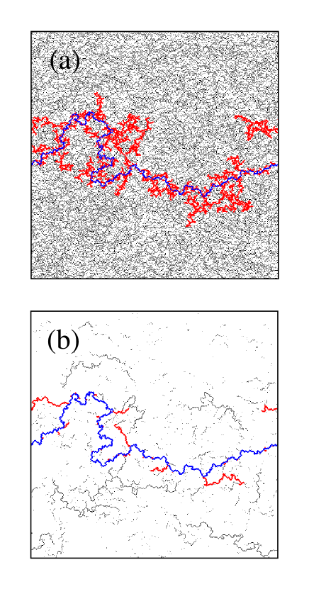
Figure 1: (Color online) Typical realizations of the OPC model on a $512\times 512$ lattice. In (a) the blocked sites generated under weak disorder conditions ($\beta=0.002$) can be categorized in three distinct types, namely, the loopless backbone of the OPC (shown in blue) at which multiple dangling ends (shown in red) are attached, and isolated clusters (shown in black) spread all over the network. As shown in (b), under moderate disorder conditions ($\beta=6.0$), while the OPC backbone is preserved, the number of dangling ends and isolated clusters is substantially reduced. Under conditions of very strong disorder (not shown), only the OPC backbone remains.

Optimal paths can be chosen by nature as those of minimum energy as occurs for instance in electrical or fluid flow through random media or they can be chosen deliberately in man made devices to reduce a cost function as for instance in internet or car traffic. Since these paths are heavily used they are more likely prone to failure either by overload, overheating or congestion. Two questions that naturally arise are (i) how and when the system will eventually collapse and (ii) how the topology and inhomogeneity of this fracture affects its performance. It is the aim of the present Letter to provide a novel modelization for this complex problem that captures its essential features and gives some insight about the statistical physics of these important questions. We first introduce a new model to generate a macroscopic fault line, namely the Optimal Path Crack (OPC) method, that is based on an iterative application of the Dijkstra algorithm Dijkstra59 to two-dimensional random landscapes. We then quantify the effect of disorder on the resulting crack topology to substantiate the relevance of the OPC method as a tool to understand the fracture of the random medium.

Our substrate is a square lattice of size $L$ with fixed boundary conditions at the top and bottom, and periodic boundary conditions in the transversal direction. Disorder is introduced in our model by assigning to each site $i$ an energy value $\epsilon_{i}=\exp[\beta(p_{i}-1)]$ Braunstein02 , where $p_{i}$ is a random variable uniformly distributed in the interval $[0,1]$, and $\beta$ is a positive parameter that has the physical meaning of inverse temperature. It can be readily shown that this transformation is equivalent to choosing the values of $\epsilon$ from a power-law distribution, namely $P(\epsilon_{i})\sim{1/\epsilon_{i}}$, subjected to a maximum cutoff given by $\epsilon_{max}=e^{\beta}$. The existence of such a cutoff turns the hyperbolic distribution normalizable for any finite value of $\beta$. In this way, $\beta$ represents the strength of disorder since it controls the broadness of the energy distribution.

The energy of any path in the system is defined here as the sum of all the energies of its sites. In particular, the optimal path is the one among all paths connecting the bottom to the top of the lattice that has the smallest sum over all energies of its sites. This definition is similar, but different from the definition of the shortest path in a network Stauffer94 . Without loss of generality, since we only consider positive $p_{i}$ values, the Dijkstra algorithm becomes a suitable tool for finding the optimal path Dijkstra59 .

The OPC is formed as follows. Once the first optimal path connecting the bottom and the top of the lattice is determined, we search for its site having the highest energy which then becomes the first blocked site, i.e., that can no longer be part of any path. This is equivalent to impose an infinite energy to this site. Next, the optimal path is calculated among the remaining accessible sites of the lattice, from which the highest energy site is again removed, and so on. The blocked sites can be viewed as “micro-cracks”, and the process continues iteratively until the system is disrupted and we can no longer find any path connecting bottom to top.

In Fig. 1a we show the resulting spatial distribution of blocked sites that constitutes the OPC in a typical random landscape generated under weak disorder conditions ($\beta=0.002$). As depicted, the OPC structure has three basic elements. Besides the loopless backbone of the fracture (shown in blue) which effectively “breaks” the system in two, we can observe the presence of dangling ends (shown in red) as well as isolated clusters homogeneously distributed over the entire network (shown in black). The situation becomes very different when we increase the value of the disorder parameter $\beta$. As shown in Fig. 1b, the amount of dangling ends and isolated clusters in a OPC generated under moderate disorder conditions ($\beta=6.0$) becomes significantly smaller than in the case of weak disorder. By increasing further the value of $\beta$, finally only the backbone remains. Interestingly this backbone is identical for all values of $\beta$, while the entire set of blocked sites is highly dependent on the way disorder is introduced in the system.

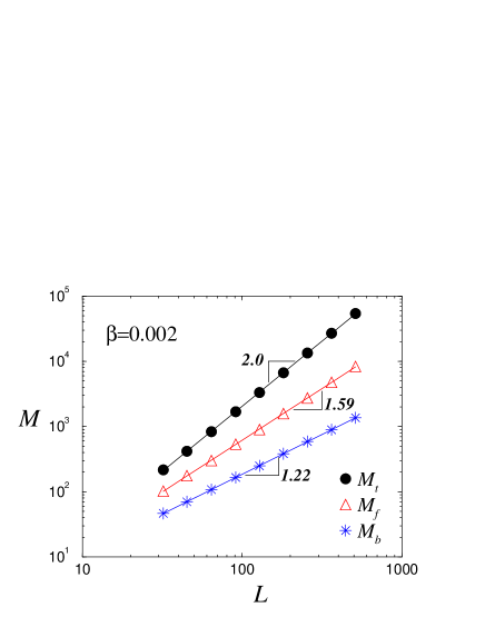
Figure 2: (Color online) Logarithmic dependence on size of the mass of all blocked sites $M_{t}$ (circles) forming the OPC, the cluster of all sites in the fracture $M_{f}$ (triangles), and the backbone mass $M_{b}$ of the OPC that divides the system in two (stars), for $\beta=0.002$. The system is considered to be in the weak disorder regime for this value of $\beta$ and this range of system sizes. The three solid lines are the least-squares fits to the data of power-laws, $M_{t}\simeq L^{D_{t}}$, $M_{f}\simeq L^{D_{f}}$ and $M_{b}\simeq L^{D_{b}}$, with exponents $D_{t}=2.00\pm 0.01$, $D_{f}=1.59\pm 0.02$, and $D_{b}=1.22\pm 0.02$, respectively.

The behavior shown in Fig. 1 is somehow related to the problem of minimum path in disordered landscapes Porto99 . In that case, the passage from weak to strong disorder in the energy distribution reveals a sharp crossover between self-affine and self-similar behaviors of the optimal path. In the strong disorder regime the energy of the minimum path is controlled by the energy of a single site. This situation occurs when the distribution of energies can not be normalized, for instance, in the case of a power-law distribution, $P(\epsilon_{i})\sim{\epsilon_{i}^{-\alpha}}$, for $\alpha\leq{1}$. The parameter $\beta$ alone, however, does not determine the limit between weak and strong disorder, since this property also depends significantly on the system size. More precisely, if $\beta$ is sufficiently high, or the lattice size is sufficiently small, the sampling of the distribution near the cutoff region is not so relevant. For any practical purpose, this network is considered to be in the strong disorder regime, resulting in a self-similar type of scaling for the minimum path. By increasing the network size, we may reach the point where one should expect to start sampling larger energy values that are beyond the cutoff of the distribution. Above this scale, the system will return to the weak disorder regime, leading to a self-affine behavior for the minimum path. In this way we should expect an abrupt transition from the weak disorder regime, at small values of $\beta$, to the strong disorder regime, at large values of $\beta$ Porto99 .

In order to quantify macroscopically the effect of disorder on the geometry of the OPC, we performed computer simulations for $1000$ realizations of lattices with sizes varying in the range $32\leq L\leq 512$, and generated with different values of the disorder parameter $\beta$. In Fig. 2 we show for $\beta=0.002$ that the average mass of the OPC backbone scales as $M_{b}\simeq L^{D_{b}}$, with an exponent $D_{b}=1.22\pm 0.02$ self-affine . Surprisingly, this exponent value is statistically identical to the fractal dimension previously found for the optimal path line, but obtained under strong disorder Cieplak94 ; Porto97 ; Porto99 . It is also very close to that found “strands” in Invasion Percolation ($1.22\pm 0.01$ Cieplak94 ), and paths on Minimum Spanning Trees ($1.22\pm 0.01$ Dobrin01 ). In our case, however, it is important to note that the value of $D_{b}$ reflects a highly non-local property of the system that is intrinsically associated with the iterative process involved in the OPC calculation. Also shown in Fig. 2 is the mass of the OPC fracture in weak disorder, which consists of both the backbone and its dangling ends. While the crack itself grows as a power-law with size, $M_{f}\simeq L^{D_{f}}$, with an exponent $D_{f}=1.59\pm 0.02$, the total mass of blocked sites (crack and isolated clusters), however, is a constant fraction of the total mass of the system, i.e. $M_{t}\simeq L^{2}$.

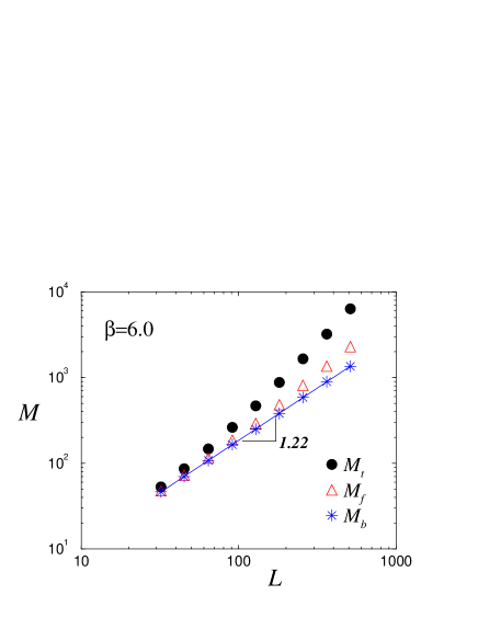
Figure 3: (Color online) Log-log plot of the masses $M_{t}$ (circles), $M_{f}$ (triangles) and $M_{b}$ (stars) against system size $L$ for $\beta=6.0$. For this intermediate value of $\beta$, we can clearly identify the crossover from strong to weak disorder depending on the system scale. For small lattices, the system operates under strong disorder conditions. As a consequence, most of the blocked sites lie on the fracture path and the three masses $M_{t}$, $M_{f}$ and $M_{b}$ are identical. As the system size increases, one reaches the weak disorder regime, and the three curves split apart. At larger scales, we should recover the same power-law behaviours found for sufficiently low values of $\beta$, as shown in Fig. 2.

In Fig. 3, the results obtained for $\beta=6.0$ clearly indicate the transition from strong to weak disorder regimes by systematically increasing the size of the system. As already mentioned, the stronger the disorder in the system (low $L$ or high $\beta$), the smaller is the number of final blocked sites that also become more and more localized in a singly-connected crack line. Precisely, in the limit of very strong disorder, we obtain that only the OPC backbone mass $M_{b}$ remains, i.e. $M_{t}\rightarrow M_{b}$ and $M_{f}\rightarrow M_{b}$, scaling in the same way as in the weak disorder limit, namely $M_{b}\simeq L^{D_{b}}$, with $D_{b}=1.22\pm 0.02$. As shown in Fig. 1, the backbone is indeed invariant under the change of $\beta$. By increasing the value of $L$, we observe a gradual departure of $M_{t}$ and $M_{f}$ from this behavior to their respective scaling laws in weak disorder (high $L$ or low $\beta$), as displayed in Fig. 2.

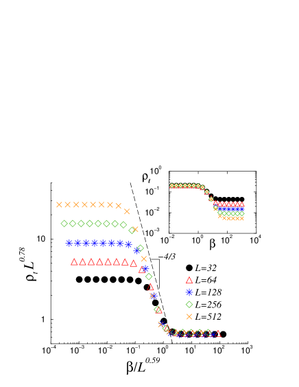
Figure 4: (Color online) Transition from weak to strong disorder in the OPC model. In these curves we plot the density of all blocked sites $\rho_{t}$ at the end of the process when the top of the system disconnects from the bottom. These curves present three distinct regimes. For weak disorder $\beta<1$ one sees a saturation in the density in a value around $\rho_{t}\approx{0.22}$. For intermediate values one sees the density decreasing with the disorder parameter $\beta$, however there is no dependence on the system size. For larger values of $\beta$ we see the density saturating again, but now to a value that depends on the system size $L$. This last regime is the one that characterizes the strong disorder regime. The saturated density in this regime depends on the system size as $L^{D_{b}-2}$, where $D_{b}\approx{1.22}$ is the fractal dimension of the OPC backbone. For each system size, we observe the transition to the strong disorder regime at a different value of the parameter $\beta_{\times}$. From the collapse shown in the inset, a non-trivial dependence is revealed between the onset of the transition and the system size, $\beta_{\times}\sim{L^{0.59}}$.

The transition from weak to strong disorder is better illustrated by the results depicted in the inset of Fig. 4. There we plot the density of all blocked sites $\rho_{t}$ at the end of the process as a function of the parameter $\beta$. The curves exhibit three different regimes, depending on the value of $\beta$. For small values, $\beta<1$, the density saturates to a fixed value. For larger values, the density decays as a power-law $\rho_{t}\sim\beta^{-\theta}$, with an exponent $\theta\approx 4/3$. Both regimes, saturation and power-law decay, are still in weak disorder. For finite lattices, the curves present another crossover to a minimum density that is now dependent on the system size. This second crossover, $\beta_{\times}$, which indicates the transition to strong disorder, should depend on the system size in such way that an infinite system is in weak disorder for any finite value of $\beta$. For large enough values of $\beta$, in the strong disorder regime, the density reaches a minimum value when all the blocked sites lie on the fracture dividing the system. As shown in Fig. 2, the mass of this fracture scales as $L^{D_{b}}$. At the onset of the transition, this power-law behavior crosses over to a scale dependent value. Thus, $\beta_{\times}^{-\theta}\sim{L^{D_{b}-2}}$, or $\beta_{\times}\sim{L^{\alpha}}$, with $\alpha=(2-D_{b})/\theta$. The collapse of the results for intermediate and large values of $\beta$ obtained using $D_{b}=1.22$ and $\alpha=0.59$ shown in the main plot of Fig. 4 is consistent with this analysis.

Concluding, we discover that for all disorders the line along which all minimum energy paths fracture is fractal of dimension $1.22$ in $2d$. The role of disorder and system size can be fully cast in a crossover scaling law for the total number of blocked sites. Our model poses new challenges also from the theoretical point of view since the numerical resemblance of our fractal to the one of domain walls and optimal paths in the strong disorder limit Cieplak94 seems to hint towards some deeper relation. It could be certainly interesting to study also the influence of the dimension of the system and of the substrate topology on our model by a generalization to three dimensional systems or complex network.

We thank the Brazilian agencies CAPES, CNPq, FUNCAP and FINEP, and the ETH Competence Center CCSS in Switzerland for financial support .

References

- (1) M. Mezard, G. Parisi, N. Sourlas, G. Toulouse, and M. Virasoro, Phys. Rev. Lett. 52, 1156 (1984).
- (2) A. Ansari, J. Beredzen, S.F. Bowne, H. Fraunfelder, I.E.T. Iben, T.B. Sauke, E. Shyamsunder, and R.D. Young, PNAS 82, 5000 (1985).
- (3) D.A. Huse and C.L. Henley, Phys. Rev. Lett. 54, 2708 (1985); D.A. Huse, C.L. Henley, and D.S. Fisher 55, 2923 (1985).
- (4) S. Kirkpatrick and G. Toulouse, J. Phys. Lett. 46, 1277 (1985.
- (5) M. Kardar, G. Parisi, and Y.-C. Zhang, Phys Rev. Lett. 56, 889 (1986); M. Kardar and Y.-C. Zhang, Phys Rev. Lett. 58, 2087 (1987).
- (6) J. Kertesz, V.K. Horvath, and F. Weber, Fractals 1, 67 (1992).
- (7) E. Perlsman and M. Schwartz, Europhys. Lett. 17, 11 (1992); Physica A 234, 523 (1996).
- (8) S. Havlin, L.A. Braunstein, S.V. Buldyrev, R. Cohen, T. Kalisky, S. Sreenivasan, and H.E. Stanley, Physica A 346, 82 (2005).
- (9) N. Schwartz, A. L. Nazaryev, and S. Havlin, Phys. Rev. E 58, 7642 (1998).
- (10) M. Cieplak, A. Maritan, and J. R. Banavar, Phys. Rev. Lett. 72, 2320 (1994); M. Cieplak, A. Maritan, and J. R. Banavar, Phys. Rev. Lett. 76, 3754 (1996).
- (11) M. Porto, S. Havlin, S. Schwarzer, and A. Bunde, Phys. Rev. Lett. 79, 4060 (1997).
- (12) M. Porto, N. Schwartz, S. Havlin, and A. Bunde, Phys. Rev. E 60, R2448 (1999).
- (13) E.W. Dijkstra, Numerische Mathematik 1, 269 (1959).
- (14) L.A. Braunstein, S.V. Buldyrev, S. Havlin, and H.E. Stanley, Phys. Rev. E 65, 056128 (2002).
- (15) D. Stauffer and A. Aharony, Introduction to Percolation Theory (Taylor and Francis, London, 1994).
- (16) The roughness exponent found for the OPC bacbone is equal to unity within the statistical error bars, supporting the fact that this is indeed a self-similar object and not self-affine for intermediate to large scales.
- (17) R. Dobrin, and P.M. Duxbury, Phys. Rev. Lett. 86, 5076 (2001).