Statistical Mechanics of Two Hard Spheres in a Spherical Pore,
Exact Analytic Results in $D$ Dimension

Abstract

This work is devoted to the exact statistical mechanics treatment of simple inhomogeneous few-body systems. The system of two Hard Spheres (HS) confined in a hard spherical pore is systematically analyzed in terms of its dimensionality $D$. The canonical partition function, and the one- and two-body distribution functions are analytically evaluated and a scheme of iterative construction of the $D+1$ system properties is presented. We analyse in detail both the effect of high confinement, when particles become caged, and the low density limit. Other confinement situations are also studied analytically and several relations between, the two HS in a spherical pore, two sticked HS in a spherical pore, and two HS on a spherical surface partition functions are traced. These relations make meaningful the limiting caging and low density behavior. Turning to the system of two HS in a spherical pore, we also analytically evaluate the pressure tensor. The thermodynamic properties of the system are discussed. To accomplish this statement we purposely focus in the overall characteristics of the inhomogeneous fluid system, instead of concentrate in the peculiarities of a few body system. Hence, we analyse the equation of state, the pressure at the wall, and the fluid-substrate surface tension. The consequences of new results about the spherically confined system of two HS in D dimension on the confined many HS system are investigated. New constant coefficients involved in the low density limit properties of the open and closed system of many HS in a spherical pore are obtained for arbitrary $D$. The complementary system of many HS which surrounds a hard sphere (a cavity inside of a bulk HS system) is also discussed.

1 Introduction

The Hard Spheres (HS) and Hard Disks (HD) systems have attracted the interest of many people, because they constitute prototypical simple fluids and even solids Alder ; Barker ; eos_HD ; Lowen ; Sals ; eos_HS ; Wood . The extension to arbitrary dimensionality of this hard spherical particle system has been the object of several studies too Baus ; B4_evenD ; B8_D ; Loes ; Luban ; B4_oddD ; Wyler . Though the apparent simplicity of these systems, only a few exact analytical results for the homogeneous system are known concerning mainly the dimensional dependence of the first four virial coefficients B4_evenD ; Luban1 ; B4_oddD existing numerical extensions to higher order B8_D ; Krat . Exact virial series studies has been also done in inhomogeneous systems Bell ; McQ ; Soko in three dimensions. Recently some attention was dedicated to very small and inhomogeneous systems of HS and HD confined in small vessels. The study of small systems constrained to differently shaped cavities has enlightening aspects of loss of ergodicity, glass transitions, thermodynamic second law, and some other fundamental questions of statistical mechanics and thermodynamic HD_2inBoxMD ; 2ndlaw ; HSp_2inSphMC ; Nemeth ; HD_2inBoxMDbis ; HDp_2inBoxMD ; Erg .

The exact evaluation of the properties for continuous (non-lattice) inhomogeneous systems of few particles is a new trend in statistical mechanics. The analyzed systems are usually HS and HD where the hard potential represents the simplest non null interaction and different ensembles approach may be done. An indirect result of these calculations is the exact volume, size and even number of particle dependence of low order cluster integrals Bell ; BookHill ; Kratky ; McQ ; Urru . Until now, the systems of two and three equal HDs in a rectangular box has been solved HD_3inBox ; HD_2inBox more recently two HS in a box HS_2inBox and two HS and HD in a hollow or spherical cavity Urru were studied. A systematic dimensional approach of the two HS in a box system was also done in HS_2inBox , where an iterative construction framework was adopted for the increasing dimensional system, but only the two and three dimensional systems were explicitly solved. In this work we focus on the analytical evaluation of the Canonical Partition Function (CPF) for two HS particles confined in a Hard Wall spherical pore (HWSP) in arbitrary dimension $D$, from now on 2-HS-HWSP. Then this work may be seen as the complement and the dimensional generalization of Urru . In the rest of the manuscript we will use HS as the dimensional generalization of Hard Spheres. With the purpose to avoid any confusion we should mention that pore and cavity are synonyms along present work (PW). Sometimes, an empty spherical space inside of a bulk fluid was also called a cavity in the literature.

From a more general point of view, the object of this manuscript is the exact analytic study of an inhomogeneous fluid system with spherical interface. This general problem is currently studied because of an incomplete understanding of the surface tension behaviour in presence of curved interfaces Blok1 ; Blok3 ; Bryk ; Mart ; Row2 . It seems that the spherical symmetry is the simplest one, and then the principal subject of several works on curved interfaces but deviations from sphericity are also studied Mart . The suspended drop on its vapor Blok1 ; Blok2 ; Hend , the bubble of vapor on its liquid, the fluid in contact with a spherical convex substrates (or cavity in the liquid) Blok3 ; Bryk ; Hend ; Hend2 , and the fluid confined in a spherical vessel or pore Blok3 ; HendD ; Poni are different systems in which the spherical inhomogeneity of the fluid is central and currently, the study of these systems are converging to the analysis of the curvature dependence of physical magnitudes Blok3 . Particularly relevant for PW are such works on HS systems Bryk and Hard Wall spherical substrates Blok3 ; Hend2 . PW seen on this context, shows the dimensional dependence of an analytical solvable system on this up to date and relevant problem in statistical mechanics and thermodynamics. In PW we study a fluid in contact with a hard wall, therefore, we deal with the surface tension of a fluid-substrate interface. We know that the point of view of a two-particle fluid may be somewhat conflicting. Few-body systems are not gases, nor liquids and neither solids, but we wish to emphasize that the toolbox of statistical mechanics must be applicable also to the two particles inhomogeneous system, despite of whether it is fluid or not. Naturally, the ergodic characteristics of the system must be considered. We may note that the equivalence between different ensembles of statistical mechanics is here invalid. The use of the canonical ensemble enable the analysis of such few-body system. In PW it is assumed that the 2-HS-HWSP system is well described by the constant temperature ensemble without angular momentum conservation, i.e. the usual canonical ensemble, but different assumptions may be done HS_2inSph_micro . The macroscopic open inhomogeneous system of many HS, interacting with a Hard Wall and even in a HWSP were studied in a virial series way by Bellemans Bell and, Stecki and Sokolowski Soko for $D=3$. The virial series or density and curvature power series expansion of statistical mechanic magnitudes are of the highest importance, because are a source of exact results, which guide the development of the field. Therefore, we will make contact between PW and several cluster integrals reported in Bell ; Soko . The first terms of the density and curvature expansion of the grand canonical potential, surface tension, and adsorption are easily obtained as a by product of the Configuration Integral (CI) of 2-HS-HWSP. Then, we present the value of some integral coefficients related to thermodynamical properties of open inhomogeneous systems and comment on this until now unknown dimensional dependence.

In Section 2 we show how a spherical pore that contains two HS can be treated as another particle. There we bring up the central problem solved in PW, the evaluation of CPF and distribution functions of 2-HS-HWSP in $D$ dimensions. We also establish a relation between its CI, the CI of three HS and the third pressure virial coefficient for the bidisperse homogeneous system of HSs. The exact analytical evaluation of its statistical mechanic properties is done in Section 3 where we do a detailed inspection of the highest and lowest density limits and make the link with the first terms of the density power series coefficients of some physical properties of the bulk fluid system. Principal characteristics of the one body distribution function are also analyzed. The Section 4 is devoted to trace the properties of two systems closely related to the 2-HS-HWSP: two sticked spheres in a spherical pore and two spheres moving on a spherical surface. The CI of the three systems are strongly related as a consequence of the introduced sticky bond transformation. A discussion of the mechanical equilibrium condition for spherical inhomogeneous systems and the analytical evaluation of the pressure tensor is reported in Section 5. The Equation of State, the (substrate-fluid) surface tension and other thermodynamic features of the 2-HS-HWSP are studied in Section 6, where the density and curvature first order terms of several magnitudes are determined. Several relations with the bulk HS-HWSP open system and its conjugated system, when HS particles are outside of a hard spherical substrate, are also provided. Final remarks are given in Section 7.

2 Partition function and Diagrams

We are interested in the properties of the CPF of two $D$-Spherical particles of diameter $\sigma$, which are able to move inside of a $D$-spherical pore of radius $R^{\prime}$. The total partition function $\tilde{Q}_{D}$ splits on kinetic and configuration space terms. The kinetic term is given by $\Lambda^{-2D}$ where $\Lambda=(2\pi\beta\hbar^{2}/m)^{1/2}$ is the thermal de Broglie wavelength and $\beta=(k_{B}T)^{-1}$. Then the central problem solved in this work corresponds to the evaluation of CI, i.e., to analytically solve $Q_{D}$

$$Q_{D}=\tilde{Q}_{D}\Lambda^{2D}=\int\int\,e_{\mathrm{A}}e_{\mathrm{B}}e_{\mathrm{AB}}\,d\mathbf{r}_{\mathrm{A}}d\mathbf{r}_{\mathrm{B}}\;,$$ (1)

$$e_{\mathrm{AB}}=exp[-\beta\phi(r_{\mathrm{AB}})]=\Theta(r_{\mathrm{AB}}-\sigma)\;,$$ (2)

$$e_{i}=exp[-\beta\psi(r_{i})]=\Theta(R-r_{i})\;,$$ (3)

where $\phi(r_{\mathrm{AB}})$ is the hard core potential between both spherical particles, $\psi(r_{i})$ is the external hard spherical potential, $i=\mathrm{A},\mathrm{B}$ and $Q_{D}$ is independent of temperature. The effective radius is $R=R^{\prime}-\sigma/2$ and $\Theta(x)$ is the Heaviside unit step function ($\Theta(x)=1$ if $x\geq 0$ and zero otherwise). Then a variation of $\sigma$ at fixed $R$ does not imply a volume variation. For future reference we introduce the Mayer functions $f$ (or $f$-bond)

$$e_{\mathrm{AB}}=1+f_{\mathrm{AB}}\;, f_{\mathrm{AB}}=-\Theta(\sigma-r_{\mathrm{AB}})\>,$$

$$e_{i}=1+f_{i}\;, f_{i}=-\Theta(r_{i}-\sigma)\>,$$ (4)

functions $e_{\mathrm{A}}$, $e_{\mathrm{B}}$ and $f_{\mathrm{AB}}$ may be seen as overlapping functions, they take the unit value (positive or negative) if certain pair of spheres overlaps and become null if the pair of spheres does not overlap, just the opposite apply to the $f_{\mathrm{A}}$, $f_{\mathrm{B}}$ and $e_{\mathrm{AB}}$ non overlapping functions. We are interested in the graph representation of Eq. (1) then we will draw the positive overlap functions, i.e. $\{e_{\mathrm{A}},e_{\mathrm{B}},-f_{\mathrm{AB}}\}$, as continuous lines, and positive non overlap functions, i.e. $\{-f_{\mathrm{A}},-f_{\mathrm{B}},e_{\mathrm{AB}}\}$ as dashed lines. The graph of CI is then

$$Q_{D}=\raisebox{-20.0pt}{\psfig{width=36.98866pt}}\;,$$ (5)

where it is implicitly assumed the integration over the coordinates of both particles $\mathrm{A}$ and $\mathrm{B}$. The Eq. (5) shows that the system is equivalent to a three particle system. We can apply the in-out relation for three bodies Urru performing a simple decomposition over the particle $P$ in Eq. (5)

$$\raisebox{-20.0pt}{\psfig{width=170.71652pt}}\;.$$ (6)

where minus one factors were omitted. All the integrals drawn as not fully connected graphs can be evaluated directly because they are factorisable BookHill . Focusing on the fully connected graphs, first row relates the configuration integral with the -shape and volume dependent- second cluster integral $b_{D}(V)$ of the inhomogeneous system, which is also part of the third cluster integral of the homogeneous multidisperse HS system BookHill . Second row separates the trivial volumetric term from the non trivial area-scaling integral. For only two bodies we have

$$\raisebox{-1.0pt}{\psfig{width=36.98866pt}}=V_{D}(R)=R^{D}S_{D}/D\>,$$ (7)

$$\raisebox{-1.0pt}{\psfig{width=36.98866pt}}=-V_{D}(\sigma)=-2b_{D}\>,$$ (8)

$$S_{D}=2\pi^{D/2}/\Gamma(D/2)\>,$$ (9)

where $V_{D}(R)$ and $A_{D}(R)=R^{D-1}S_{D}$ are the volume and surface area of the $D$-sphere of radius $R$, with $S_{D}$ the solid angle. The Eq. (7) is the accessible volume for a particle in a pore with effective radius $R$, i.e. the CI for the one particle system, and Eq. (8) is twice the second cluster integral or second pressure virial coefficient in the infinitely homogeneous system of HS which we name $b_{D}$ BookHill . With this prescription $b_{D}$ is a positive defined constant. An interesting point is that an inner sphere with radius $R-\sigma/2$ exist, when this sphere had the same radius of the particles, i.e. $\sigma/2$ or $R=\sigma$, last integral in first row of Eq. (6) is (minus) $2\beta_{2}^{vir}$ where $\beta_{2}^{vir}$ is the second irreducible cluster integral and $-2\beta_{2}^{vir}/3$ is the third virial series coefficient of the pressure for the homogeneous HS system BookHill in $D$ dimensions.

3 The density distribution and CI integration

With the purpose of evaluate analytically $Q_{D}$ we introduce a few geometrical functions. The function $W_{D}(r,R_{1})$, for $0\leq r\leq 2R_{1}$, is the partial overlap volume between two spheres of radius $R_{1}>0$ which centers are separated by a distance $r$, while for $-2R_{1}\leq r<0$, it measures the joined volume of partial overlapping spheres. The volumes of intersection and union of both spheres are related by $W_{D}(r,R_{1})=2V_{D}(R_{1})-W_{D}(-r,R_{1})$. The function $Z_{D}(r,R_{1})$, is a generalization of the above idea for $-\infty<r<+\infty$,

$$\begin{array}[]{ccc}Z_{D}(r,R_{1})&=&\left\{\begin{array}[]{ll}0\>,&\mathrm{if}\>r>2R_{1}\>,\\ W_{D}(r,R_{1})\,,&\mathrm{if}\>\left|r\right|\leq 2R_{1}\>,\\ 2V_{D}(R_{1})\>,&\mathrm{if}\>r<-2R_{1}\>.\end{array}\right.\end{array}$$ (10)

Similarly, for two spheres with different radii $R_{1}$ and $R_{2}$ (assuming $R_{1}\geq R_{2}$) and restricting now to $r>0$ we have the overlap volume $Z_{D}(r,R_{1},R_{2}),$

$$\begin{array}[]{ccc}Z_{D}(r,R_{1},R_{2})&=&\left\{\begin{array}[]{ll}0\>,&\mathrm{if}\>r>R_{1}+R_{2}\>,\\ W_{D}(r,R_{1},R_{2})\,,&\mathrm{if}\>R_{1}-R_{2}\leq r\leq R_{1}+R_{2}\>,\\ V_{D}(R_{2})\>,&\mathrm{if}\>0<r<R_{1}-R_{2}\>,\end{array}\right.\end{array}$$ (11)

where $W_{D}(r,R_{1},R_{2})$ is the volume in the partial overlap configuration. As a consequence of the lens shape of the intersecting volumes of two equal and unequal spheres, they are related by

$$W_{D}(r,R_{1},R_{2})=\frac{1}{2}W_{D}(r^{\prime},R_{1})+\frac{1}{2}W_{D}(r^{\prime\prime},R_{2})\>,$$ (12)

with $r^{\prime}=r+(R_{1}^{2}-R_{2}^{2})/r$, $r^{\prime\prime}=r-(R_{1}^{2}-R_{2}^{2})/r$ and negative values of $r^{\prime}$ and $r^{\prime\prime}$ are possible due to Eq. (10). We may transform Eq. (10) to a dimensionless function of $x=r/(2R_{1})$

$$Z_{D}(r,R_{1})=V_{D}(R_{1})\,\zeta_{D}(x)=V_{D}(R_{1})\times\left\{\begin{array}[]{ll}0\>,&\mathrm{if}\>\>x>1\>,\\ w_{D}(x)\,,&\mathrm{if}\>-1\leq x\leq 1\>,\\ 2\>,&\mathrm{if}\>\>x<-1\>,\end{array}\right.$$ (13)

Function $w_{D}(x)$ for $0\leq x\leq 1$, measures the overlap or intersection volume between two spheres with unit radii separated by a distance $x$, whereas $w_{D}(-x)$ measures the join volume. Following the same idea Eq. (11) may be expressed as a function of $y=r/(2\bar{R})$ (with $\bar{R}=(R_{1}+R_{2})/2$)

$$Z_{D}(r,R_{1},R_{2})=V_{D}(\bar{R})\,\zeta_{D}(y,\Delta)=V_{D}(\bar{R})\times\left\{\begin{array}[]{ll}0\>,&\mathrm{if}\>\>y>1\>,\\ w_{D}(y,\Delta)\,,&\mathrm{if}\>\Delta\leq y\leq 1\>,\\ w_{D}(\Delta,\Delta)\>,&\mathrm{if}\>\>0\leq y<\Delta\>,\end{array}\right.$$ (14)

and $\Delta=(R_{1}-R_{2})/(2\bar{R})$. For $\Delta=0$ one gets $y=x$, $\zeta_{D}(y,0)=\zeta_{D}(x)$ and $w_{D}(y,0)=w_{D}(x)$. Function $w_{D}(y,\Delta)$ measures the normalized overlap volume of two spheres with unit mean radius, asymmetry $\Delta$, and centers separated by a distance $y$ with $\Delta\leq y\leq 1$. The analysis of the properties of functions $\{\zeta_{D}(x),\zeta_{D}(y,\Delta),w_{D}(x),w_{D}(y,\Delta)\}$ will be left to next subsection 3.1. Now we shall point out that, following a procedure depicted in Urru , we may write down two relevant distribution functions. A pair distribution function $\tilde{g}(r_{\mathrm{AB}})$ in which the position of the pore center was integrated, and the one body distribution $\rho(r_{\mathrm{A}})$ BookHill

$$\tilde{g}(r_{\mathrm{AB}})=Q_{D}^{-1}V_{D}(R)\,e_{\mathrm{AB}}\,w_{D}(r_{\mathrm{AB}}/2R)\>,$$ (15)

$$\rho(r_{\mathrm{A}})=2Q_{D}^{-1}V_{D}(R)\,e_{\mathrm{A}}\,\left[1-(\frac{R+\sigma}{2R})^{D}\,\zeta_{D}\left(\frac{r_{\mathrm{A}}}{R+\sigma},\frac{R-\sigma}{R+\sigma}\right)\right]\>.$$ (16)

Function $\tilde{g}(r_{\mathrm{AB}})$ is the probability density distribution of finding both particles separated by a vector $\mathbf{r}_{\mathrm{AB}}$. The normalization equations for these functions are $\int\rho(r_{\mathrm{A}})d\mathbf{r}_{\mathrm{A}}=2$ and $\int\tilde{g}(r_{\mathrm{AB}})d\mathbf{r}_{\mathrm{AB}}=1$. We also introduce $g(r_{\mathrm{AB}})=\tilde{g}(r_{\mathrm{AB}})\,V_{D}(R)/2$ which is essentially the usual prescription of the pair distribution function in the canonical ensemble (see Eq. (29.35) in BookHill ). Performing the complete integration (of Eq. (15) for example), it is found the partition function

$$\tilde{Q}_{D} = \Lambda^{-2D}S_{D}V_{D}(R)\,\int_{\sigma}^{2R}\,r^{D-1}\,w_{D}(r/2R)\,dr\>,$$ (17)

$$= \Lambda^{-2D}V_{D}^{2}(R)\,2^{D}D\,\int_{z}^{1}\,x^{D-1}\,w_{D}(x)\,dx=\Lambda^{-2D}V_{D}^{2}(R)\,q_{D}(z)\>,$$ (18)

where $z=\sigma/(2R)$ is positive, $q_{D}(z)$ is the reduced CI, and $q_{D}(z)=0$ if $z\geq 1$.

3.1 The auxiliary functions $w_{D}(x)$ and $w_{D}(y,\Delta)$

The overlap volume between two spheres with unit radii in any dimension, $w_{D}(x)$ for $0\leq x\leq 1$, introduced in Eq. (13) is Baus

$$w_{D}(x)=I_{1-x^{2}}((D+1)/2,1/2)\>,$$ (19)

being $I_{x}(a,b)=B_{x}(a,b)/B(a,b)$ the normalized incomplete beta function, defined in terms of the beta function $B(a,b)=\Gamma(a)\Gamma(b)/\Gamma(a+b)$ and the incomplete beta function $B_{x}(a,b)=\intop_{0}^{x}dt\,t^{a-1}(1-t)^{b-1}$ BookAbram . For future reference we introduce the shortcut $\mathtt{B}_{D}\equiv 1/B((D+1)/2,1/2)=S_{D+1}/S_{D+2}$. We extend definition (19) following Eqs. (10, 13) to $w_{D}(x)-1=-(w_{D}(-x)-1)$ for $-1\leq x\leq 0$. In turn, due to the relation $I_{1-x^{2}}(a,b)=1-I_{x^{2}}(b,a)$, for $-1\leq x\leq 1$ we have

$$w_{D}(x)-1 \equiv- sign(x)\,I_{x^{2}}(1/2,(D+1)/2)\>,$$ (20)

where $sign(x)=1$ if $x\geq 0$ and $sign(x)=-1$ if $x<0$. Therefore, for $D>0$, $w_{D}(x)$ is analytic for $-1<x<1$ and both $\{w_{D}(x)-1,\>\zeta_{D}(x)-1\}$ are odd functions. It is also possible to construct $w_{D}(x)$ from the recurrence relations Baus

$$w_{-1}(x)=1\>,$$ (21)

$$w_{0}(x)=\frac{2}{\pi}\,\arccos(x)\>,$$ (22)

$$w_{D}(x)=w_{D-2}(x)-x\left(1-x^{2}\right)^{(D-1)/2}2\mathtt{B}_{D}/D\>,$$ (23)

$\mathtt{B}_{-1}=0$, $\mathtt{B}_{0}=1/\pi$ and $\mathtt{B}_{D}=D/(2\pi\mathtt{B}_{D-1})$. Expressions for $D=1,\,2,\,3,\,4,$ and $5$ are

$$w_{1}(x)=1-x\>,$$ (24)

$$w_{2}(x)=\frac{2}{\pi}\,\left[\arccos(x)-x\left(1-x^{2}\right)^{1/2}\right]\>,$$ (25)

$$w_{3}(x)=1-\frac{3}{2}x+\frac{1}{2}x^{3}\>,$$ (26)

$$w_{4}(x)=\frac{2}{\pi}\,\left[\arccos(x)-\left(\frac{5}{3}x-\frac{2}{3}x^{3}\right)\left(1-x^{2}\right)^{1/2}\right]\>,$$ (27)

$$w_{5}(x)=1-\frac{15}{8}x+\frac{5}{4}x^{3}+\frac{3}{8}x^{5}\>.$$ (28)

As far as we will need the asymptotic analysis of the $w_{D}(x)$ function, it is resumed here. In the $x\rightarrow 0$ and $x\rightarrow 1$ limits we have respectively

$$w_{D}(x)=1-2\,\mathtt{B}_{D}\,x+\frac{D-1}{3}\mathtt{B}_{D}\,x^{3}-O_{5}(x)\>,$$ (29)

$$w_{D}(x)=\frac{2^{(D+3)/2}\mathtt{B}_{D}}{D+1}\,(1-x)^{(D+1)/2}\,\left(1+O(1-x)\right)\>.$$ (30)

Following Eqs. (10)-(13) $w_{D}(y,\Delta)$ may be written as

$$w_{D}(y,\Delta)=\frac{1}{2}\left(1+\Delta\right)^{D}w_{D}(x^{\prime})+\frac{1}{2}\left(1-\Delta\right)^{D}w_{D}(x^{\prime\prime})\>.$$ (31)

with $x^{\prime}=r^{\prime}/2R_{1}=\cos(\theta_{1})=(y^{2}+\Delta)/[y\,(1+\Delta)]$ and $x^{\prime\prime}=r^{\prime\prime}/2R_{2}=\cos(\theta_{2})=(y^{2}-\Delta)/[y\,(1-\Delta)]$, here $\theta_{i}$ is the angle opposite to the side of length $R_{i}$ in the triangle $(R_{1},R_{2},r)$, i.e. $\cos(\theta_{1})=(-R_{1}^{2}+R_{2}^{2}+r^{2})/(2R_{2}r)$ and $\cos(\theta_{2})=(R_{1}^{2}-R_{2}^{2}+r^{2})/(2R_{1}r)$. A recurrence relation for $w_{D}(y,\Delta)$ is derived in the Appendix A. From Eqs. (21)-(28) or from Eqs. (132)-(139) of the Appendix A we have that the first functions of the series are

$$w_{-1}(y,\Delta)=1/(1-\Delta^{2})\>,$$ (32)

$$w_{0}(y,\Delta)=v_{0}(y,\Delta)\>,$$ (33)

$$v_{D}(y,\Delta)=\frac{1}{\pi}(1+\Delta)^{D}\arccos(\frac{y^{2}+\Delta}{y\,(1+\Delta)})+\frac{1}{\pi}(1-\Delta)^{D}\arccos(\frac{y^{2}-\Delta}{y\,(1-\Delta)})\>,$$ (34)

leading to the following expressions for $D=1,\,2,\,3,\,4,$ and $5$

$$w_{1}(y,\Delta)=1-y\>,$$ (35)

$$w_{2}(y,\Delta)=-\frac{2}{\pi}\,\left((1-y^{2})(y^{2}-\Delta^{2})\right)^{1/2}+v_{2}(y,\Delta)\>,$$ (36)

$$w_{3}(y,\Delta)=(2y)^{-1}(1-y)^{2}(2y+y^{2}-3\Delta^{2})\>,$$ (37)

$$w_{4}(y,\Delta)=-\frac{2}{3\pi}\,y^{-2}\left((1-y^{2})(y^{2}-\Delta^{2})\right)^{1/2}(2y^{4}-5y^{2}(1+\Delta^{2})-4\Delta^{2})+v_{4}(y,\Delta)\>,$$ (38)

$$w_{5}(y,\Delta)=(2y)^{-3}(1-y)^{3}(8y^{3}+9y^{4}+3y^{5}-10\Delta^{2}y^{2}(3+y)+5\Delta^{4}(1+3y))\>,$$ (39)

where Eqs. (32)-(39) apply for $max(0,\Delta)\leq y\leq 1$.

3.2 The reduced CI

As shown in the Appendix B, the reduced CI $q_{D}(z)$ defined in Eq. (17) may be written as

$$q_{D}(z)=u_{D}(z)-(2z)^{D}w_{D}(z)\>,$$ (40)

for $0\leq z\leq 1$ while $q_{D}(z>1)=q_{D}(1)=0$, with

$$u_{D}(z)=I_{1-z^{2}}((D+1)/2,(D+1)/2)\;,$$ (41)

valid for $D\geq 0$ but not for $D=-1$. Quantity $u_{D}$ may be derived from the recurrence relation

$$u_{-1}(z)=1/2\>,$$ (42)

$$u_{0}(z)=(2/\pi)\,\arccos(z)\>,$$ (43)

$$u_{D}(z)=u_{D-2}(z)+z^{D-1}(1-z^{2})^{(D-1)/2}(\frac{1}{2}-z^{2})\Gamma(D)/\Gamma^{2}((D+1)/2)\>.$$ (44)

The CI for $D=-1$ and $0$ are

$$q_{-1}(z)=\frac{1}{2}(1-\frac{1}{z})\>,$$ (45)

$$q_{0}(z)=0\>,$$ (46)

while for $D=1,\,2,\,3,\,4,$ and $5$ are

$$q_{1}(z)=\left(1-z\right)^{2}\>,$$ (47)

$$q_{2}(z)=\frac{2}{\pi}\left[\left(1-(2z)^{2}\right)\arccos(z)+z\,\sqrt{1-z^{2}}\left(1+2z^{2}\right)\right]\>,$$ (48)

$$q_{3}(z)=1-(2z)^{3}+9z^{4}-2z^{6}\>,$$ (49)

$$q_{4}(z)=\frac{2}{\pi}\left[\left(1-(2z)^{4}\right)\arccos(z)+\frac{1}{3}z\,\sqrt{1-z^{2}}\left(3+2z^{2}+56z^{4}-16z^{6}\right)\right]\>,$$ (50)

$$q_{5}(z)=1-(2z)^{5}+50z^{6}-25z^{8}+6z^{10}\>.$$ (51)

It is apparent that CI for odd $D$ is polynomial with order $2D$ and integer non null coefficients at terms of order $0,\,D$ and $D+1+2k$ with $k=0,1,2,...,(D-1)/2$. However, for even $D$ partition function is not polynomial. These and other interesting properties may be derived from the series representation of the incomplete beta function (from Functions and Eq. (26.5.4) of BookAbram ). Function $q_{D}(z)$ is plotted in Fig. 1 for several values of $D$. For all $D\geq 0$ we have $q_{D}(0)=1$, $q_{D}(1)=0$, and for large $D$ limit $q_{D\rightarrow\infty}(z)=\Theta(2^{-1/2}-z)$. Let us now look at some asymptotic behavior.

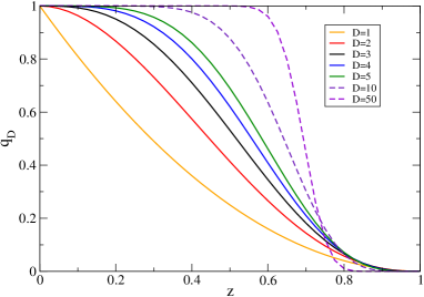
Figure 1: (color online) Reduced partition function $q_{D}(z)$ as a function of $z=\sigma/2R$ for several dimensions. From left to right $D=1,\,2,\,3,\,4,5,10,$ and $50$ last two in dashed line.

Large cavity limit:

The infinitely dilution or large cavity limit $z\rightarrow 0$ (i.e. $\sigma/R\rightarrow 0$) can be studied from the series representation of the reduced partition function $q_{D}(z)$ near $z\simeq 0$,

$$q_{D}(z)=1-z^{D}C_{1,0}+z^{D+1}C_{1,1}+z^{D+3}C_{1,2}+\sum_{k=1}^{\infty}z^{D+3+2k}C_{1,2+k}\;,$$ (52)

where we introduce a set of dimensional dependent constants $\{C\}$ that will denote some power series coefficients through PW. Here, $C_{1,0}=2^{D}$, $C_{1,1}=2^{D}\mathtt{B}_{D}\frac{2D}{D+1}$ and $C_{1,2}=-2^{D}\mathtt{B}_{D}\frac{D(D-1)}{3(D+3)}$. For odd $D$ Eq. (52) is effectively an order $2D$ polynomial. As we will see later, the constant coefficients $\{C_{1,0},\,C_{1,1},\,C_{1,2}\}$ are involved in physical properties of the equivalent many body system. From Eqs. (1) and (18) we obtain

$$Q_{D}=V_{D}^{2}(R)-V_{D}(R)\,2b_{D}+A_{D}(R)\,2a_{D}-J\!\!J_{D}(R)\,2\delta_{D}^{(1)}+O_{D-5}(R)\;,$$ (53)

written in terms of the extensive squared mean curvature $J\!\!J_{D}(R)=A_{D}(R)\cdot(D-1)^{2}\cdot R^{-2}$. The coefficients of area and curvature are

$$a_{D}=b_{D+1}(2\pi)^{-1}\>,$$ (54)

$$\delta_{D}^{(1)}=b_{D+3}\frac{D+1}{D-1}\,(2^{5}3\pi^{2})^{-1}\>,$$ (55)

and $\delta_{D}^{(0)}=0$ corresponds to the absent term proportional to $A_{D}(R)\,R^{-1}$. We may remark that curvature dependence is neither proportional to total nor to Gaussian curvatures, $\mathrm{j}=(D-1)/R$ and $\mathrm{k}=R^{-(D-1)}$ respectively. As may be expected $V_{D}(R)\,2b_{D}$ is the first non ideal correction, and first sign of inhomogeneity and curvature dependence appears in the next two terms. They are deeply connected with $b_{D+j}$ the second cluster integral in higher dimensionality. Therefore, we are showing a direct relation between the -intrinsically inhomogeneous- properties of 2-HS-HWSP and the low density limit properties of HS homogeneous system in higher dimension. Equations (53, 54) and (55) also mixes the properties of systems with odd and even dimensions. Finally, note that Eq. (53) is exact for $D=3$ without the order $D-5$ term Urru and coincidentally $\mathrm{j}^{2}\sim\mathrm{k}$ with the constant value $J\!\!J_{3}(R)=2^{4}\pi$. Further, $J\!\!J_{D}(R)\,\frac{D+1}{D-1}|_{D=3}=J\!\!J_{3}(R)+2K_{3}(R)$ with the extensive gaussian curvature $K_{D}(R)=A_{D}(R)\cdot\mathrm{k}$. Fixing $R=\sigma$ the inner sphere and both particles have the same size and we obtain from Eqs. (6, 53)

$$2\beta_{2}^{vir}\mid_{D=3}=-(2b_{3})^{2}+A_{3}(\sigma)\,2a_{3}-J\!\!J_{3}(\sigma)\,2\delta_{3}^{(1)}\;,$$ (56)

where the second irreducible cluster integral $\beta_{2}^{vir}$ which involves three nodes BookHill , is now written in terms of geometrical measurements of the cavity’s boundary $\{A_{3}(\sigma),\,J\!\!J_{3}(\sigma)\}$ in three dimensions and two body integrals $b_{D}$ in $D\geq 3$. Baus and Colot Baus found $\beta_{2}^{vir}\mid_{D}=-(b_{D})^{2}w_{D}(1/2)$. These type of relations may be interesting for higher order integrals. The three body integral (two HS plus the cavity) $Q_{D}$ and its moments are linked with several three body integrals describing physical properties of the HS inhomogeneous fluid in the low density limit, inside a spherical cavity and even outside a spherical substrate, which will be discussed later in Sec. 6.

Small cavity limit:

Looking at the opposite situation of high density or caging limit we found the final solid, i.e., the densest available configuration of the system. This limiting behaviour has been extensively studied for the HS homogeneous solid system, but also, in small systems Nemeth ; Urru . The caging limit of 2-HS-HWSP is obtained at the root $z=1$. The reduced partition function has an interesting series representation in the neighboring of $z=1$ (valid for $z\leq 1$)

$$q_{D}(z)=(1-z^{2})^{(D+3)/2}C_{2,0}\,(1+C_{2,1}\,(1-z^{2})+O_{2}(1-z^{2}))\;,$$ (57)

with $C_{2,0}=C_{1,1}/(D+3)$, $C_{2,1}=\frac{7-D^{2}}{2(D+5)}$. It shows that CI goes to zero as $(1-z)^{(D+3)/2}$ when system becomes caged. The partition function is then

$$Q_{D}\simeq\sigma^{3(D-1)/2}(R-\sigma/2)^{(D+3)/2}C_{3,0}(1-\sigma^{-1}C_{3,1}(R-\sigma/2)+O_{2}(1-2R/\sigma))\;,$$ (58)

here $C_{3,0}=C_{2,0}\,2^{3-D}(S_{D}/D)^{2}$ and $C_{3,1}=2^{-1}(-9+8\,C_{2,1}+5D)$. Since $Q_{D}$ is identically zero for $R<\sigma/2$ Eq. (58) implies that $Q_{D}$ is non-analytic at $R=\sigma/2$. For odd $D$, the derivative of order $2+(D+1)/2$ and beyond are zero. However, for even $D$ the derivatives of order $2+D/2$ and bigger involves an infinite discontinuity. When a closed system of hard particles is caged as a consequence of the high confinement, the spatial degrees of freedom that becomes lost are related to a zero measure set in the CI integral similar to (1). The consequence is that $Q$ becomes zero, and the signature of the frozen spatial freedom is the order of this root. We introduce the number of spatial lost degrees of freedom $LDF$ and the complementary number of kept degrees of freedom $KDF$, their addition provides the total spatial degrees of freedom $LDF+KDF=N\cdot D$ where $N=2$ is the actual number of particles. We relate $LDF$ with the exponent $(D+3)/2$ in (58). For the studied system of 2-HS-HWSP in the caging limit we obtain

$$LDF=(D+3)/2=1+(D+1)/2\>,$$ (59)

$$KDF=2D-LDF=(D-1)\,3/2\>.$$ (60)

In next sections we will study $LDF$ and $KDF$ in other situations.

3.3 The one body distribution

The one body distribution function are qualitatively similar for all the dimensions and was previously described in detail for $D=2$ and $3$ Urru (Fig.2 therein). A peculiarity of $\rho(r)$ is the plateau of constant density that appears for $R>\sigma$, and which extends from the center to $r=R-\sigma$. For $\sigma/2<R<\sigma$ a null density plateau develops in the range $0<r<\sigma-R$. Therefore, the central plateau density is

$$\rho_{0}=2Q_{D}^{-1}V_{D}\,\left[1-(2z)^{D}\right]=2\left(V_{D}-2b_{D}\right)/Q_{D}\>,$$ (61)

if $R\geq\sigma$, while $\rho_{0}=0$ if $\sigma/2\leq R<\sigma$. Other interesting magnitude is the density at the wall or contact density $\rho_{c}=\rho(r=R)$,

$$\rho_{c}=2V_{D}\,Q_{D}^{-1}\left\{1-\frac{1}{2}\left[w_{D}(1-2z^{2})+(2z)^{D}w_{D}(z)\right]\right\}\>.$$ (62)

These quantities are shown for several dimensions as a function of pore size in Fig. 2. We introduce the rough or mean number density $\bar{\rho}=2/V_{D}(R)$ for comparison. We would like to emphasize that $\rho(r)$ is a discontinuous function at the cavity surface falling down to zero outside the cavity and, also, is non-analytic at $r=Abs(R-\sigma)$. The function $\varrho(r)$ a regularized version of $\rho(r)$ at $r=R$, may be introduced by the short-hand

$$\rho(r)=e_{A}(r)\,\varrho(r)\>,$$ (63)

which must be understood with the help of Eq. (16). It is similar to $\rho(r)$ but includes its analytic continuation for $R\leq r\leq R+\sigma$ and therefore is a smooth function at the hard wall (Hansen , p.166 therein, this procedure was also used in the case of homogeneous fluids, see Eq. (6.11) in Barker ).

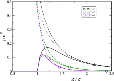
Figure 2: (color online) Characteristic values of density profile. Densities, at the central plateau $\rho_{0}$ (continuous line) and at contact $\rho_{c}$ (dashed line) as a function of pore size. From top to bottom dimensions $D=3,\,5,$ and $7$. Rough density $\bar{\rho}$ for $D=3$ is showed in dotted line.

4 Other Closely Related Systems

It is possible to establish interesting relations between the CPF of 2-HS-HWSP and that of other systems. One of them involves the one stick or dumbbell in the spherical pore, where we think the stick as a rigid body formed by two sticked HS. Other system is that composed by two hard spherical bodies which are constrained to move between the HWSP and an inner hard spherical core. For sufficiently large hard core radius we find the limiting case of 2-HS that are able to move on the surface of a sphere. We may imagine that this system is constituted by two HS sticked to the surface of the HWSP, all immersed in a $D$ dimensional euclidean space. Therefore, it has an effectively reduced dimension of $D-1$. Both systems may be seen as originated in the 2-HS-HWSP and they emerge as a consequence of the addition of a new sticky property. Interestingly, this property is easily introduced by a simple transformation. In PW we will not make a general digression about this transformation, but we simple state that a sticky-bond transformation is performed when one or several of the $e$ or $f$ functions in (1, 18) is transformed in a Dirac delta function or $s$-bond. In a system of many hard bodies in a hard pore a sticky transformation may be done for example by sticking one particle on the surface of the pore, or sticking particles together. The sticky-bond transformation is interesting because in an $N$-body system the most compact spatial configuration, or final solid may be obtained through a series of such operations. It may also mimic a nucleation or condensation process, the adsorption on a surface and even some chemical reactions. In this section the temperature and kinetic factor are not relevant, then we simply make $\Lambda=1$ and then CI and CPF are equal. We may mention that the sticky bond implies that the two bodies must fix their distance, then, even when the concept is related with the adhesive hard sphere bond of Baxter Baxter they are not equivalent.

4.1 The one stick in a HWSP Partition Function

When two HS become stickied together they conform a rigid body because the $s$-bond fix the inter-particle distance to $\sigma$, they form a stick. The sticky-bond transformation may be done by applying the derivative $\partial_{\sigma}$ to $Q_{D}$ on Eqs. (1, 18)

$$Q_{D/b}=C_{b}\,\partial_{\sigma}Q_{D}\>,$$ (64)

the $b$-subindex label means body-particle opposite to point-particle which may be used to describe a HS. The constant $C_{b}=-\sigma^{-(D-1)}$ is found from the large size limit, obtaining

$$Q_{D/b}=S_{D}\,Q_{D}\,\tilde{g}(\sigma)=S_{D}\,V_{D}(R)\,w_{D}(z)\>.$$ (65)

Iterative construction of $w_{D}(z)$ and limits $z\rightarrow 0$ and $z\rightarrow 1$ were described in Section 3.1. Limiting behaviour of the partition function $Q_{D/b}$ is, from Eq. (29)

$$Q_{D/b} = S_{D}V_{D}(R)-A_{D}(R)\,S_{D+1}\sigma(2\pi)^{-1}-J\!\!J_{D}(R)\,S_{D+3}\frac{D+1}{D-1}\sigma^{3}(2^{5}3\pi^{2})^{-1}+O_{D-5}(R)\>,$$ (66)

$$= S_{D}\left(V_{D}(R)-A_{D}(R)\,\sigma\,\mathtt{B}_{D}/D-J\!\!J_{D}(R)\,\sigma^{3}\mathtt{B}_{D}\,(4!D(D-1))^{-1}\right)+O_{D-5}(R)\>,$$ (67)

Note that $V_{D}(R)$ is the volume for one HS particle in the spherical cavity but $Vol=Q_{D/b}/S_{D}$ is the actual volume of the pore for the rigid particle composed by two point particles with fix separation $\sigma$, they are strongly different only for small $R$ in fact

$$\frac{V_{D}(R)-Vol(R)}{V_{D}(R)}=\frac{\sigma}{R}\mathtt{B}_{D}\,\left[1-\left(\frac{\sigma}{R}\right)^{2}\frac{D-1}{4!}\right]+O_{5}(\frac{\sigma}{R})\>.$$ (68)

The first correction to the one HS CPF is related to the Volume coefficient of $Q_{D}$ and the next one relates to the Area coefficient as a consequence of Eqs. (53, 65). The relation may be compactly written $\sigma^{D-1+m}S_{D+m}=2\partial_{\sigma}b_{D+m}$ and is a direct consequence of Eqs. (7, 8). The power at which $Q_{D/b}\rightarrow 0$ .i.e $LDF$ is now, from Eq. (30),

$$LDF=(D+1)/2\>.$$ (69)

When this system becomes caged it conforms a linear rigid rotator. The difference between $LDF$ in Eq. (69) and $LDF$ in Eq. (59) is attributable to the relative distance between both HS. Then we interpret that $LDF$ of $Q_{D}$ corresponds to one degree of freedom from the relative distance between both HS and $(D+1)/2$ corresponding to the $LDF$ of $Q_{D/b}$ related to the rigid rotator degrees of freedom.

4.2 The spherical pore with a hard core

Other closely related system is that of two particle confined in a spherical pore with a fixed central hard core. The main interest to solve this pore shape is the study of the dimensional crossover between $D$ and $D-1$ dimension, which happens when the internal core becomes so large that the two HS may only move on the surface of the $D$-sphere, an effective $D-1$ curved dimensional space. This type of non planar surfaces was introduced by Kratky Kratky in the study of the HS homogeneous systems. Exact results for two, three and four hard particles confined in this non euclidean surface embedded in $D=3$ have been reported calotes . Besides, the 2-HS-HWSP with a hard core (2-HS-HWSP+HC) is by itself interesting cause it is a highly non trivial concave pore. The actual volume of the system is $V_{D}(R)-V_{D}(R-h)$, being $R-h\geq 0$ the radius of the core and $0\leq h<R$. The CI of 2-HS-HWSP+HC was written in Eq. (1) but Eq. (3) must be replaced by $e_{i}=exp[-\beta\psi(r_{i})]=\Theta(R-r_{i})-\Theta(R-h-r_{i})$. Expanding the product of Heaviside functions we obtain

$$Q_{D}(R,h) = S_{D}V_{D}(R)\,\int_{\sigma}^{2R}r^{D-1}w_{D}(r/2R)\,dr+S_{D}V_{D}(R-h)\,\int_{min(\sigma,2(R-h))}^{2(R-h)}r^{D-1}w_{D}(r/2(R-h))\,dr$$ (70)

$$-2S_{D}V_{D}(R-h/2)\,\int_{min(\sigma,2R-h)}^{2R-h}r^{D-1}\zeta_{D}(r/(2R-h),h/(2R-h))\,dr\>,$$

where we have made explicit the conditions on the integration intervals. From them, we observe that CI breaks in three branches depending on $\sigma\leq 2(R-h)$ or $2(R-h)<\sigma\leq 2R-h$ or $2R-h<\sigma\leq 2R$. Last row, also shows that CI separates in two branches according to Eq. (14) depending on $\sigma\leq h$ or not. Equation (70) becomes

$$Q_{D}(R,h) = V_{D}^{2}(R)\,q_{D}(z)+V_{D}^{2}(R-h)\,\Theta(2(R-h)-\sigma)\,q_{D}(\sigma/2(R-h))$$

$$-2V_{D}^{2}(\bar{R})\,\Theta(2R-h-\sigma)\,2^{D}D\,\int_{\tau}^{1}\,y^{D-1}\,w_{D}(y,\Delta)\,dy$$

$$-2\Theta(2R-h-\sigma)\Theta(h-\sigma)\,V_{D}(R-h)(V_{D}(h)-V_{D}(\sigma))\>,$$

being $\bar{R}=R-h/2$ and $\tau=max(\Delta,\sigma/2\bar{R})$. It is clear from Eqs. (4.2, 31) that at each branch $Q_{D}$ is a finite power series in $R$, $h$ and $\sigma$ only for odd dimension. The dimensional systematic of the integral in (4.2) becomes a complex task, then we only analyse with more detail $D=3$ and some characteristics for $D=2,4,$ and $5$. For $D=3$ we evaluate the integral to obtain an explicit expression for the partition function, here we present the result for $\sigma\geq 2(R-h)$,

$$Q_{3}(R,h)=\begin{cases}Vol^{2}-Vol\,2b_{3}+Ar\,2a_{3}-Cur\,2\delta_{3}^{(1)}\>,&\mathrm{if}\>h\geq\sigma\>,\\ \\ Vol^{2}-Vol\,2b_{3}+Ar\,2a_{3}\lambda\,(8-6\lambda+\lambda^{3})/3+\\ -Cur\,2\delta_{3}^{(1)}\lambda^{3}\,(8-9\lambda+2\lambda^{3})\>,&\mathrm{if}\>h<\sigma\>,\end{cases}$$ (72)

where $\lambda=h/\sigma$, and $Vol$, $Ar$ and $Cur$ are the measurements of volume, surface area and boundary quadratic curvature for the actual pore, i.e. $Vol=V_{3}(R)-V_{3}(R-h)$, $Ar=A_{3}(R)+A_{3}(R-h)$ and $Cur=J\!\!J_{3}(R)+J\!\!J_{3}(R-h)=2^{5}\pi$. Noticeable, the partition function is polynomial in each domain, and has continuous second derivative in $h=\sigma$ but a discontinuous third derivative. It is surprising that the volume coefficient $2b_{3}$ and the entire partition function when $h\geq\sigma$ looks exactly equal to $Q_{3}$ (see Eq. (53) and Ref. Urru ) with different Volume, Area, and Curvature measures. We also have established that the central position of the fixed hard core is not essential, first row of Eq. (72) is valid for any internal fixed hard core as long as its boundary is separated from the outer spherical pore wall a distance $\geq\sigma$. The limiting behaviour as $h\rightarrow 0$ to first non null order in $h$ is, from Eq. (72)

$$Q_{3}(R,h\ll\sigma)=h^{2}\left(A_{3}^{2}(R)-A_{3}(R)\,\pi\sigma^{2}\right)+O_{3}(h)=h^{2}S_{3}A_{3}(R)\,\left(R^{2}-(\sigma/2)^{2}\right)+O_{3}(h)\;,$$ (73)

coincidentally $b_{2}=\pi\sigma^{2}$ is equal to the first non ideal gas correction. Here $Q$ goes to zero as $h^{2}$, i.e., the system lost two degrees of freedom. It is an expected property, which must be valid independently of the dimension and even the number of particles, $Q_{D}(R)\simeq h^{N}$ for $R$ large enough. After $h$ goes to zero, $Q/h^{2}$ goes to zero as $\left(R-\sigma/2\right)$ it is the caging limit. In the 2-HS-HWSP in $D=3$, three degrees of freedom are lost when $R\rightarrow\sigma/2$ (see Eqs. (49, 57, 58)) as the system becomes caged, in the spherical pore with an internal core they are lost in two steps.

The study of the systematic dependence on the dimension number of the $h\rightarrow 0$ limit is not easily available from Eq. (70). However, from Eq. (4.2) we find that the partition function for $h\rightarrow 0$ is $Q_{D}=h^{2}Q_{D/s}+O_{3}(h)$ with $Q_{D/s}$ the configuration integral for both HS confined to the surface of the $D$-dimensional sphere also known as the calottes problem calotes . By means of two stick transformation, the $Q_{D/s}$ may be expressed as

$$Q_{D/s}=S_{D}\left.\partial_{R1}\partial_{R2}Q_{D}(R_{1},R_{2})\right|_{R1=R2=R}=S_{D}\left.\partial_{R1}\partial_{R2}\int_{\sigma}^{R1+R2}W_{D}(r,R_{1},R_{2})r^{D-1}\,dr\right|_{R1=R2=R}\>,$$ (74)

where $Q_{D}(R_{1},R_{2})$ is the CI in Eq. (18) but with a different confinement radius for each particle, which is known for $D=2,3$ Urru . Here, we transform the $e_{\mathrm{A}}$, $e_{\mathrm{B}}$ Heaviside functions on Eqs. (1, 17) into Dirac delta functions through the derivatives $-\partial_{Ri}$, sticking both HS on the surface. For practical purposes is much easier to evaluate $Q_{D/s}$ from

$$Q_{D/s}=A_{D}(R)\,S_{D-1}R^{D-1}\int_{0}^{\pi-d}\sin^{D-2}(\theta)\,d\theta\>,$$ (75)

$$Q_{D/s}=A_{D}^{2}(R)\,u_{D-2}(z)\>,$$ (76)

where $A_{D}(R)$ is the system volume and the minimum angular distance between particles is $d=2\arcsin(z)$. Here $u_{D-2}(z)$ is the reduced partition function which plays the same role that $q_{D}$ played in the HWSP, then we define $q_{D/s}(z)\equiv u_{D-2}(z)$. As far as the iterative construction of the $u_{D}(z)$ functions was previously described we present the function for $D=1,\,2,\,3,\,4,$ and $5$

$$q_{1/s}(z)=1\>,$$ (77)

$$q_{2/s}(z)=\frac{2}{\pi}\arccos(z)\>,$$ (78)

$$q_{3/s}(z)=1-z^{2}\>,$$ (79)

$$q_{4/s}(z)=\frac{2}{\pi}\left[\arccos(z)+\sqrt{1-z^{2}}\,z(1-2z^{2})\right]\>,$$ (80)

$$q_{5/s}(z)=1-3z^{4}+2z^{6}\>,$$ (81)

an extra $1/2$ factor must be considered in Eq. (77) due to a kind of ergodic to non-ergodic transition. The asymptotic behavior may be accomplished with the approximate series representations for $q_{D/s}$ Functions

$$q_{D/s}(z)=1-z^{D-1}C_{4}\left[1-\frac{(D-3)(D-1)}{2(D+1)}z^{2}+\frac{(D-5)(D-3)(D-1)}{2^{3}(D+3)}z^{4}+O_{6}(z^{2})\right]\>,$$ (82)

$$q_{D/s}(z)=(1-z^{2})^{(D-1)/2}C_{4}\left[1-\frac{(D-3)(D-1)}{2(D+1)}(1-z^{2})+O_{2}(1-z^{2})\right]\>,$$ (83)

where $C_{4}=\left[\frac{D-1}{2}\,B(\frac{D-1}{2},\frac{D-1}{2})\right]^{-1}$ and truncated terms in Eq. (82) are even powers in $z$. A noticeable characteristic of both series is that they have the same numerical coefficients and both are polynomial with $2(D-2)$ degree for odd dimension. The approximate series for $Q_{D/s}$ are then

$$Q_{D/s}=A_{D}^{2}(R)-A_{D}(R)\,2b_{D-1}+J\!\!J_{D}(R)\,2b_{D+1}\,\frac{D-3}{D-1}(2^{4}\pi)^{-1}-O_{D-5}(R)\>,$$ (84)

where we note that $b_{D-1}=2\pi a_{D-2}$ and the curvature coefficient is $6\pi\delta_{D-2}^{(1)}$ in concordance with Eqs. (54, 55), and

$$Q_{D/s}=\sigma^{3(D-1)/2}C_{5}\,(R-\sigma/2)^{(D-1)/2}\left[1-\sigma^{-1}\frac{(D-1)(7D-9)}{2(D+1)}\,(R-\sigma/2)+\sigma^{-2}O(R-\sigma/2)^{2}\right]\>,$$ (85)

where $C_{5}=2^{2(D-1)}\mathtt{B}_{D}/D$ and the low density limit implies a vanishing curvature limit too. From Eq. (84) we may obtain the first cluster integral correction due to the space curvature for this non euclidean container or spherical boundary conditions. We may compare the first cluster integral in the $(D-1)$-euclidean space $2b_{D-1}$ with the cluster integral in the surface of a sphere in $D$-dimensions $2b_{D/s}=(Q_{D/s}-A_{D}^{2}(R))/A_{D}(R)$, only for $D=3$ we have $2b_{D/s}=2b_{D-1}$, for any dimension we obtain $\underset{R\rightarrow\infty}{\lim}2b_{D/s}=2b_{D-1}$. Partition function for $D=2,\,4,$ and $5$ are

$$Q_{2/s}=A_{2}^{2}(R)-A_{2}(R)\,S_{2}\frac{2R}{\pi}\arcsin(z)\>,$$ (86)

$$Q_{4/s}=(\pi R^{3})^{2}(1-\arcsin(z)+z(1-2z^{2})(1-z^{2})^{1/2})\>,$$ (87)

$$Q_{5/s} = A_{5}^{2}(R)-A_{5}(R)\,\pi^{2}\sigma^{4}/2+A_{5}(R).R^{-2}\pi^{2}\sigma^{6}/12$$ (88)

$$= \left(\frac{4\pi}{3}\sqrt{2}\right)^{2}R^{2}(R-\frac{\sigma}{2})^{2}(R+\frac{\sigma}{2})^{2}(2R^{2}+\sigma^{2})\>.$$

Analyzing the way in which $Q_{D/s}$ goes to zero we obtain from Eq. (83) that,

$$LDF=(D-1)/2=(D+3)/2-2\>,$$ (89)

i.e. two $LDF$ from $Q_{D}$ corresponds to the confinement of both particles on the cavity surface. Now, we are able to extend the results about $LDF$ in $Q_{D}$, $Q_{D/b}$ and $Q_{D/s}$ we may argue that if we stick both particles between them and to the surface we find

$$LDF=(D-3)/2=(D+3)/2-3\>,$$ (90)

where each stick-bond transformation has reduced the $LDF$ on one unit. The idea is that the same final solid-like configuration can be obtained in several ways, but its state properties can not depend on the particular taken path. Therefore, to stick particles between them, next stick each particle to the surface and finally cage the system must produce the same CI (basically the system free energy) that is obtained directly from the caging of the 2-HS-HWSP.

					$D$
Coeff.	Eq.	-1	0	1	2	3	4	5
$S_{D}$	(9)	$-\pi^{-1}$	$0$	$2$	$2\pi$	$4\pi$	$2\pi^{2}$	$8\pi^{2}/3$
$2b_{D}/\sigma^{D}$	(8,53)	$\pi^{-1}$	$1$	$2$	$\pi$	$4\pi/3$	$\pi^{2}/2$	$8\pi^{2}/15$
$2a_{D}/\sigma^{D+1}$	(53)	$-$	$-$	$1/2$	$2/3$	$\pi/4$	$4\pi/15$	$\pi^{2}/12$
$2\delta_{D}^{(1)}/\sigma^{D+3}$	(53)	$-$	$-$	$-$	$1/60$	$\pi/288$	$\pi/378$	$\pi^{2}/1536$
$C_{1,0}$	$2^{D}$	$1/2$	$1$	$2$	$4$	$8$	$16$	$32$
$C_{1,1}$	(52)	$-1/2$	$0$	$1$	$2^{5}/(3\pi)$	$9$	$2^{10}/(15\pi)$	$50$
$-C_{1,2}$	(52)	$0$	$0$	$0$	$2^{4}/(15\pi)$	$2$	$2^{9}/(21\pi)$	$25$
$C_{2,0}$	(57)	$-$	$0$	$1/4$	$2^{5}/(15\pi)$	$3/2$	$2^{10}/(105\pi)$	$25/4$
$C_{2,1}$	(57)	$-$	$7/10$	$1/2$	$3/14$	$-1/8$	$-1/2$	$-9/10$
LDF	(57,58,59)	$1$	$1.5$	$2$	$2.5$	$3$	$3.5$	$4$
$C_{3,0}$	(58)	$-$	$0$	$4$	$2^{6}\pi/15$	$8\pi^{2}/3$	$2^{7}\pi^{3}/105$	$4\pi^{4}/9$
$C_{3,1}$	(58)	$-$	$-17/10$	$0$	$19/14$	$5/2$	$7/2$	$22/5$
$C_{4}$	(82)	$-$	$-$	$1/2$	$2/\pi$	$1$	$16/(3\pi)$	$3$
$C_{5}$	(85)	$-$	$1$	$1/2$	$4/\pi$	$4$	$128/(3\pi)$	$48$

Table 1: Several constant coefficients of the series representation of CIs and other functions. Some values for $D=-1$ and $0$ correspond to a suitable limiting behavior.

5 Mechanical equilibrium and Pressure tensor

To make a more complete and microscopic characterization of the system it is necessary to evaluate the pressure tensor. Briefly, pressure tensor, density and external potential are related as a consequence of the mechanical equilibrium by

$$\nabla\cdot\mathbf{P}+\rho\nabla\psi=0\>,$$ (91)

where the explicit position dependence of the magnitudes has been dropped. In any inhomogeneous system the tensor can be split into

$$\mathbf{P}=\beta^{-1}\rho\,\mathbf{Id}+\mathbf{P}^{U}\;,$$ (92)

where $\mathbf{Id}$ is the $D\times D$ identity matrix and $\mathbf{P}^{U}$ is the interaction part of the tensor Mor . In systems with spherical symmetry $\mathbf{P}^{U}$ is diagonal with only two different components Blok1 ; Poni the normal and tangential components $P_{N}^{U}$ and $P_{T}^{U}$

$$\mathbf{P}^{U}=P_{N}^{U}\hat{\mathbf{r}}\hat{\mathbf{r}}+P_{T}^{U}(\hat{\boldsymbol{\varphi}}\hat{\boldsymbol{\varphi}}+\hat{\boldsymbol{\theta}}_{1}\hat{\boldsymbol{\theta}}_{1}+...+\hat{\boldsymbol{\theta}}_{D-2}\hat{\boldsymbol{\theta}}_{D-2})\;,$$ (93)

where $\hat{\boldsymbol{\varphi}},\hat{\boldsymbol{\theta}}_{1},...,\hat{\boldsymbol{\theta}}_{D-2}$ are the angular versors. Then, for systems with spherical symmetry Eq. (91) may be written as

$$\partial_{r}P_{N}+\frac{D-1}{r}(P_{N}-P_{T})+\rho\partial_{r}\psi=0\>.$$ (94)

Further simplifications apply to a hard wall container, there $\rho(r)$ is discontinuous at $r=R$ but $\varrho(r)$ is not (see Eq. (63)), we obtain from Eq. (94)

$$\partial_{r}P_{N}+\frac{D-1}{r}(P_{N}-P_{T})=-\beta^{-1}\delta(r-R)\,\varrho\>,$$ (95)

$$\partial_{r}P_{N}^{U}+\frac{D-1}{r}(P_{N}^{U}-P_{T}^{U})=-\beta^{-1}e_{\mathrm{A}}(r)\,\partial_{r}\varrho\>,$$ (96)

both equations are equivalent to Eq. (94) and then necessary conditions for an acceptable pressure tensor definition. Nevertheless they are formally strongly different. The inhomogeneous term in the differential equation (95) shows at the boundary a divergent singular contribution to the total pressure components with zero contribution from positions inside and outside the boundary. Although, inhomogeneous term in Eq. (96) shows at the boundary a discontinuous singular contribution to $P^{U}$ components, with non zero contribution from inside points. We will regress to this issue in a forthcoming paragraph.

Turning now to the interaction part of pressure $P^{U}$, is known that its detailed expression is non unique. Particularly, different possible definitions of $P^{U}$ produce different values of pressure tensor in inhomogeneous fluids Blok1 . In this work we adopt a pressure tensor definition extensively utilized in MD simulations Mor , the components of the pressure tensor for the two body system are

$$P_{ab}^{U}(r)\equiv\left\langle r_{\mathrm{AB}}^{a}F_{\mathrm{AB}}^{b}(\mathbf{r}_{\mathrm{AB}})\delta(\mathbf{r}-\mathbf{r}_{\mathrm{A}})\right\rangle\>,$$ (97)

been $r^{a}=\mathbf{r}\cdot\hat{\mathbf{a}}$ and $F_{\mathrm{AB}}^{b}(\mathbf{r})=-\frac{d\phi}{dr}\frac{r^{b}}{r}$ the component of the force between particles in the $\hat{\mathbf{b}}$ direction (see Eq. (3.20) in Ref. Mor ). It has been argued that Eq. (97) can be obtained from the Irving Kirkwood pressure tensor with the assumption of short range interaction Mor . Interestingly, the adopted definition for the pressure is an intrinsic two bodies emergent property which depends only on the position of two particle coordinates and does not depend on any choice of an integration path. In the present problem is important to notice that position of both bodies are the point of pressure evaluation $\mathbf{r}=\mathbf{r}_{\mathrm{A}}$ and the integrated position $\mathbf{r}_{\mathrm{B}}$ in the mean value of Eq. (97). It is a desirable property of $\mathbf{P}^{U}(\mathbf{r})$ in any few body system that the microscopic configurations with zero probability to find a particle in position $\mathbf{r}$ must not contribute to the pressure. This property is not accomplished by the Irving-Kirkwood choice for the pressure tensor. Equation (97) may be written as

$$P_{ab}^{U}(r)=(\beta Q_{D})^{-1}e_{\mathrm{A}}(r)\intop e^{\prime}_{\mathrm{AB}}e_{\mathrm{B}}\frac{r_{\mathrm{AB}}^{a}r_{\mathrm{AB}}^{b}}{|r_{\mathrm{AB}}|}d\mathbf{r}_{\mathrm{B}}\>,$$ (98)

where $\mathbf{r}_{\mathrm{AB}}=\mathbf{r}-\mathbf{r}_{\mathrm{B}}$ and $e^{\prime}_{\mathrm{AB}}=\delta(r_{\mathrm{AB}}-\sigma)$. Changing the integration variable to $\mathbf{r}_{\mathrm{AB}}$ and integrating over the radial coordinate one gets

$$P_{ab}^{U}(r)=(\beta Q_{D})^{-1}\sigma^{D}e_{\mathrm{A}}(r)\intop e_{\mathrm{B}}(r_{\mathrm{B}})\hat{r}_{\mathrm{AB}}^{a}\hat{r}_{\mathrm{AB}}^{b}d\Omega_{\mathrm{AB}}\>,$$ (99)

with $r_{\mathrm{B}}=\left|\mathbf{r}-\sigma\,\hat{\mathbf{r}}_{\mathrm{AB}}\right|$ and $\hat{r}^{b}=\hat{\mathbf{r}}\cdot\hat{\mathbf{b}}$. The two independent components of this tensor are

$$P_{N}^{U}(r)=(\beta Q_{D})^{-1}e_{\mathrm{A}}(r)\,\sigma^{D}S_{D-1}\,\intop e_{\mathrm{B}}\cos^{2}\theta\sin^{D-2}\theta\,d\theta\>,$$ (100)

$$P_{T}^{U}(r)=(\beta Q_{D})^{-1}e_{\mathrm{A}}(r)\,\sigma^{D}S_{D-1}(D-1)^{-1}\,\intop e_{\mathrm{B}}\sin^{D}\theta\,d\theta\>,$$ (101)

where the integration interval $(0,\pi)$ may be reduced to $(\theta_{min},\pi)$ by the effect of $e_{\mathrm{B}}$, with $\theta_{min}=0$ if $r<R-\sigma$, $\theta_{min}=\pi$ if $|r-\sigma|>R$, and $\theta_{min}=\pi-\arccos(-R^{2}+\sigma^{2}+r^{2})/(2r\sigma)$ otherwise. Both integrals expressed in terms of known functions are

$$P_{N}^{U}(r)=(\beta Q_{D})^{-1}e_{\mathrm{A}}(r)\,2^{-1}V_{D}(\sigma)\>\left[D\,w_{D-2}(\cos\alpha)-(D-1)\,w_{D}(\cos\alpha)\right]\>,$$ (102)

$$P_{T}^{U}(r)=(\beta Q_{D})^{-1}e_{\mathrm{A}}(r)\,2^{-1}V_{D}(\sigma)\>w_{D}(\cos\alpha)\>,$$ (103)

where $\cos\alpha=1$ if $r>R+\sigma$, $\cos\alpha=-sign(R-\sigma)$ if $r<R-\sigma$ and $\cos\alpha=(-R^{2}+\sigma^{2}+r^{2})/(2r\sigma)$ if $R-\sigma\leq r\leq R+\sigma$. Figure 3 shows both pressure tensor components as a function of position into the cavity. We observe that when the pore is big enough, $R>\sigma$, a pressure plateau develops at the center of the pore in the range $0\leq r<R-\sigma$. In the region $R-\sigma\leq r<R$ the inhomogeneous pressure region develops. The shape of pressure tensor and density profiles are simply correlated (see Fig. 2 in Urru ), their constant value plateau and inhomogeneous regions coincide, even more, when plateau density becomes null, pressure goes to zero too.

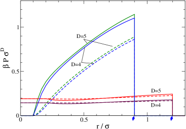
Figure 3: (color online) Pressure tensor components. Continuous line corresponds to $P_{N}$ and dashed line to $P_{T}$. Two cavity sizes $R/\sigma=0.9$ and $R/\sigma=1.2$, and two different dimension $D$ are shown. The arrows indicate $R/\sigma$ values.

In the homogeneous region the normal and tangential components of the pressure tensor become equal, and the pressure tensor reduces to a constant scalar pressure $P_{0}$ Blok1 . In this case Eqs. (102, 103) lead to

$$P_{N,T}^{U}(0)=P_{0}^{U}=(\beta Q_{D})^{-1}2b_{D}\>,$$ (104)

finally, according to Eq. (92) the pressure in the homogeneous density plateau is

$$\beta P_{0}=\rho_{0}+\frac{2b_{D}}{Q_{D}}=2(V_{D}-b_{D})/Q_{D}\>,$$ (105)

for $R\geq\sigma$ while $\beta P_{0}=0$ for $\sigma/2\leq R<\sigma$. The value of the pressure tensor at contact can be obtained from Eqs. (102, 103) with $r=R$ and $\cos\alpha=z=\sigma/(2R)$ but no further simplification may be done. In Fig. 4 we plotted the characteristic values of the pressure tensor. There we can observe that the maximum of $P_{0}$ is attained at smaller $R$ than the maximum of the density (see Fig. 2).

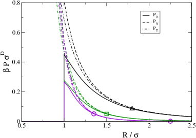
Figure 4: (color online) Characteristic values of pressure tensor. Pressure, at the central plateau $P_{0}$ (continuous line) and contact value ($r=R$) of both components $P_{N}$ and $P_{T}$ (dashed line and dash-dotted line) as a function of pore size. From top to bottom dimensions $D=3,\,5,$ and $7$ in triangles, squares and circles.

We have verified that in the inhomogeneous region $abs(R-\sigma)\leq r\leq R$, Eq. (96) with $P_{N,T}$ from Eqs. (102, 103) is false. Two probable reasons may be argued, the invalid short range hypothesis for the HS potential for nonuniform density, and/or the incorrect pressure tensor definition of Eq. (97) due to the hard wall boundary condition (see Eq.(3.5) in Poni ). As far as the mechanical equilibrium of Eq. (96) is still valid in the homogeneous plateau, and pressure should not strongly depend on the definition details in this region, we accept the validity of the obtained pressure tensor for $0<r<abs(R-\sigma)$. It is particularly interesting to analyse the point $r=R$ where we find $\partial_{r}\varrho>0$. We may note that the discontinuous behaviour of $P_{N}^{U}$ (but not of $P_{T}^{U}$) at $r=R$ violates Eq. (96). The existence of the Heaviside factor $e_{A}(r)$ on the right hand side of Eq. (96) must be balanced with the same global factor at the left side, and forbids the appearance of an uncompensated Dirac delta. However, the derivative of a discontinuous $P_{N}^{U}$ just produce a singular Dirac delta at $r=R$. If we assume the validity of this equation one obtains that the discontinuity is completely unphysical. Thus, we need the continuity of the interaction normal component of the pressure tensor to overcome the mismatch.

6 The Equation of state and the Laplace Equation

We are interested in the equation of state (EOS) of the 2-HS-HWSP, i.e. the thermodynamic description of the complete inhomogeneous system. We adopt a point of view usually taken in spherical droplets which makes a description in terms of the properties in the homogeneous regions of the system. In this section we drop any explicit unnecessary $D$ subindex and dependence on cavity size $R$, then $V=V_{D}(R)$, $Q=Q_{D}(R)$ and so on. The properties in the homogeneous region may be found from Eqs. (61, 105). From these Eqs., for $R>\sigma$ we obtain

$$\frac{\beta P_{0}}{\rho_{0}} = 1+\frac{b}{2}\,\frac{\bar{\rho}}{1-b\bar{\rho}}\>,$$ (106)

$$= 1+\frac{1}{2}\,(V/2b-1)^{-1}\>,$$ (107)

where the compressibility factor at the constant density plateau is a simple function of $\bar{\rho}$ or $V$. We may note that both expressions diverge at $R=\sigma$ and $V=2b$. For this pore size the plateau of constant density vanishes and $\rho_{0}=0$. Interestingly, in Eq. (107) we have found the bulk van der Waals EOS without the attractive term, the only flavor remaining the two body system is a $1/2$ factor. Owing to Eq. (106) does not depend on geometrical parameters which resembles the cavity’s spherical symmetry it should be valid also for 2-HS confined in pores with other geometries. In Eqs. (106, 107) $P_{0},\>\rho_{0}$ and $\bar{\rho}$ (or $V$) are not independent variables, even, they are functions of system’s size $R$. The Eq. (106) can be written in two forms which resemble the contact theorem for the bulk homogeneous HS system (see Eq. (2.5.26) in Hansen and also Reiss )

$$\beta P_{0} = \rho_{0}+b\bar{\rho}^{2}\,\frac{g(\sigma)}{w(z)}\>,$$ (108)

$$= \rho_{0}+\frac{b}{2}\rho_{0}^{2}\,\frac{q(z)}{(1-2z)^{2}}\>,$$ (109)

where in fact $g(\sigma)/w(z)=(2q(z))^{-1}$ and then $g(\sigma)/w(z)\rightarrow 1/2$ when $R\rightarrow\infty$. The Eqs. (108, 109) make sense only for $0\leq z<1/2$ or $\sigma<R\leq\infty$, where for the smallest pore ($R=\sigma$ and $z=1/2$) $\rho_{0}=0$. In such a case, the term which multiply $\bar{\rho}^{2}$ in Eq. (108) takes a finite value, but, the term which multiply $\rho_{0}^{2}$ in Eq. (109) diverges. However, Eq. (109) goes to zero. This shows an only apparent different behaviour, because Eqs. (108, 109) are different representations of the same equation. At large $R$ the overall and plateau densities are related by

$$\rho_{0}\simeq\bar{\rho}-\frac{a}{2}\,\bar{\rho}^{3}A(R)\simeq\bar{\rho}-C_{6}\,\bar{\rho}^{2+1/D}\>,$$ (110)

with $C_{6}=(D^{D-1}2^{-1}S_{D})^{1/D}a_{D}$ and $A(R)\sim\rho_{0}^{-(D-1)/D}\sim\bar{\rho}^{{}^{-}(D-1)/D}$ for $D>1$. Polynomial expressions for the pressure as a function of density, may be found by considering the firsts terms of $P_{0}$ as a density power series

$$\beta P_{0} \simeq \rho_{0}+\frac{b}{2}\rho_{0}^{2}+\frac{b^{2}}{2}\rho_{0}^{3}+\frac{b}{4}\,\rho_{0}^{4}\left(2b^{2}+a\,A(R)\right)\>,$$ (111)

$$\simeq \bar{\rho}+\frac{b}{2}\,\bar{\rho}^{2}+\frac{1}{2}\bar{\rho}^{3}\left(b^{2}-a\,A(R)\right)\>.$$ (112)

Here we choose two density parametrization, the plateau density and rough density, $\rho_{0}$ and $\bar{\rho}$ respectively. The expansions in Eqs. (111, 112) end at the order of the first signature of the inhomogeneity. Both equations show that the first correction to the ideal gas behaviour is positive and involves the expected closed system correction Hub . Besides, the Eqs. (111, 112) involve terms with higher powers in the density than two. This feature may sound conflicting in a two body system, but in fact, it is a direct consequence of the fixed number of particles that characterizes the Canonical Ensemble approach. In Fig. 5 we plot the pressure in the homogeneous plateau as a function of both density parameters. In Fig 5 (a) we adopt the plateau density $\rho_{0}$. There, an important characteristic is apparent, for small cavities $\sigma/2<R<\sigma$ we obtain $\rho_{0}=0$ and $P_{0}=0$ (see also Figs. 2 and 3). The anomalous bi-valued behaviour of $P_{0}(\rho_{0})$ is a consequence of the non monotonic behavior of the density in the homogeneous region as was shown in Fig. 2. In Fig. 5 (b) we adopt the rough density $\bar{\rho}$. For $P_{0}(\bar{\rho})$ we find a simpler general dependence with a monotonic behaviour until $\bar{\rho}=2/V(1)$ is reached. Note that the maximum attainable density is $\bar{\rho}_{max}=2/V(1/2)$. In both Figs. 5 (a) and (b) the pressure attains its maximum when the density plateau disappears at $R=\sigma$ and then pressure drops discontinuously to zero.

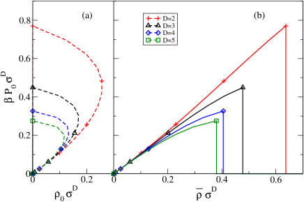
Figure 5: (color online) Pressure in the homogeneous plateau. From top to bottom $D=2,3,4,$ and $5$. Two different choices of density parameter are depicted. At left hand side (a), in dashed line we adopt the $\rho_{0}$ as density parameter. At right hand side (b), in continuous line we adopt the rough density $\bar{\rho}$.

Interestingly, both used density parameters $\{\rho_{0},\bar{\rho}\}$ are usually utilized to describe the behaviour of macroscopic fluid systems. From an opposite point of view, we may concentrate in the external force and on contact properties. From the wall theorem Blok3 ; Lovet the total scalar force between the wall and the HS system in a pressure form is

$$d_{R}\ln(\tilde{Q})\cdot A(R)^{-1}=\beta P_{W}=\rho_{c}\>,$$ (113)

with $\rho_{c}$ from Eq (62). The general features of $\beta P_{W}(R)$ for $D=2$ and $3$ can be seen in Fig. 1 of Ref. Urru . There, the basic systematic behaviour with increasing dimensionality is apparent. As a consequence of the chain rule of the derivative and the sticky bond transformation the numerator of $\rho_{c}$ is the CI of one HS in a diminished volume. The allowed volume for the HS particle is the free volume available when the other HS is sticked to the surface. The asymptotic behaviour of $P_{W}$ may be obtained from Eqs. (53, 58). For $D=2$ and $3$ it was studied in Urru . In the caging limit, when $R\rightarrow\sigma/2$, $P_{W}$ diverges as

$$\beta P_{W}\simeq\frac{D+3}{2\,A(\sigma/2)}\,(R-\frac{\sigma}{2})^{-1}\>,$$ (114)

$$\frac{\beta P_{W}}{\bar{\rho}}\simeq\frac{D+3}{4D}\,(V/V_{0}-1)^{-1}\>,$$ (115)

where $V_{0}=V(\sigma/2)$ and the expressions in Eqs. (114, 115) are consistent to order minus one in $(R-\frac{\sigma}{2})$ and $(V/V_{0}-1)$. The same power dependence of the compressibility factor was found for the caging limit of N-HS systems under periodic boundary conditions Sals . A comparison between Eqs. (107) and (115) shows an interesting similarity at $D=3$.

Finally, we shall study the surface tension of the system. Due to the failure of the obtained pressure tensor we can not evaluate a microscopic expression for the surface tension, however we may adopt a macroscopic approach. Identifying the radius of the dividing interface with $R$ we define $\tilde{\gamma}$ by

$$\beta\mathrm{j}\tilde{\gamma}(R)=\rho_{c}-\beta P_{0}=\beta\Delta P\>,$$ (116)

where at the left hand side appears the pressure difference $\Delta P=P_{W}-P_{0}$. If we identify $\tilde{\gamma}$ with the surface tension, the Eq. (116) is the original version of Laplace equation applied to a spherical substrate-fluid interface Blok3 . Besides, for $D=1$ or $R\rightarrow\infty$ we obtain the planar equilibrium condition $\rho_{c}=\beta P_{0}$. Figure 6 shows $\tilde{\gamma}$ for different radii and several dimensions $D>1$. Some general features are: it is a positive defined quantity; at large $R$ the value of $\tilde{\gamma}$ goes to zero with an expected power law dependent on $D$; in the opposite, as $R/\sigma\rightarrow 1/2$ $\tilde{\gamma}$ increases indefinitely as $\rho_{c}$ do. It can be observed a finite jump at $R/\sigma=1$ due to a discontinuity in $P_{0}$. Probably such discontinuities in $P_{0}$ and $\tilde{\gamma}$ are unphysical artifacts of the adopted definition for $P_{ab}^{U}(r)$.

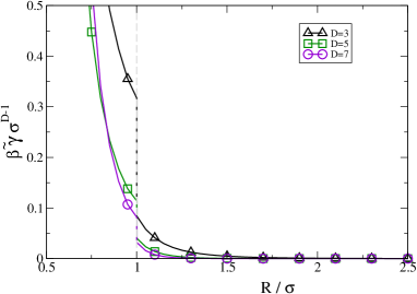
Figure 6: (color online) Function $\tilde{\gamma}$, its dependence on pore radius for several dimensions. The dashed line shows the discontinuity at $R/\sigma=1$.

For $R>\sigma$ we have

$$\beta\mathrm{j}\tilde{\gamma} = 2\left[V-(1-c(z))\,b-V+b\right]/Q\>,$$ (117)

$$= 2b\,c(z)/Q\>,$$

$$c(z)=1-w_{D}(z)-(2z)^{-D}w_{D}(1-2z^{2})\>,$$ (118)

where $0<c(z)<1$ and the most relevant terms of $c(z)$ are

$$c(z)\simeq(D-1)\,\mathtt{B}_{D}z\,\left[2(D+1)^{-1}-\frac{D-3}{3(D+3)}z^{2}\right]\>,$$ (119)

where for $D=3$ we obtain the somewhat surprising result $c(z)=z\,3/4$. To first non null order in density and curvature we obtain

$$\beta\tilde{\gamma}\simeq\frac{a}{2}\bar{\rho}^{2}-\mathsf{\delta}_{D}^{(1)}2^{-1}(D-1)(D-3)\,R^{-2}\bar{\rho}^{2}\>,$$ (120)

where first term does not show any curvature dependence. In Addition, to the same order of accuracy in density we may replace $\bar{\rho}\rightarrow\rho_{0}$. We identify the first density-non-curvature term as $\beta\gamma_{flat}=a/2\,\bar{\rho}^{2}$. To first non null order we obtain

$$\tilde{\gamma}/\gamma_{flat}-1\simeq-\left(\frac{\sigma}{R}\right)^{2}\,\frac{(D-3)(D+1)}{24\,(D+3)}\>,$$ (121)

where the right hand term becomes null for $D=3$. Unfortunately $\tilde{\gamma}$ is not the surface tension but in fact it is an excess free work. A better proposal for the definition of the surface tension $\gamma$ is a refined version of the Laplace equation Hend2

$$\partial_{R}\gamma+\mathrm{j}\gamma=\Delta P\>,$$ (122)

where $\Delta P=\mathrm{j}\tilde{\gamma}$. Definition from Eq. (122) separates an explicit curvature dependent term from $\Delta P$ Blok3 . The asymptotic behaviour of $\Delta P$ is essentially described in Eq. (120), from that we obtain for the surface tension

$$\gamma/\gamma_{flat}-1\simeq-\left(\frac{\sigma}{R}\right)^{2}\,\frac{(D-1)(D+1)}{24\,(D+3)}\>,$$ (123)

where now, the right hand term becomes null at $D=1$. We may study the same system from a different radii which is an interesting point of view principally for non sharp interfaces usually found in fluid droplets. Being $R^{\prime\prime}=R+\varepsilon$ and following Henderson Hend2 we define,

$$\mathrm{j}(R)\,\beta\gamma(R)=\mathrm{j}(R^{\prime\prime})\,\beta\gamma(R,R^{\prime\prime})+\beta\partial_{R^{\prime\prime}}\gamma(R,R^{\prime\prime})\>,$$ (124)

its solution is

$$\beta\gamma(R,R^{\prime\prime})=\beta\gamma(R)\,\frac{1}{D}\left\{(D-1)\,\left(\frac{R}{R^{\prime\prime}}\right)^{-1}+\left(\frac{R}{R^{\prime\prime}}\right)^{D-1}\right\}\>,$$ (125)

and then

$$\gamma(R,R^{\prime\prime})/\gamma(R)-1=\frac{D-1}{2}\,\left(\frac{\varepsilon}{R}\right)^{2}+O_{3}(\frac{\varepsilon}{R})\>,$$ (126)

showing that first correction is second order in $\varepsilon/R$ and positive for $D>1$.

We expect that, several of the above expressions may be generalized for any number of particles $N$ with the addition of the overall $N$-dependent correction factor Hub . Here we do not demonstrate but merely suggest that, the Eq. (120) should be multiplied by $2(1-N^{-1})$ at right hand side Kratky to become valid to the same order in density and curvature. The same modification applies to $\gamma_{flat}$. However, this prefactor does not modify the ratios in Eqs. (121, 123). Therefore, for a large enough $R$ we obtain for the $N$-HS-HWSP system in $D$ dimensions

$$\beta\gamma_{flat}\simeq a\,(1-N^{-1})\bar{\rho}^{2}\>,$$ (127)

$$\gamma/\gamma_{flat}-1\simeq-\left(\frac{\sigma}{R}\right)^{2}\,\frac{(D-1)(D+1)}{24\,(D+3)}\>,$$ (128)

both are new results even in the most interesting case of $D=3$. Furthermore, the Eq. (127) represents the first term of the density power series of the surface tension for any hard wall cavity. In addition, Eq. (128) applies too for the conjugate system of a hard wall spherical core surrounded by a HS fluid. Finally, we are interested in establish some relations between the studied system and the open (grand canonical ensemble) system of HS in contact with a hard spherical wall. The low density limit of an inhomogeneous open system was studied by Bellemans and Sokolowski-Stecki Bell ; Soko who found the surface tension virial series and apply it to the HS system in contact with a planar hard wall (cite I Ref. Bell and I, III Ref. Soko ) and contained in a HWSP (cite III in Ref. Bell ) in $D=3$. In the HS inhomogeneous fluid in a HWSP the $\gamma$ first power density coefficient and zero order in curvature is the same that appears when a planar wall is studied (from Area term in Eq.(53)) $\beta_{\Omega 2}^{Bell}=W_{2}^{S-S}/A_{D}(R)=a_{D}=b_{D+1}(2\pi)^{-1}$ which may be found by taking $N\rightarrow\infty$ at Eq. (127). The first curvature correction of this should be $\mathsf{\delta}_{D}^{(0)}$. Bellemans obtained that in three dimensions this constant is null, $\mathsf{\delta}_{\Omega 2}^{Bell}=\mathsf{\delta}_{3}^{(0)}=0$, and we obtain $\mathsf{\delta}_{D}^{(0)}=0$ for $D\geq 2$ (from the nonexistent $R^{D-2}$ term in Eq.(53)), whereas the first non null curvature correction is $\mathsf{\delta}_{D}^{(1)}$ (from $R^{D-3}$ curvature term in Eq. (53)). To our best knowledge, all this properties have been never studied or evaluated for $D\neq 2$ and $3$ Bell ; McQ ; Soko ; Urru , and here we are showing the systematic dimensional dependence in terms of the second cluster integral coefficient in a higher dimensionality space (see Eq. (55)). Concisely, Eq. (4.5) in III Ref. Bell for a $D$ dimensional system must be written as

$$\gamma/\gamma_{flat}-1 = -\mathrm{j}^{2}\frac{\mathsf{\delta}_{D}^{(1)}}{a_{D}}+O_{4}(R^{-1})+O(\rho)\,O(R^{-1})\>,$$ (129)

$$\simeq -\left(\frac{\sigma}{R}\right)^{2}\,\frac{(D-1)(D+1)}{2^{3}3\,(D+3)}\>.$$

where now $\gamma_{flat}$ is the surface tension of the open system in contact with a planar wall. An interesting fact is that first correction is then quadratic in curvature and zero order in density. Besides, for a HS fluid in contact with a hard convex spherical wall (sometimes referred in the literature as a spherical cavity inside of the bulk fluid) this first order curvature correction should be exactly the same. The term proportional to $-R^{-2}$ in Eq. (129) is $1/40$ and $1/18$ for $D=2$ and $3$ respectively and becomes greater than one for $D\geq 27$. A consequence of Eq. (129) is that the Tolman length of the athermal system of HS-HWSP scales as $\delta^{Tol}\sim\rho$ for low density. It seems that the study of the three particle system will provide the value of the proportionality constant. We may conclude this section by noting that a curvature correction proportional to $\sigma/R$ should exist at Eqs. (121, 128) if we consider a somewhat more realistic potentials with soft repulsion and/or attractive well.

Here, we have presented an study of the bulk properties of a system consisting in 2HS-HWSP. In such an analysis we followed deliberately a non-thermodynamic approach. Even when it may be unexpected, the direct derivation of properties such as the pressure and surface tension using a thermodynamic approach is not a simple task Urru2 . The full implementation of this path requires a careful evaluation of several problems related with the nonextensivity of the system. This subject will be analyzed in an incoming work.

7 Final remarks

The few body system consisting of two hard spheres in a spherical pore in any dimension has been studied in the framework of the canonical ensemble of statistical mechanics. It was showed that several properties of such an inhomogeneous spherical system can be exactly evaluated. Analytical exact expressions for the canonical partition function $\tilde{Q}_{D}$, density distribution function $\rho(r)$, and pressure tensor $\mathbf{P}(r)$ were obtained. The iterative construction of these functions in terms of the same properties for dimensions lower than $D$ was performed. We should emphasize that neither approximations nor power series truncation were done along these derivations. The study of the analytical properties of CI at the low density limit or large $R$ value, and the highly confinement limit or final solid were analysed. We found that properties at both limits are correlated. This becomes clear for odd $D$ values where the CI is a polynomial and low density limit involves high order $R$ monomials, though caging limit properties relates with the degree of the zero of CI at $R=\sigma/2$. We found that such zero is of order $(D+3)/2$.

Other systems which are closely related to the 2-HS-HWSP have been also analysed. The system of two sticky HS or rigid linear body into a spherical pore was tackled. The two HS into a spherical pore with a smaller internal and fixed hard core was studied with special emphasis in the limit of on surface confinement. Several exact relations between the three closely related systems were established by applying the sticky bond transformation which makes possible their unified study. It was examined the way in which properties of the three systems become strongly dependent on the low density regime and on the opposite caging limit. Several equations that relates the coefficients of these systems were obtained.

The pressure tensor of the 2-HS-HWSP was investigated. The re-examination of the mechanical equilibrium condition for a system with a hard spherical boundary was done. New constraints between non ideal pressure tensor components and one body distribution function slope at contact with the curved wall was obtained. The analytical evaluation of one possible definition of the pressure were performed. The obtained expression disregards the former equilibrium condition and therefore the used pressure tensor definition must be considered incorrect or at most approximate.

The EOS of 2-HS-HWSP system was studied. We have analytically evaluated the pressure-density relation and the surface tension. In connection with the open system of HS in a HWSP, our results are consistent with that obtained by Bellemans Bell the first correction in the surface tension due to the curvature in the confining surface is not of order $R^{-1}$ in three dimension. We also show (see Eqs. (53, 55) and (129)) that the first correction has order $R^{-2}$ independently of the system’s dimensionality and is zero order in density. In addition we determined the value of the coefficients corresponding to the first inhomogeneous and first non planar wall corrections for all dimensions, Eqs. (54, 55). To the best of our knowledge, it is the first time that both coefficients are evaluated.

The In-Out relation introduced in Ref. Urru and described in Section 2, the stick transformation introduced in Section 4, and several results (e.g., Eqs. (53, 66, 72) and (84)) suggest interesting links with the mathematical theory of Convex Bodies also known as Integral Geometry Meck ; Muld that will be studied in future works.

Appendix A Appendix: Properties of $w_{D}(y,\Delta)$

This appendix is devoted to the iterative construction of $w_{D}(y,\Delta)$. The procedure to iteratively build $w_{D}(y,\Delta)$ is traced from Eqs. (23, 31) where the last one applies only for $\Delta\leq y\leq 1$. We define the complementary function of $w_{D}(y,\Delta)$ (see Eq. (31)), $\widetilde{w}_{D}(y,\Delta)$

$$\widetilde{w}_{D}(y,\Delta)\equiv\frac{1}{2}\left(1+\Delta\right)^{D}w_{D}(x^{\prime})-\frac{1}{2}\left(1-\Delta\right)^{D}w_{D}(x^{\prime\prime})\>.$$ (130)

with $x^{\prime}=r^{\prime}/2R_{1}=(y^{2}+\Delta)/[y\,(1+\Delta)]$ and $x^{\prime\prime}=r^{\prime\prime}/2R_{2}=(y^{2}-\Delta)/[y\,(1-\Delta)]$. From the definition of $w_{D}(y,\Delta)$ (31), replacing $w_{D}(x)$ with the aid of Eq. (23) and rearranging terms we obtain

$$w_{D}(y,\Delta) = (1+\Delta^{2})w_{D-2}(y,\Delta)+2\Delta\,\widetilde{w}_{D-2}(y,\Delta)-$$ (131)

$$\left(\left(\frac{R_{1}}{\bar{R}}\right)^{D}x^{\prime}(1-x^{\prime 2})^{(D-1)/2}+\left(\frac{R_{2}}{\bar{R}}\right)^{D}x^{\prime\prime}(1-x^{\prime\prime 2})^{(D-1)/2}\right)\mathtt{B}_{D}/D\>,$$

Following a similar approach with Eq. (130) and writing $\{R_{1},R_{2}\}$ in terms of $y$ and $\Delta$ we obtain the iterative relations

$$w_{D}(y,\Delta) = (1+\Delta^{2})w_{D-2}(y,\Delta)+2\Delta\,\widetilde{w}_{D-2}(y,\Delta)-$$ (132)

$$y^{2-D}\left((1-y^{2})(y^{2}-\Delta^{2})\right)^{(D-1)/2}2\mathtt{B}_{D}/D\>,$$

$$\widetilde{w}_{D}(y,\Delta) = 2\Delta\,w_{D-2}(y,\Delta)+(1+\Delta^{2})\widetilde{w}_{D-2}(y,\Delta)-$$ (133)

$$\Delta\,y^{-D}\left((1-y^{2})(y^{2}-\Delta^{2})\right)^{(D-1)/2}2\mathtt{B}_{D}/D\>.$$

First functions of the series are

$$w_{-1}(y,\Delta)=1/(1-\Delta^{2})\;,$$ (134)

$$\widetilde{w}_{-1}(y,\Delta)=-\Delta/(1-\Delta^{2})\;,$$ (135)

$$w_{0}(y,\Delta)=\frac{1}{\pi}\,\left[arccos(\frac{y^{2}+\Delta}{y(1+\Delta)})+arccos(\frac{y^{2}-\Delta}{y(1-\Delta)})\right]\>,$$ (136)

$$\widetilde{w}_{0}(y,\Delta)=\frac{1}{\pi}\,\left[arccos(\frac{y^{2}+\Delta}{y(1+\Delta)})-arccos(\frac{y^{2}-\Delta}{y(1-\Delta)})\right]\>,$$ (137)

$$w_{1}(y,\Delta)=1-y\>.$$ (138)

$$\widetilde{w}_{1}(y,\Delta)=-\Delta\left(1-y\right)/y\>.$$ (139)

Appendix B Appendix: Properties of $q_{D}(z)$ and $u_{D}(z)$

This appendix is devoted to deduct a few properties of functions $q_{D}(z)$ and $u_{D}(z)$. We begin summarizing four properties of $I_{x}(a,b)$ (from Functions and BookAbram p. 944)

$$I_{x}(a,b)=1-I_{1-x}(b,a)\>,$$ (140)

$$\intop\,x^{c-1}I_{x}(a,b)\,dx=c^{-1}x^{c}I_{x}(a,b)-c^{-1}\frac{\Gamma(a+b)\Gamma(a+c)}{\Gamma(a)\Gamma(a+b+c)}I_{x}(a+c,b)\>,$$ (141)

$$I_{x}(a,b)=I_{x}(a+1,b)+(a\,B(a,b))^{-1}x^{a}(1-x)^{b}\>,$$ (142)

$$I_{x}(a,a)=2^{-1}I_{1-4(x-1/2)^{2}}(a,1/2)\;,\,with\,x\leq 1/2\>.$$ (143)

The deduction of Eqs. (41, 44) for $q(z)$ follows from the definition on Eq. (18)

$$q_{D}(z)\equiv 2^{D}D\,\int_{z}^{1}\,x^{D-1}\,w_{D}(x)\,dx\>,$$ (144)

where $0<z<1$, which may be rearranged using Eqs. (19, 140)

$$q_{D}(z) = 2^{D}D\,\int_{z}^{1}\,t^{D-1}\,I_{1-t^{2}}((D+1)/2,1/2)\,dt\>,$$ (145)

$$= 2^{D}\,(1-z^{D})-2^{D-1}D\,\int_{z^{2}}^{1}\,t^{D/2-1}I_{t}(1/2,(D+1)/2)\,dt\>,$$

integrating on through identity (141), and using Eq. (140) and definitions of Eqs. (19, 41)

$$q_{D}(z) \begin{array}[]{c}=\end{array} 2^{D}(1-z^{D})-2^{D}\left.\left(t^{D/2}I_{t}(1/2,(D+1)/2)-2^{-D}I_{t}((D+1)/2),(D+1)/2)\right)\right|_{z^{2}}^{1}$$

$$= 2^{D}(1-z^{D})-2^{D}\,I_{1}(1/2,(D+1)/2)+(2z)^{D}I_{z^{2}}(1/2,(D+1)/2)+$$

$$I_{1}((D+1)/2,(D+1)/2)-I_{z^{2}}((D+1)/2,(D+1)/2)$$

$$= -(2z)^{D}I_{1-z^{2}}((D+1)/2,1/2)+I_{1-z^{2}}((D+1)/2,(D+1)/2)$$

$$= u_{D}(z)-(2z)^{D}w_{D}(z)\>.$$ (148)

Interestingly, above expressions may transform to show a complete dependence on $w_{D}(z)$. Using the identity (143) and the analytic extension of $w_{D}(z)$ (10) we find $u_{D}(z)=2^{-1}w_{D}(z^{\prime})$ with $z^{\prime}=2z^{2}-1$, and

$$q_{D}(z)=2^{-1}w_{D}(z^{\prime})-(2z)^{D}w_{D}(z)\>,$$ (149)

therefore, $q_{D}(z)$ may be built in terms of the recurrence relation Eq. (23). With the purpose of deduce the Eq. (44) we will find some identities not available in the literature of Refs. BookAbram ; Functions . From (140, 142) we obtain

$$I_{1-x}(a,b)=I_{1-x}(a,b+1)-(b\,B(a,b))^{-1}x^{b}(1-x)^{a}\>,$$ (150)

$$I_{1-x}(a,b)=I_{1-x}(a+1,b)+(a\,B(a,b))^{-1}x^{b}(1-x)^{a}\>,$$ (151)

applying both recurrence relations we find

$$I_{1-x}(a+1,b+1)=I_{1-x}(a,b)+(a\,b\,B(a,b)/(a+b))^{-1}x^{b}(1-x)^{a}(\frac{a}{a+b}-x)\>,$$ (152)

$$I_{1-x}(a+1,a+1)=I_{1-x}(a,a)+\frac{2\Gamma(2a)}{a\Gamma^{2}(a)}x^{a}(1-x)^{a}(\frac{1}{2}-x)\>,$$ (153)

and then using Eq. (41)

$$u_{D}(z)=u_{D-2}(z)+\frac{\Gamma(D)}{\Gamma^{2}((D+1)/2)}z^{D-1}(1-z^{2})^{(D-1)/2}(\frac{1}{2}-z^{2})\>.$$ (154)

From Eq. (41) the first functions $u_{D}(z)$ of the series may be obtained (see Eqs. (42, 43)). Finally, we may mention that $q_{D}(z)$ could be also defined as the solution of the second order differential equation

$$\partial_{z}^{2}q_{D}-(D-1)\,z^{-1}\partial_{z}q_{D}=2^{D-1}\mathtt{B}_{D}D\,\left(z^{2}(1-z^{2})\right)^{(D-1)/2}\>,$$ (155)

with boundary conditions $q_{D}(0)=1$ and $q_{D}(1)=0$.

References

- (1) http://functions.wolfram.com/GammaBetaErf/BetaRegularized
- (2) Abramowitz, M., Stegun, I.A.: HandBook of Mathematical Functions. Dover, New York (1972).
- (3) Alder, B.J., and Wainwright, T.E.: Phase transition for a hard sphere system. J. Chem. Phys. 27, 1208 (1957).
- (4) Awazu, A.: Liquid-solid phase transition of a system with two particles in a rectangular box. Phys. Rev. E 63, 032102 (2001).
- (5) Barker, J.A., and Henderson, D.: What is "liquid"? Understanding the states of matter. Rev. Mod. Phys. 48, 587 (1976).
- (6) Baxter, R.J.: Percus-Yevick equation for hard spheres with surface adhesion. J. Chem. Phys. 49, 2770 (1968).
- (7) Baus, M., Colot, J.L.: Thermodynamics and structure of a fluid of hard hyperspheres. Phys. Rev. A 36, 3912 (1987).
- (8) Bellemans, A.: Statistical mechanics of surface phenomena, I. A cluster expansion for the surface tension. Physica 28, 493 (1962), II. A cluster expansion of the local properties of the surface layer 28, 617 (1962); III. 29, 548 (1963).
- (9) Blokhuis, E.M., Bedeaux, D.: Pressure tensor of a spherical interface. J. Chem. Phys. 97, 3576 (1992).
- (10) Blokhuis, E.M., Kuipers, J.: Thermodynamic expressions for the Tolman length. J. Chem. Phys. 124, 074701 (2006).
- (11) Blokhuis, E.M., Kuipers, J.: On the determination of the structure and tension of the interface between a fluid and a curved hard wall. J. Chem. Phys. 126, 054702 (2007).
- (12) Bryk, P., Roth, R., Mecke, K.R., Dietrich, S.: Hard-sphere fluids in contact with curved substrates. Phys. Rev. E 68, 031602 (2003).
- (13) Cao, Z., Li, H., Munakata, T., He, D., Hu, G.: Exact statistics of three-hard-disk system in two-dimensional space. Phys. A 334, 187 (2004).
- (14) Clisby, N., McCoy, B.M.: Analytic Calculation of B4 for Hard Spheres in Even Dimensions. J. Stat. Phys. 114, 1343 (2004). arXiv:cond-mat/0303098v2.
- (15) Clisby, N., McCoy, B.M.: Ninth and Tenth Order Virial Coefficients for Hard Spheres in D Dimensions. J. Stat. Phys. 122 ,15 (2006).
- (16) Hansen, J. P. and McDonald, I. R.: Theory of simple liquids. Academic Press, Amsterdam (2006) 3rd Edition.
- (17) Henderson, D.: A simple equation of state for hard discs. Mol. Phys. 30, 971 (1975); Luding, S.: Global equation of state of two-dimensional hard sphere systems. Phys. Rev. E 63, 042201 (2001). Eisenberg, E., Baram, A.: Analysis of the ordering transition of hard disks through the Mayer cluster expansion. Phys. Rev. E 73, 025104R (2006).
- (18) Henderson, D., Sokolowski, S.: Adsorption in a spherical cavity. Phys. Rev E. 52, 758 (1995).
- (19) Henderson, J.R., Schofield, P.: Statistical Mechanics of Inhomogeneous Fluids. Proc. R. Soc. Lond. Ser. A 380, 211 (1982).
- (20) Henderson, J.R.: Statistical mechanics of fluids at spherical structureless walls. Mol. Phys. 50, 741 (1983).
- (21) Hill, T.L.: Statistical Mechanics. Dover, New York (1956).
- (22) Hu, G., Zheng, Z., Yang, L., Kang, W.: Thermodynamic second law in irreversible processes of chaotic few-body systems. Phys. Rev. E 64, 045102 (2001).
- (23) Hubbard, J.B.: Statistical mechanics of small systems. J. Comp. Phys. 7, 502 (1971); Lebowitz, J.L., Percus, J.K.: Thermodynamic Properties of Small Systems. Phys. Rev. 124, 1673 (1961).
- (24) Kim, S-C., Munakata, T.: Equation of State of Two-Particle Systems Within Hard Spherical Pores. J. Phys. Kor. Soc. 43, 997 (2003).
- (25) Kratky, K.W.: Fifth to tenth virial coefficients of a hard-sphere fluid. Phys. A 87, 584 (1977); Kolafa, S.L., Malijevsky, A.: Virial coefficients of hard spheres and hard disks up to the ninth. Phys. Rev. E 71, 021105 (2005).
- (26) Kratky, K.W.: New boundary conditions for computer experiments of thermodynamic systems. J. Comput. Phys. 37, 205 (1980); Schreiner, W., Kratky, K.W.:. J. Chem. Soc. Faraday Trans. 2 78, 379 (1982); Kratky, K.W.:. J. Stat. Phys. 25, 619 (1981).
- (27) Loeser, J.G., Zhen, Z.: Dimensional interpolation of hard sphere virial coefficients. J. Chem. Phys. 95, 4525 (1991).
- (28) Lovett, R. and Baus, M.: A family of equivalent expressions for the pressure of a fluid adjacent to a wall. J. Chem. Phys. 95, 1991 (1991).
- (29) Löwen, H.: Fun with Hard Spheres. In: Mecke, K.R., Stoyan, D. (eds.) Statistical Physics and Spatial Statistics, Lectures Notes in Physics, vol. 554, pp. 295-331. Springer, Berlin Heidelberg (2000).
- (30) Luban, M., Baram, A.: Third and Fourth virial coefficients of hard hyperspheres. J. Chem. Phys. 76, 3233 (1982); Joslin, C.G.: Comment on ”Third and …”. J. Chem. Phys. 77, 2701 (1982).
- (31) Luban, M., Michels, J.P.J.: Equation of state of hard D-dimensinal hyperspheres. Phys. Rev. A 41, 6796 (1990).
- (32) Lyberg, I.: The Fourth Virial Coefficient of a Fluid of Hard Spheres in Odd Dimensions. J. Stat. Phys. 119, 747 (2005). arXiv:cond-mat/0410080v2.
- (33) Martinus Oversteegen, S., Barneveld, P.A., van Male, J., Leermakers, F.A.M., Lyklema, J.: Thermodynamic derivation of mechanical expressions for interfacial parameters. Phys. Chem. Chem. Phys. 1, 4987 (1999).
- (34) McQuarrie, D.A., Rowlinson, J.S.: The virial expansion of the grand potential at spherical and planar walls. Mol. Phys. 60, 977 (1987).
- (35) Mecke, K.R., Stoyan, D. (eds.) Statistical Physics and Spatial Statistics, Lectures Notes in Physics, vol. 554. Springer, Berlin Heidelberg (2000).
- (36) Morante, S., Rossi, G.C., Testa, M.: The stress tensor of a molecular system. J. Chem. Phys. 125, 034101 (2006).
- (37) Mulder, B.M.: The excluded volume of hard sphero-zonotopes. Mol. Phys. 103, 1411 (2005).
- (38) Munakata, T., Hu, G.: Statistical mechanics of two hard disks in a rectangular box. Phys. Rev. E 65, 066104 (2002).
- (39) Németh, Z.T., Löwen, H.: Freezing in finite systems: hard discs in circular cavities. J. Phys. Cond. matt. 10, 6189 (1998); Freezing and glass transition of hard spheres in cavities. Phys. Rev. E 59, 6824 (1999).
- (40) Poniewierski, A., Stecki, J.: Statistical mechanics of a fluid in contact with a curved wall. J. Chem. Phys. 106, 3358 (1997).
- (41) Post, A.J., Glandt, E.D.: Statistical thermodynamics of particles adsorbed onto a spherical surface. I. Canonical ensemble. J. Chem. Phys. 85, 7349 (1986); Prestipino, S., Giaquinta, P.V.: Statistical Geometry of Four Calottes on a Sphere. J. Stat. Phys. 75, 1093 (1994).
- (42) Reiss, H., Frisch, H. L., and Lebowitz, J. L.: Statistical Mechanics of Rigid Spheres. J. Chem. Phys. 31, 369 (1959).
- (43) Rowlinson, J.S.: A drop of liquid. J. Phys. Cond. Matt. 6, A1 (1994).
- (44) Salsburg, Z.W., Wood, W.W.: Equation of State of Classical Hard Spheres at High Density. J. Chem. Phys. 37, 798 (1962).
- (45) Sokolowski, S., Stecki, J.: Statistical Mechanics of adsorption. Acta Phys. Pol. 55, 611 (1979); Density profile of hard spheres interacting with a hard wall. Mol. Phys. 35, 1483 (1978); Stecki, J., Sokolowski, S.: Fourth virial coefficient for a hard sphere gas interacting with a hard wall. Phys. Rev. A 18, 2361 (1978); The surface second virial coefficient. Mol. Phys. 39, 343 (1980).
- (46) Suh, S-H., Lee, J-W., Moon, H., MacElroy, J.M.D.: Molecular Dynamics Studies of Two Hard-Disk Particles in a Rectangular Box I. Thermodynamic Properties and Position Autocorrelation Functions. Kor. J. Chem. Eng. 21, 504 (2004).
- (47) Suh, S-H., Kim, S-C.: Statistical properties of two particle systems in a rectangular box: Molecular dynamics simulations. Phys. Rev. E 69, 026111 (2004).
- (48) Thiele, E.: Equation of State for Hard Spheres. J. Chem. Phys. 39, 474 (1964); Carnahan, N.F., Starling, K.E.: Equation of State for Nonattracting Rigid Spheres. J. Chem. Phys. 51, 635 (1969); Wang, X.Z.: van der Waals–Tonks-type equations of state for hard-disk and hard-sphere fluids. Phys. Rev. E 66, 031203 (2002); Miandehy, M., Modarress, H.: Equation of state for hard-spheres. J. Chem. Phys. 119, 2716 (2003); Rusanov, A.I.: Theory of excluded volume equation of state. J. Chem. Phys. 121, 1873 (2004).
- (49) Urrutia, I.: Two Hard Spheres in a Spherical Pore: Exact Analytic Results in Two and Three Dimensions. J. Stat. Phys. 131, 597 (2008).
- (50) Urrutia, I., unpublished.
- (51) Uranagase, M., Munakata, T.: Statistical mechanics of two hard spheres in a box. Phys Rev. E 74, 066101 (2006).
- (52) Uranagase, M.: Effects of conservation of total angular momentum on two-hard-particle systems. Phys Rev. E 76, 061111 (2007).
- (53) Wood, W.W., and Jacobson, J.D.: Preliminary results from a recalculation of the Monte Carlo equation of state of hard-spheres. J. Chem. Phys. 27, 1207 (1957).
- (54) Wyler, D., Rivier, N., Frisch, N.L.: Hard-sphere fluid in infinite dimensions. Phys. Rev. A 36, 2422 (1987); Finken, R., Schmidt, M., Löwen, H.: Freezing transition of hard hyperspheres. Phys. Rev. E. 65, 016108 (2001).
- (55) Zheng, Z., Hu, G., Zhang, J.: Ergodicity in hard-ball systems and Boltzmann’s entropy. Phys. Rev. E 53, 3246 (1996).