The Compton-thick AGN in the CDFN

We present X-ray spectral analysis of the brightest sources ($\rm f_{2-10\leavevmode\nobreak\ keV}>10^{-15}$ $\rm erg\,cm^{-2}\,s^{-1}$ ) in the Chandra Deep Field North. Our sample consists of 222 sources; for the vast majority (171) either a spectroscopic or a photometric redshift is available. Our goal is to discover the Compton-thick AGN in a direct way i.e. through their X-ray spectra. Compton-thick AGN give away their presence in X-rays either directly through the absorption turnover redshifted in the Chandra passband, or through a flat, reflection-dominated, spectrum. The above selection criteria yield 10 Compton-thick AGN candidates of which the nine are reflection dominated. The IR or sub-mm data where available, corroborate the presence of a heavily obscured nucleus in most cases. All the five candidate Compton-thick sources with available 24$\mu m$ data present very high values of the $\rm f_{24}/f_{R}$ flux ratio suggesting that they are dust obscured galaxies. The low $\rm f_{x}/f_{IR}$ ratio also suggest the presence of obscured nuclei in many cases. Four of the candidate Compton-thick sources are associated with sub-mm galaxies at high redshifts z$\sim 2$. The number count vs. flux distribution of the candidate Compton-thick AGN as well as their distribution with redshift agree reasonably well with the predictions of the X-ray background synthesis models of Gilli et al.

1 Introduction

The hard X-rays (2-10 keV) present the advantage that they can penetrate large amounts of interstellar gas and thus can detect AGN which would be missed in optical wavelengths. The High Redshift Universe has been probed at unparallel depth with the deepest ever observations in the Chandra Deep Field North and South (Alexander et al. 2003, Giacconi et al. 2002, Luo et al. 2008). These observations resolved 80-90% of the extragalactic X-ray light, the X-ray background, in the 2-10 keV band revealing a sky density of about 5000 sources per square degree (Bauer et al. 2004), the vast majority of which are AGN (for a review see Brandt & Hasinger 2005). In contrast, the optical surveys for QSOs (eg the COMBO-17 survey or the 2QZ) reach a surface density of about an order of magnitude lower (Wolf et al. 2003, Croom et al. 2003). This immediately demonstrates the power of X-ray surveys for detecting AGN and thus for providing us with the most unbiased view of the accretion history of the Universe.

However, even the extremely efficient X-ray surveys may be missing a fraction of heavily obscured sources. This is because at very high obscuring column densities ($10^{24}$ $\rm cm^{-2}\leavevmode\nobreak\$) around the nucleus even the hard X-rays (2-10 keV) are significantly suppressed. These are the so called Compton- thick AGN (see Comastri 2004 for a review) where the probability for Thomson scattering becomes significant. The X-ray background synthesis models (Comastri et al. 1995, Gilli et al. 2007) can explain the peak of the X-ray background at 40 keV, where most of its energy density lies, (eg Frontera et al. 2007, Churazov et al. 2007) only by invoking a numerous population of Compton-thick sources. However, the exact surface density of Compton-thick AGN required is still debatable (see e.g. Sazonov et al. 2008, Treister et al. 2009). Additional evidence for the presence of an appreciable Compton-thick population comes from the directly measured space density of black holes in the local Universe. It is found that this space density is a factor of two higher than that predicted from the X-ray luminosity function (Marconi et al. 2004). This immediately suggests that the X-ray luminosity function is missing a large number of AGN.

In recent years there have been many efforts to discover Compton-thick AGN in the local Universe by examining optically selected, AGN samples classified on the basis of narrow emission line diagnostic ratios (Risaliti et al. 1999, Cappi et al. 2005, Akylas & Georgantopoulos 2009). This is motivated by the fact that the narrow emission line region, which represents an isotropic AGN property, is an excellent proxy of the power of the nucleus. The advent of the SWIFT (Gehrels et al. 2004) and the INTEGRAL missions (Winkler et al. 2003) which carry ultra-hard X-ray detectors ($>$15 keV), with limited imaging capabilities, helped towards further constraining the number density of Compton-thick sources at very bright fluxes, $\rm f_{17-60keV}>10^{-11}$ $\rm erg\,cm^{-2}\,s^{-1}$ in the local Universe, $z<0.1$ (Beckmann et al. 2006, Bassani et al. 2006, Sazonov et al. 2007, Winter et al. 2008, Winter et al. 2009, Tueller et al. 2009).

Mid-IR surveys (8-60 $\mu m$) have been used as an alternative tool to identify Compton-thick sources. This is because the absorbed optical and UV radiation heats the dust and is re-emitted at IR wavelengths. Therefore, Spitzer surveys provide a promising technique to detect Compton-thick sources. The difficulty faced in mid-IR surveys is that the AGN are vastly outnumbered by normal galaxies and some selection method is necessary to separate the two populations. Selection criteria which use Spitzer/IRAC mid-IR colours (Lacy et al. 2004; Stern et al. 2005) appear to be more prone to residual galaxy contamination at faint optical magnitudes or faint X-ray fluxes. Mid-IR Spectral Energy Distribution (SED) techniques (Alonso-Herrero et al. 2006; Poletta et al. 2006; Donley et al. 2007) are much more successful in picking out AGN but not necessarily the bulk of the Compton-thick population. Georgantopoulos et al. (2008) compare in detail the above methods using X-ray and mid-IR data in the Chandra Deep Field North and discuss their efficiency for finding Compton-thick sources. Alternatively, methods which use a combination of optical and mid-IR photometry have been proposed (eg Daddi et al. 2007, Fiore et al. 2008). The method of Daddi et al. (2007) involves the selection of mid-IR excess sources. Fiore et al. (2008) instead select the optically faint, mid-IR selected sources (see Houck et al. 2005) which have additionally red optical colours. These techniques may provide a much more efficient tool for unearthing heavily obscured sources below the flux limit of the current Chandra surveys. Indeed, the stacked X-ray signal of these sources appears to be flat indicative of absorbed sources, Fiore et al. (2008), Georgantopoulos et al. (2008), Fiore et al. (2009), in the case of the CDF-S, CDF-S and COSMOS fields respectively; but see also Pope et al. (2008) who argue that the galaxy contamination may still be significant. In any case, it is impossible to argue unambiguously that these sources are Compton-thick given that only a stacked hardness ratio is available and not individual good quality X-ray spectra.

Here instead, we focus on identifying the Compton-thick sources which are present among the detected sources in deep X-ray surveys. As Compton-thick sources have a quite distinctive X-ray spectrum, i.e. either a spectral turnover in the transmission dominated case or a flat continuum in the reflection-dominated case, X-ray spectroscopy provides a reasonably robust way for identifying these heavily obscured sources. In contrast, methods which are based only on IR diagnostics i.e. either spectroscopy or Spectral Energy Distribution fitting (e.g. Alexander et al. 2008) may be more prone to uncertainties. For example, even the nearby Compton-thick AGN NGC6240 is classified as a star-forming galaxy or a LINER on the basis of mid-IR diagnostics (e.g. Lutz et al. 1999). The X-ray spectroscopy technique has been previously applied in the 1Ms Chandra Deep field South by Tozzi et al. (2006) and Georgantopoulos et al. (2007). Several Compton-thick candidates have been identified. However, the limited photon statistics hampered the identification of bona-fide reflection-dominated (flat-spectrum) AGN. To remedy this, we explore only the X-ray spectral properties of the bright sources ($\rm f_{2-10\leavevmode\nobreak\ keV}>10^{-15}$ $\rm erg\,cm^{-2}\,s^{-1}$ ) in the Chandra Deep Field North. Our goal is to find the sources which either show a rest-frame column density of $\rm N_{H}>10^{24}$ $\rm cm^{-2}\leavevmode\nobreak\$or alternatively a flat spectrum $\Gamma<1.4$ at the 90% confidence level). We adopt $\rm H_{o}=75\,km\,s^{-1}\,Mpc^{-1}$, $\rm\Omega_{M}=0.3$, $\Omega_{\Lambda}=0.7$ throughout the paper.

2 Data

2.1 CDFN

The CDF-N is centred at $\alpha=12^{h}36^{m}49^{s}.4$, $\delta=+62^{\circ}12^{\prime}58^{\prime\prime}$ (J2000) and has been surveyed extensively over a range of wavelengths by both ground-based facilities and space missions. The multiwaveband data in this field include Chandra X-ray observations, Spitzer mid-IR photometry, HST/ACS high resolution optical imaging, deep optical photometry and spectroscopy from the largest ground based telescopes.

The 2Ms Chandra survey of the CDF-N consists of 20 individual ACIS-I (Advanced CCD Imaging Spectrometer) pointings observed between 1999 and 2002. The combined observations cover a total area of $447.8\,\rm arcmin^{2}$ and provide the deepest X-ray sample currently available together with the Chandra Deep Field South (Luo et al. 2008). Here, we use the X-ray source catalogue of (Alexander et al. 2003), which consists of 503 sources detected in at least one of the seven X-ray spectral bands defined by these authors in the range $0.3-10$ keV. The flux limit in the $2-10$ keV band is $1.4\times 10^{-16}$ $\rm erg\,cm^{-2}\,s^{-1}$ . The Galactic column density towards the CDF-N is $1.6\times 10^{20}$ $\rm cm^{-2}\leavevmode\nobreak\$(Dickey & Lockman 1990).

The central region of the CDF-N has been observed in the mid-IR by the Spitzer mission (Werner et al. 2004) as part of the Great Observatory Origin Deep Survey (GOODS). These observations cover an area of about $10\times 16.5\rm\,arcmin^{2}$ in the CDF-N using both the IRAC (3.6, 4.5, 5.8 and 8.0$\,\rm\mu m$) and the MIPS ($24\,\rm\mu m$) instruments onboard Spitzer. Here we use the 2nd data release (DR2) of the IRAC super-deep images (version 0.30) and the interim data release (DR1+) of the MIPS 24$\,\rm\mu m$ mosaic (version 0.36) provided by the GOODS team (Dickinson et al. 2003). Sources are detected in these images using the SExtractor (Bertin & Arnouts 1996) software. Full details on the source extraction and flux derivation are presented in (Georgakakis et al. 2007). The $\rm 24\mu m$ selected sample consists of 1619 sources to the flux density limit of about 15 $\mu$Jy.

Multi-waveband optical imaging (UBVRIz) in the CDF-N region has been obtained using the SUBARU 8.2-m telescope by (Capak et al. 2004). Here, we use the $R$-band selected sample, which contains 47451 sources down to a limiting magnitude of $R_{\rm AB}=26.6$ mag (5$\sigma$). These observations cover about $\rm 0.2\,deg^{2}$ and extend beyond the GOODS field of view ($\approx\rm 0.05\,deg^{2}$). The 1619 $\rm 24\mu m$ sources are first cross-correlated with the IRAC $3.6\mu m$ catalogue using a matching radius of 2 arcsec. Then we cross-correlate with the (Capak et al. 2004) $R$-band catalogue using a matching radius of 1.5 arcsec. Optical identifications are available for 1409 out of the 1619 sources (87%). Finally, we cross-correlate between the X-ray position and the R-band positions using a 2 arcsec radius.

2.2 The X-ray sample

We confine our analysis to the bright sources ($\rm f(2-10\leavevmode\nobreak\ keV)>10^{-15}$ $\rm erg\,cm^{-2}\,s^{-1}$ ) in the 2-10 keV band. The choice of this particular flux limit is dictated by a balance between the number of Compton-thick sources expected (Gilli et al. 2007) and the need for good photon statistics. There are 222 sources brighter than this flux limit. Their photon count distribution is given in Fig. 1.

107 sources have a spectroscopic redshift available (Barger et al. 2003). For another 64 sources, photometric redshifts have been derived in Georgantopoulos et al. (2008) using the code of Babbedge et al. (2004). The full description of the photometric redshift analysis is given in Georgantopoulos et al. (2008). Here, we briefly mention that the photometric redhshifts are obtained by fitting the U-band to 4.5$\mu m$ photometric data with a library of 8 templates which include both galaxies and AGN. The $1\sigma$ photometric redshift accuracy is $\delta z/(1+z_{spec})\approx 0.04$. At a second step, the mid-IR SED is fit, after subtracting the stellar contribution by extrapolating the best-fit galaxy template determined in the previous step. The mid-IR SED modeling provides an estimate of the total infrared luminosity in the wavelength range 3-1000 $\mu m$ (see Rowan-Robinson et al. 2005). This luminosity can be considered a good proxy of the bolometric luminosity within a factor of two. Finally, 51 sources have no secure optical counterpart and thus no photometric redshift available.

Figure 1: The photon count distribution for the 222 sources with $\rm f_{2-10\leavevmode\nobreak\ keV}>10^{-15}$ $\rm erg\,cm^{-2}\,s^{-1}$ . The last bin includes all sources with over 1000 photons.

3 Analysis

3.1 X-ray Spectral Fits

We use the SPECEXTRACT script in the CIAO v4.2 software package to extract spectra from the 20 individual CDF-N observations. The extraction radius varies between 2 and 4 arcsec with increasing off-axis angle. At low off-axis angles ($<$4 arcsec) this encircles 90% of the light at an energy of 1.5 keV. The same script extracts response and auxilliary files. The addition of the spectral, response and auxiliary files has been performed with the FTOOL tasks MATHPHA, ADDRMF and ADDARF respectively. The data are grouped using the CIAO DMGROUP task so that there are 15 counts per bin and thus $\chi^{2}$ statistics can apply. For a small number of sources (six) which have limited photon statistics, we use the C-statistic technique (Cash 1979) specifically developed to extract spectral information from data with low signal-to-noise ratio. We use the XSPEC v12.4 software package for the spectral fits (Arnaud 1996). We fit the data using a power-law model absorbed by two cold absorbers: wa*zwa*po in XSPEC notation. The first column is fixed to the Galactic (Dickey & Lockman 1990) while the second one is the rest-frame intrinsic column density. We treat both the intrinsic column density and the photon index as free parameters. The distribution of the photon indices is given in Fig. 2.

Figure 2: The distribution of photon indices $\Gamma$ in our spectral fits

Table 1: X-ray spectra of the candidate Compton-thick AGN

			Power-law			Reflection
ID	$\alpha,\delta$	z	$N_{H}$	$\Gamma$	$\chi^{2}/\nu$	$\Gamma$	$\chi^{2}/\nu$	log$L_{x}$	flux
(1)	(2)	(3)	(4)	(5)	(6)	(7)	(8)	(9)	(10)
35	12 35 49.44 +62 15 36.9	2.203	$<$6.7	$0.15^{+0.35}_{-0.40}$	6.4/8	$1.75^{+0.44}_{-0.42}$	7.8/9	42.68	1.20
91	12 36 11.40 +62 21 49.9	0.51 (1.78)	$3.0^{+3.2}_{-2.7}$	$0.30^{+0.62}_{-0.50}$	31.2/17	$1.74^{+0.26}_{-0.54}$	40.3/19	42.65	9.44
92	12 36 11.80 +62 10 14.5	0.91	$4.6^{+8}_{-4.6}$	$-0.14^{+0.94}_{-0.86}$	17.2/7	$1.16^{+0.44}_{-0.66}$	23.2/7	42.42	2.69
107	12 36 15.83 +62 15 15.5	0.59 (2.48)	$7.4^{+7.5}_{-6.3}$	$0.66^{+0.37}_{-0.46}$	11.0/12	$1.93^{+0.21}_{-0.21}$	11.1/13	43.08	1.85
121	12 36 19.89 +62 19 10.1	0.520	$0.3^{+2.1}_{-0.2}$	$0.49^{+0.37}_{-0.43}$	4.8/8	$2.8^{+0.37}_{-0.40}$	11.7/9	41.93	1.90
127	12 36 21.21 +62 11 08.8	1.014	$12.3^{+2.5}_{-9.0}$	$0.20^{+1.20}_{-0.70}$	12.9/12/8	$1.16^{+0.23}_{-0.31}$	13.2/13	42.76	3.98
135	12 36 22.66 +62 16 29.8	2.466	$275^{+195}_{-138}$	1.8	5.5/4	-	-	43.61	1.14
171	12 36 32.59 +62 07 59.8	1.993	$2.2^{+15}_{-2}$	$-0.02^{+0.75}_{-0.47}$	7.2/9	$1.65^{+0.31}_{-0.36}$	6.2/10	42.73	1.83
190	12 36 35.58 +62 14 24.1	2.005	$1.5^{+1.0}_{-1.5}$	$0.28^{+0.51}_{-0.29}$	13.2/13	$1.93^{+0.20}_{-0.20}$	11.2/14	43.01	2.48
191	12 36 35.86 +62 07 07.7	0.28 (0.93)	$<20$	$-1.4^{+1.40}_{-0.47}$	38.1/18	$0.20^{+0.44}_{-0.78}$	27.4/16	41.73	5.35

• The columns are: (1) Alexander ID number; (2) X-ray Equatorial Coordinates (J2000) (3) redshift ; three and two decimal numbers refer to spectroscopic and photometric redshift respectively; in brackets we quote the possible X-ray spectroscopic redshift; (4) Intrinsic column density in units of $10^{22}$ $\rm cm^{-2}\leavevmode\nobreak\$for the power-law model; (5) photon index in the case of the power-law model; (6) $\chi^{2}$ and degrees of freedom for the power-law model; (7) Photon index in the case of the reflection model; (8) $\chi^{2}$ and degrees of freedom for the reflection model ; (9) Logarithm of the observed luminosity in the 2-10 keV band in units of $\rm erg\,s^{-1}$ (10) observed flux in the 2-10 keV band in units of $10^{-15}$ $\rm erg\,cm^{-2}\,s^{-1}$

3.2 Compton-thick selection criteria

Here, we describe the X-ray spectral method used to select the Compton-thick sources. The most secure way to identify a source as Compton-thick is through the detection of the absorption turnover. For a Compton-thick source with a column density $\sim 10^{24}$ $\rm cm^{-2}\leavevmode\nobreak\$the absorption turnover occurs at rest-frame energies somewhat higher than 6 keV while at a column density of $5\times 10^{24}$ $\rm cm^{-2}\leavevmode\nobreak\$the turnover occurs at an energy of about 20 keV (e.g. Yaqoob 1997). This implies that owing to the limited effective area of Chandra at high energies, it is very difficult to detect the absorption turnover even for marginally Compton-thick sources at low redshift. However, at higher redshifts the turnover shifts progressively at low energies, because of the K-correction effect, making the identification of Compton-thick AGN more straightforward. For example, for a Compton-thick source with a column density of $\rm N_{H}=10^{24}$ $\rm cm^{-2}\leavevmode\nobreak\$, the absorption turnover would shift to energies about 2 keV at a redshift of z=2, an energy region where Chandra has large effective area.

Even at this high redshift the detection of the absorption turnover for a source with five times more column density would be challenging. Fortunately, the Compton-thick sources give another hint for their presence. Their spectrum is reflection-dominated presenting a very flat photon index with $\Gamma<1$ (eg George & Fabian 1991, Matt et al. 2000). Then the goal is to discriminate between intrinsically flat sources and those which appear flat because of strong ($>10^{23}$ $\rm cm^{-2}\leavevmode\nobreak\$) absorption. Obviously, the use of hardness ratios is completely pointless in this task. Only the use of high quality X-ray spectra can ensure that we can determine with certainty whether a source is a Compton-thick candidate.

Our methodology is summarised in the following criteria:

1) The detection of an absorption turnover translating to a column density of $N_{H}>10^{24}$ $\rm cm^{-2}\leavevmode\nobreak\$or alternatively

2) The detection of a flat spectral index $\Gamma<1.4$ at a statistically significant level (90% confidence) i.e. the 90% upper limit of the photon index should not exceed $\Gamma=1.4$. This is an arbitrary selected, albeit extremely conservative, cut-off. We note that the average spectrum of Seyfert galaxies is $\Gamma=1.95$ with a dispersion of only $\sigma=0.15\pm 0.04$ (Nandra & Pounds 1994).

We note that the first criterion can obviously be applied only on the 171 sources (out of 222) with spectroscopic or photometric redshift available. Therefore, we can be incomplete on our estimates of transmission dominated Compton-thick sources. In contrast, the second criterion (reflection-dominated sources) is applied on all the sources, i.e. regardless on whether there is a redshift available.

3.3 The Compton-thick candidates

The above method yields 10 candidate Compton-thick sources. The X-ray spectral fit details are given in table 1. One source (135) at a (spectroscopic) redshift of z=2.466 is a transmission dominated Compton-thick source i.e. has been characterised as Compton-thick on the basis of an absorption turn-over in its X-ray spectrum. Therefore this can be rather considered as a bona-fide Compton-thick AGN.

The remaining nine sources present a very flat spectral index suggestive of a reflection continuum. The X-ray spectra together with the single power-law models are shown in Fig. 3. For the nine flat spectrum sources, we also fit a reflection model, Magdziarz & Zdziarski (1995), (pexrav in XSPEC notation). The best-fit spectral parameter $\Gamma$ for the slope of the incident power-law spectrum is given again in table 1. From the $\chi^{2}$ values it is evident that the reflection model provides an equally good fit to the spectra of most sources. In three cases (sources 91, 92, and 191) neither the single power-law model nor the reflection model can provide a good fit to the data.

As strong Fe lines are often observed in Compton-thick AGN in the local Universe, we further examine whether the addition of a Gaussian component is required by the data. We choose to adopt here the Cash statistic on the unbinned spectra. In this manner we can obtain more sensitive limits on the EW of the FeK$\alpha$ emission lines. In the case of the source 190, the addition of a Gaussian component at 6.4 keV rest-frame energy is required by the data (see table 2). In three other cases (91, 107 and 191) a line is required but not at the 6.4 keV rest-frame energy. As all these three sources have only photometric redshifts available it is possible that these features indeed correspond to the FeK$\alpha$ lines. The redshifts inferred by the X-ray spectra for the sources 91, 107 and 191 would then be 1.78, 2.48 and 0.93 respectively. We note that the HST imaging suggests that source 191 is confused in the Subaru optical images and therefore its photometric redshift is most probably erroneous.

One issue which needs to be addressed relates to what is the probability for a reflection dominated flat spectrum to be confused with a highly absorbed spectrum. We have performed spectral simulations with XSPEC in order to check this possibility. Full details are given in the Appendix. Our results show that at the faintest fluxes probed here this could be the case. In particular we find that less than 0.2 sources out of the 10 Compton-thick candidates could be spurious. Moreover, we have checked the possibility where a reflection-dominated source with a flat spectrum could evade our $\Gamma<1.4$ criterion. We find that this is highly unlikely with a probability which is lower than 0.1%.

Table 2: X-ray Lines

ID	z	EW
(1)	(2)	(3)
35	2.203	$<490$
91	1.78⋆	$166^{+251}_{-136}$
92	0.91	$<369$
107	2.48⋆	$278^{+317}_{-195}$
121	0.520	$<291$
127	1.014	$<550$
135	2.466	$<2800$
171	1.993	$<732$
190	2.005	$237^{+479}_{-210}$
191	0.93⋆	$590^{+422}_{-273}$

• The columns are: (1) Alexander ID number; (2) redshift; an asterisk denotes X-ray redshift (3) EW in eV of Fe line at rest-frame 6.4 keV

Figure 3: Power-law fits to the spectra of the 10 candidate Compton-thick AGN.

3.4 IR properties

The mid-IR data can provide additional diagnostics for Compton-thick AGN. This is because the heated dust from the AGN radiates copiously at mid-IR wavelenghs (eg Lutz et al. 2004, Alexander et al. 2005). The SED fitting can then immediately give a tentative AGN classification depending on whether the presence of hot dust ($>$300 K) is required. The IR fluxes and classification are summarised in table 3. Only sources 171 and 190 are classified as AGN while the other sources with available mid-IR data are best-fit with star-forming galaxy templates.

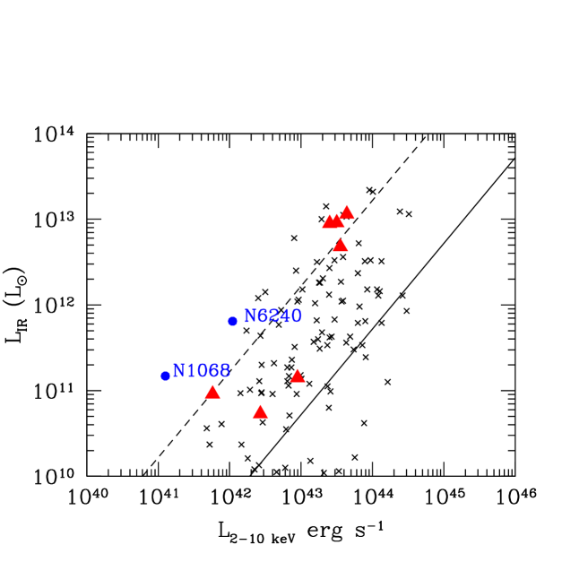
Figure 4: The total IR luminosity against the observed X-ray (2-10 keV) luminosity for the Compton-thick sources (red triangles) and the other X-ray sources (crosses). The solid line corresponds to the average IR to X-ray luminosity expected for an unabsorbed AGN while the dashed line corresponds roughly that expected in the case of a Compton-thick source (see text). The blue circles denote the nearby Compton-thick AGN, NGC1068 and NGC6240.

The ratio of the observed X-ray to IR luminosity can provide further clues on whether a source is obscured. The ratio of the X-ray to the IR luminosity should be suppressed in the most obscured sources (eg Alexander et al. 2005). We present the total IR luminosity against the 2-10 keV absorbed luminosity in Fig. 4. The total IR luminosity is derived using our SED fitting model. Note that four of our candidate Compton-thick sources are outside the area covered by the Spitzer survey. In one case (35), we quote instead the IR luminosity given by Chapman et al. (2005). The solid line denotes the area populated by unabsorbed AGN, while the dashed line indicates the area populated by Compton-thick sources. In the case of Compton-thick sources we assumed that the reflected emission represents 3% of the intrinsic emission (e.g. Comastri 2004, Akylas & Georgantopoulos 2009). Most sources show a low ratio of X-ray to IR luminosity consistent with being Compton-thick. We note that although normal galaxies populate the same space of the X-ray/IR diagram, none of our sources can be associated with such objects. This is because normal galaxies have steep spectra and low X-ray luminosities (e.g. Georgakakis et al. 2006, Tzanavaris & Georgantopoulos 2008 and references therein). At least one source (107) appears to have a high X-ray to IR flux ratio casting doubt on its classification as a Compton-thick source. Intriguingly, this source is an 24$\mu m$ luminous, optically faint source and thus in principle should be an excellent candidate for being obscured (see Fig. 6). Four of our candidate Compton-thick sources have high total IR luminosities ($\rm>10^{12}L_{\odot}$) lying in the Ultraluminous IRAS Galaxy (ULIRG) regime (Sanders & Mirabel 1996). All these are sub-mm luminous galaxies (Chapman et al. 2005, Alexander et al. 2005) at a redshift higher than two.

Table 3: IR properties of the X-ray selected Compton-thick AGN

ID	z	$3.6\mu m$	$4.5\mu m$	$5.8\mu m$	$8.0\mu m$	$24\mu m$	$R-[24]$	$logL_{IR}$	Comments
(1)	(2)	(3)	(4)	(5)	(6)	(7)	(8)	(9)	(10)
35	2.203	-	-	-	-	-	-	$12.95^{\dagger}$	sub-mm, oSFR
91	0.51	-	-	-	-	-	-	-
92	0.91	17.82	17.07	16.64	16.27	160.6	14.16	11.15	irAGN
107	0.59	18.54	17.49	16.47	15.45	325.3	16.1	10.73	irSFR
121	0.520	-	-	-	-	-	-	-	-
127	1.014	-	-	-	-	-	-	-
135	2.466	17.91	17.05	16.31	15.97	376.4	13.88	11.6	sub-mm, oSFR, irSFR
171	1.993	17.86	17.09	15.92	14.38	801.1 7	13.60	12.96	sub-mm, oAGN, irAGN
190	2.005	16.60	15.64	14.53	13.33	1426.0	14.32	13.06	sub-mm, oAGN, irAGN
191	0.276	16.08	15.81	15.55	14.77	-	-	10.96	irSFR

• The columns are: (1) Alexander ID number; (2): redshift ; three and two decimal numbers refer to spectroscopic and photometric redshift respectively; (3) 3.6$\mu m$ flux in units of $\mu Jy$ ; (4) 4.5$\mu m$ flux in units of $\mu Jy$ ; (5) 5.8$\mu m$ flux in units of $\mu Jy$ ; (6) 8.0$\mu m$ flux in units of $\mu Jy$ ; (7) 24$\mu m$ flux in units of $\mu Jy$ ; (8) R-[24] colour (Vega); (9) Logarithm of the total IR luminosity in units of $L\odot$ (10) Comments: sub-mm denotes that the source is a sub-mm galaxy in the sample of Chapman et al. 2005; irAGN or irSFR denotes whether the source has been classified as a star-forming galaxy or an AGN according to the IR-SED fit; oAGN or oSFR denotes that the source has been classified as an AGN or a starburst according to the optical spectrum of Chapman et al. 2005 $\dagger$: Luminosity from Chapman et al. 2005

4 Discussion

4.1 X-ray properties

Our X-ray spectroscopy method revealed 10 candidate Compton-thick sources. Only one is a transmission object while the other 9 are reflection-dominated. The transmission object at a spectroscopic redshift of z=2.466 can be considered as the more robust Compton-thick case as we see the spectral curvature directly. Its column density is $\sim 3\times 10^{24}$ $\rm cm^{-2}\leavevmode\nobreak\$. The most distant reflection-dominated source in our sample is at a redshift of z=2.2. At this redshift the column density should exceed $\sim 5\times 10^{24}$ $\rm cm^{-2}\leavevmode\nobreak\$so that the transmitted emission is not redshifted and thus observable in the Chandra passband. This would be then comparable to the the highest column densities observed in the local Universe (e.g. NGC4945, Itoh et al. 2008).

4.1.1 Fe lines

The presence of high equivalent width $\rm FeK\alpha$ lines should provide conclusive evidence on whether our sources are Compton-thick. High equivalent width $\rm FeK\alpha$ lines are present in the two nearest Compton-thick AGN (NGC1068, Matt et al. 2004; Circinus, Yang et al. 2009). This line is often considered to be the ’smoking gun’ revealing the presence of a heavily obscured nucleus. In our sample, there is no clearcut evidence for the presence of a strong ($>$1 keV) $\rm FeK\alpha$ line which would unambiguously classify a source as a bona-fide Compton-thick AGN. We clearly detect a $\rm FeK\alpha$ line in the case of the source 190 (but with an EW 90% upper limit of only $\sim$700 eV). In three cases we are observing features which are consistent with strong emission lines but not at the 6.4 keV rest-frame energy. As all three sources have only photometric redshift available, it is possible that these features correspond indeed to $\rm FeK\alpha$ lines. The EW in all the above cases present large uncertainties, but interestingly none exceeds 1 keV at the 90% upper limit. In other cases, the derived upper limits are consistent with high EW (e.g. sources 135, 170) while in the case of the sources 35, 92 and 121, the 90% upper limits are low ($<$500 eV).

We have attempted to coadd the spectra in order to put more stringent constraints on the presence of an Fe line. We use only the six objects with spectroscopic redshift available (see table 1). The addition of the ungrouped spectra has been done in the following way. We first obtain for each source the unfolded spectrum, corrected for instrumental effects, using XSPEC. We then shift each bin to the rest-frame energy according to the redshift of each source. At this stage the spectra are stacked. The spectrum is shown in Fig. 5. The data are grouped in 0.5 keV bins. An FeK$\alpha$ line at 6.4 keV rest-frame is clearly detected, with an EW of $790^{+500}_{-650}$ eV.

Figure 5: The stacked X-ray spectrum of the six candidate Compton-thick sources with spectroscopic redshift available.

Next, we discuss whether the absence of strong lines argues against the presence of Compton-thick AGN. Murphy & Yaqoob (2009) present Monte-carlo simulations for Compton-thick reprocessors. For a column density of $10^{24}$ $\rm cm^{-2}\leavevmode\nobreak\$and for a toroidal geometry, they predict EW varying between 100 and 400 eV depending on the viewing angle (but see also the models of Ikeda et al. 2009). The EW rise up to 1 keV for column densities $\rm N_{H}\sim 10^{25}$ $\rm cm^{-2}\leavevmode\nobreak\$. Therefore, the models of Murphy & Yaqoob (2009) would tend to suggest that at least some of our objects are not transmission dominated Compton-thick sources. Nevertheless, it is possible that there is large variety of obscuring screen geometries resulting in a wide range of FeK$\alpha$ line EW. For example, in the SWIFT/BAT sample of Winter et al. (2009) there is a large number of sources with column densities very close to $10^{24}$ $\rm cm^{-2}\leavevmode\nobreak\$. These have EW ranging within an order of magnitude from about 100 to 1000 eV. This clearly demonstrates the uncertainty in determining the column density from the EW of the FeK$\alpha$ line (see also Brightman & Nandra 2008 for the case of IRASF 01475-0740).

4.2 IR, sub-mm and optical properties

Four of our Compton-thick AGN are bright sub-mm sources providing further indirect evidence that these may host heavily buried nuclei. These include the transmission dominated source. Alexander et al. (2005) independently argued that these sources host Compton-thick nuclei. These authors discuss the properties of the common X-ray/sub-mm sources in the CDFN. They find that 11 X-ray sources coincide with sub-mm sources down to the X-ray flux level adopted here i.e. $\rm f_{2-10\leavevmode\nobreak\ keV}=10^{-15}$ $\rm erg\,cm^{-2}\,s^{-1}$ . Good quality optical spectra are available for the four sub-mm sources from Chapman et al. (2005). As discussed by these authors, only two of these show AGN signatures while the other two are consistent with star-forming galaxy spectra. Pope et al. (2008b) and Menendez-Delmestre (2009) present Spitzer IRS spectra of sub-mm galaxies. These include our Compton-thick candidate sources 135 and 35. The IRS spectra of these two sources appear to be dominated by star-forming emission i.e. flat continua, PAH emission features. They also present strong silicate absorption features suggestive of large column densities.

The Spitzer mission revealed a class of bright Infrared, optically faint sources (Houck et al. 2005). These have extreme 24$\mu m$ to R-band flux ratios $\rm f_{24}/f_{R}\sim 1000$ or $R-[24]>14$ (Dey et al. 2008). These are often referred in the literature as Dust Obscured galaxies (DOGs). Fiore et al. (2008) propose that the majority of these sources are associated with Compton-thick sources at high redshift. Our five Compton-thick candidate sources with available Spitzer mid-IR data, have very high mid-IR to optical flux values: $R-[24]>13.6$. In Fig. 6 we give the R-[24] magnitude for our candidate Compton-thick sources in comparison with the rest of our sample. The candidate Compton-thick sources populate the upper (i.e. redder or optically faint) part of the diagram. This provides additional support to the claims which link the infrared bright, optically faint sources (DOGs) with Compton-thick AGN. Pope et al. (2008) assert that the DOG population is substantially contaminated by star-forming galaxies. These authors have proposed a diagnostic diagram for DOGs. In particular they find that the DOGs which are associated with star-forming galaxies, according to Spitzer IRS spectroscopy, have a flux ratio $S_{8.0}/S_{4.5}<2$, while the AGN present higher values. This is not the case in our sample. From table 3, we see that all six candidate Compton-thick AGN with available Spitzer data have $S_{8.0}/S_{4.5}<1$ and thus would be classified as star-forming galaxies according to the above criterion.

It is instructive to examine the location of our candidate Compton-thick sources on the Spitzer IRAC mid-IR colour-colour diagram. Stern et al. (2005) have demonstrated that this diagram provides an efficient diagnostic for AGN identification. In particular, AGN are found to occupy the ’red’ part of the [3.6]-[4.5] vs [5.8]-[8.0] band diagram. The power-law IR spectrum sources of Donley et al. (2007) or Alonso-Herrero et al. (2007) would also fall in this ’wedge’. We plot the colour-colour diagram in Fig.7. From the five candidate Compton-thick sources only three (107, 171, 190) appear to be inside the AGN wedge. One source (191) is lying just below the wedge on a region occupied by normal galaxies (see e.g. Barmby et al. 2006). Finally two more sources (135 and 92) are having [5.8]-[8.0] colours bluer than the AGN. This is the part of the diagram which is populated by the mid-IR bright, optically faint sources (see Georgantopoulos et al. 2008). It appears then that the IR AGN selection methods based on either colours or power-law spectra would fail to detect a large fraction of Compton-thick candidates.

Finally, we examine the relation of our candidate Compton-thick sources with the extreme X-ray to optical flux ratio sources (Koekemoer et al. 2004). These sources are believed to be associated with heavily obscured AGN at high redshift. This is because at high redshift the k-correction shifts the optical wavelengths to the UV making them more prone to dust absorption while in contrast the k-correction shifts the X-ray wavelengths to higher energies which are less obscured. This results in an increase of the X-ray to optical flux ratio for absorbed sources with increasing redshift. Civano et al. (2005) present the X-ray spectral properties of the optically faint hard X-ray sources in the CDFN. They find 63 sources with extreme X-ray to optical flux ratios ($\rm\log(f_{x}/f_{o})>1$). According to Civano et al. (2005), the stacked X-ray spectra of these sources suggest that these are heavily obscured sources. Only three sources coincide with the Compton-thick candidates here (sources 91, 92 and 107) suggesting that the extreme X-ray to optical flux ratio method may not be highly efficient for selecting out Compton-thick sources.

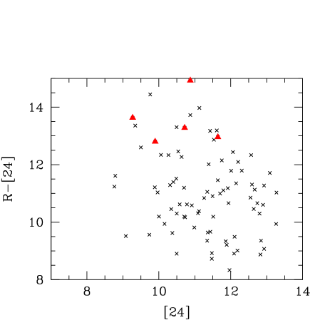
Figure 6: The R-[24] colour vs. [24] magnitude for the 5 candidate Compton-thick sources (red triangles), compared with the other X-ray sources with 24$\mu m$ Spitzer MIPS detections (black crosses).

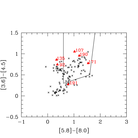
Figure 7: The mid-IR colour-colour diagram for the Compton-thick sources (red triangles) as compared with the other X-ray sources in our sample (black crosses). The ’wedge’ defines the region occupied by mid-IR selected AGN (Stern et al. 2005)

4.3 Comparison with X-ray background synthesis models

Here, we compare the flux distribution as well as the redshift distribution of the 10 candidate Compton-thick AGN with the predictions of the X-ray background synthesis models of Gilli et al. (2007). We use the POMPA code . We assume that Compton-thick AGN have column densities up to $10^{26}$ $\rm cm^{-2}\leavevmode\nobreak\$. The predicted number count distribution logN-logS is given in Fig. 8. If we assumed only sources with column densities $<10^{25}$ $\rm cm^{-2}\leavevmode\nobreak\$, we obtain roughly a factor of two lower normalization in the number counts. Our point agrees well with the logN-logS of Gilli et al. (2007). We also plot the observed number density at bright fluxes derived from the 10 Compton-thick sources of INTEGRAL (Sazonov et al. 2007), as adapted from Treister et al. (2009). The conversion from the 17-60 keV to the 2-10 keV band has been performed assuming a spectrum of $\Gamma\approx 0.2$, i.e. the median spectrum of our sources. Treister et al. (2009) point out that the INTEGRAL number counts are more than a factor of two below the predictions of the Gilli et al. model. This could be partially explained by the fact that the INTEGRAL surveys cannot detect sources with $\rm N_{H}>10^{25}$ $\rm cm^{-2}\leavevmode\nobreak\$, assuming of course that such heavily obscured sources really exist. However, Treister et al. assert that one can obtain a very good fit to the X-ray background spectrum in the 20-40 keV energy range without the need for a large number of heavily obscured sources. This is because of the uncertainties on the normalization of the X-ray background at high energies as well as on the uncertainty on the AGN spectrum at high energy i.e. the normalization of the reflection component.

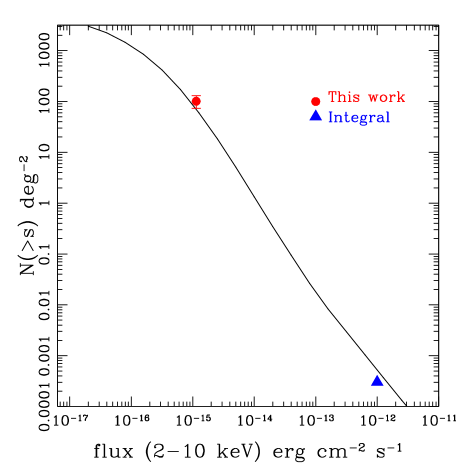
Figure 8: The number counts for the 10 candidate Compton-thick sources (red circle) compared with the predictions (solid line) of the X-ray background synthesis model of Gilli et al. (2007). The blue triangle denotes the INTEGRAL number counts (adapted from Treister et al. 2009). The dash line corresponds to the total logN-logS.

The number count distribution of the Compton-thick population illustrates very well why the Chandra Deep Fields offer the most promising area for detecting Compton-thick AGN, at high redshift, through X-ray spectroscopy. At the flux limit imposed here ($10^{-15}$ $\rm erg\,cm^{-2}\,s^{-1}$ ), we barely accumulate a few hundred photons in order to have a sufficient number of counts for spectral fitting. For a survey with 10 times less exposure time (similar to the COSMOS survey Hasinger et al. 2007; or the AEGIS survey Nandra et al. 2007), we would obtain the same number of photons for sources with a flux of about $10^{-14}$ $\rm erg\,cm^{-2}\,s^{-1}$ . However, the number density at these bright fluxes is only $\rm\sim 1deg^{-2}$ i.e. about two orders of magnitude lower.

Figure 9: The number counts for the 10 candidate Compton-thick sources (triangles) compared with the predictions (solid line) of the X-ray background synthesis model of Gilli et al. (2007)

In Fig. 9 we plot the cumulative redshift distribution for our sample. This is compared with the predictions of the Gilli et al. model. There is rather reasonable overall agreement, given the uncertainties introduced by the photometric redshifts. The number of Compton-thick AGN below a redshift of z=0.5 is about 10% of the total number up to a redshift of z=3. Still these low redshift AGN are the ones which contribute 50% of the X-ray background. Instead the contribution of the high redshift Compton-thick sources is very small: less than 1% for those with $z>2$ (see Treister et al. 2009, Gilli et al. 2007).

5 Conclusions

We have investigated the X-ray spectral properties of the bright CDF-N sources $>10^{-15}$ $\rm erg\,cm^{-2}\,s^{-1}$ selected in the 2-10 keV band. There are 171 sources which have either a spectroscopic or a photometric redshift available. Our aim is to identify Compton-thick candidates either though the presence of a absorption turnover or a reflection-dominated spectrum. Our conclusions can be summarised as follows:

• We find 10 candidate Compton-thick AGN. For six of them there are spectroscopic redshifts while for the remaining only photometric available. One source is a transmission Compton-thick AGN while the other nine are probably reflection dominated.

• We find no high EW ($>1$ keV) FeK$\alpha$ emission line in the individual spectra of our sources. However, the stacked spectrum of the six sources with spectroscopic redshift reveals an FeK$\alpha$ line with an EW of $\approx$800 eV.

• Four sources, including the transmission Compton-thick object, are associated with luminous sub-mm galaxies, at redshift $z\sim 2$ or higher, further supporting the heavily obscured scenario for these.

• For many of the sources with available IR luminosity, we find a low X-ray to total IR luminosity ratio corroborating the presence of obscured accretion.

• Our Compton-thick candidates appear to be associated with optically faint, 24$\mu m$ bright Infrared galaxies in agreement with the findings of Fiore et al. (2008)

• Interestingly, mid-IR selection criteria (e.g. colour-colour diagram) do not appear to be efficient in selecting our candidate Compton-thick AGN. The same applies to methods which use the X-ray to IR or optical flux ratio. Instead, the selection of mid-IR bright and faint optically sources has the most significant overlap with our sample

• The number counts of Compton-thick sources at faint fluxes are in overall agreement with the predictions of the population synthesis models of Gilli et al (2007)

Future observations with the Nustar, Simbol-X and Next missions will provide the first images of the hard X-ray Universe at energies above 10 keV. These are expected to provide a wealth of data on Compton-thick sources at low redshift and place tight constraints on the contribution of these objects to the X-ray background. In the meantime, XMM-Newton can shed light on the properties of Compton-thick sources at moderate to high redshift. The already scheduled 3Ms XMM-Newton observations of the Chandra Deep Field South can provide spectra of unprecedented quality and thus to easily identify the Compton-thick candidate sources.

Appendix A Spectral Simulations

We perform spectral simulations in order to quantify the fraction of Compton-thick candidates that have been erroneously included in our sample. In particular, because of the limited photon statistics, some faint heavily absorbed sources may be mistaken for flat sources. We use XSPEC v.12.4 to create 1000 fake X-ray spectra in the 2-10 keV flux interval of $10^{-14}-10^{-15}$ $\rm erg\,cm^{-2}\,s^{-1}$ i.e. the flux range of the actual Compton-thick sources. The on-axis response and auxilliary files for ${\it Chandra\leavevmode\nobreak\ }$ ACIS-I CCD are used for simplicity. We assume an absorbed power-law model with $\Gamma$ fixed to 1.9 and a column density randomly varying between $10^{20}-10^{24}$ $\rm cm^{-2}\leavevmode\nobreak\$. We fit the fake spectra using XSPEC using an absorbed power-law model with both the $\Gamma$ and $\rm N_{H}$ parameters free. We then estimate the fraction of sources that present a best fit $\Gamma$ value flatter than 1.4 at the 90 per cent upper limit. The spectral fits show that 2 out of 1000 sources are spurious Compton-thick candidates. We note here that these simulated source present high columns ($\rm\sim 6\times 10^{23}$ cm^-2). Our sample contains 141 in the same flux interval. This automatically suggest that the number of the spurious Compton-thick candidates in our sample is $\sim$0.3.

Inversely, it is likely that within the errors, some reflection-dominated flat sources may have a 90% photon index upper limit $\Gamma>1.4$ and thus are missed by our criteria. In order to check this possibility we run another simulation. We create 1000 fake spectra using the PEXRAV model in XSPEC. We assume z=1 and a random 2-10 keV flux between $10^{-15}-10^{-14}$ $\rm erg\,cm^{-2}\,s^{-1}$ . We again fit the spectra in XSPEC using an absorbed power-law model. We estimate the fraction of the sources that show a power-law photon index steeper that 1.4 at the 90 per cent confidence level. Our simulations show that there are no sources with $\Gamma$ less than 1.4 at the 90 per cent upper limit. This immediately suggests that the number of missed Compton-thick sources in our sample is $<0.14$.