Deterministic reaction models with power-law forces

Abstract

We study a one-dimensional particles system, in the overdamped limit, where nearest particles attract with a force inversely proportional to a power $\alpha$ of their distance and coalesce upon encounter. The detailed shape of the distribution function for the gap between neighbouring particles serves to discriminate between different laws of attraction. We develop an exact Fokker-Planck approach for the infinite hierarchy of distribution functions for multiple adjacent gaps and solve it exactly, at the mean-field level, where correlations are ignored. The crucial role of correlations and their effect on the gap distribution function is explored both numerically and analytically. Finally, we analyse a random input of particles, which results in a stationary state where the effect of correlations is largely diminished.

1 Introduction

In a recent paper [1], we have mapped the late-time evolution of the conserved Kuramoto-Sivashinsky (CKS) equation [2],

$$u_{t}=-(u+u_{xx}+u_{x}^{2})_{xx}\,,$$ (1)

used to describe, e.g., the dynamics of meandering steps in crystal growth or that of wind driven sand dunes, to a reacting particles system. The long-time profile $u(x,t)$ is made up of pieces of a universal parabola (solution of the equation $u+u_{xx}+u_{x}^{2}=c$), joining in regions of vanishing size and diverging curvature whose locations define the profile without ambiguity, and that one may associate with ‘particles’. The projected particles on the $x$-axis form an overdamped one-dimensional system; nearest particles attract one another with a force inversely proportional to their distance, and particles coalesce irreversibly upon encounter. This process gives rise to a reduction in the particle density, i.e., to a coarsening process.

In this paper, we generalize the above reaction model to the case where the force between nearest particles, separated by a distance $\ell$, is proportional to $1/\ell^{\alpha}$ ($\alpha=1$ corresponding to the CKS equation). Reacting particles systems such as this, evolving deterministically, occur often enough but have been studied sparingly. Coarsening in spin systems has been studied for exponential forces [3] between the kinks and for power-law forces (between all particle pairs) [4, 5]. The deterministic Kardar-Parisi-Zhang equation corresponds to an interacting particles system [6], and the (non conserved) KS equation was shown to be equivalent to coalescing particles traveling ballistically [7], as is also the case for the Burgers equation at high Reynolds numbers (shocks representing particles) [8]. Similar ballistic systems have been studied by Redner et al. [9]. Simple deterministic reaction schemes, such as the “cut-in-half” model, have been devised by Derrida et al. [10], but exact results are few even in those ideal cases.

The aim of this paper is to give a thorough description of these models with varying $\alpha$. The time-dependence of coarsening can be easily found using dimensional analysis, however, it provides too weak a characterization of the kinetics (e.g., diffusion-limited one-species coalescence coarsens in the same way as our model for $\alpha=1$). We therefore focus on the distribution function $g(\ell,t)$ for the gap $\ell$ between nearest particles. We derive an exact hierarchy of Fokker-Planck equations for the probability density functions (pdf) $\{\rho_{m}\}_{m=1}^{\infty}$, for finding $m$ consecutive gaps of given sizes at time $t$. Truncating this hierarchy at the mean-field level, ignoring correlations between adjacent gaps, we solve for the (approximate) single gap distribution function. The shape of this pdf is a much better discriminant between various models, and we focus in particular on the exponent $\beta$ characterizing the small gap behavior, $g(\ell)\sim\ell^{\beta}$. The role of correlations is explored numerically and analytically, using the Fokker-Planck equations to derive exact constraints that the gap distributions must satisfy when correlations are fully taken into account. Finally, we test the mean-field approximation for the case where a homogeneous random input of particles produces a steady state that is considerably less affected by correlations.

Apart from the intrinsic interest in deterministic reaction models, our particular system might also be relevant to the dynamics of vicinal surfaces undergoing step-bunching instability [11] — a process where parallel straight steps do not move uniformly but rather bunch together in groups separated by large terraces. In this picture, particles represent steps. One of the several ways that steps interact is through diffusion, giving rise to an effective attraction decaying as $1/(b+\ell)$, where $b$ is some characteristic length. For large terraces, the model $\alpha=1$ is recovered, while the opposite limit, $\ell\ll b$, corresponds to our model with $\alpha=-1$.

2 The Model

Consider an infinite system of particles on the line, located at $\{x_{i}(t)\}_{i=-\infty}^{\infty}$. The system is overdamped, and nearest particles attract one another with a force inversely proportional to a power $\alpha$ of the distance:

$$\frac{dx_{i}}{dt}=\frac{A}{\alpha}\left(\frac{1}{(x_{i+1}-x_{i})^{\alpha}}-\frac{1}{(x_{i}-x_{i-1})^{\alpha}}\right)\,.$$ (2)

The prefactor $A$ carries units of $({\rm length})^{\alpha+1}/({\rm time})$ (or ${\rm L}^{\alpha+1}/{\rm T}$, symbolically), and $1/\alpha$ has been introduced to enable discussion of negative $\alpha$, as well as the limit $\alpha\to 0$.

From (2) one finds that the gaps between particles, $\ell_{i}=x_{i+1}-x_{i}$, obey

$$\frac{d\ell_{i}}{dt}=\frac{A}{\alpha}\left(\frac{1}{\ell_{i-1}^{\alpha}}-\frac{2}{\ell_{i}^{\alpha}}+\frac{1}{\ell_{i+1}^{\alpha}}\right)\,.$$ (3)

The particles coalesce upon encounter, or analogously a gap is removed from the system once it has shrunk to zero. Thus, the number of particles decreases and the typical gap between particles grows as the system coarsens with time.

2.1 Linear Stability Analysis

To analyse the system’s stability let us perturb a uniform configuration,

$$\ell_{i}=\left\langle\ell\right\rangle+\epsilon_{i}\,,\qquad\ell_{i}^{-\alpha}\simeq\left\langle\ell\right\rangle^{-\alpha}\left(1-\alpha{\epsilon_{i}\over\left\langle\ell\right\rangle}\right)\,,$$ (4)

and substitute in (3) to yield

$$\dot{\epsilon}_{i}=-{A\over\left\langle\ell\right\rangle^{\alpha+1}}(\epsilon_{i+1}+\epsilon_{i-1}-2\epsilon_{i})\,,$$ (5)

or, upon passing to the continuum limit (for large $i$ and $t$), $\epsilon_{i}\to\epsilon(x,t)$,

$$\frac{\partial}{\partial t}\epsilon(x,t)=-{A\over\left\langle\ell\right\rangle^{\alpha+1}}\frac{\partial^{2}}{\partial x^{2}}\epsilon(x,t)\,.$$ (6)

Thus the perturbations obey a diffusion equation with negative coefficient, and the system is unstable regardless of the sign of $\alpha$: the prefactor $1/\alpha$ introduced in (2) ensures this outcome. For $\alpha>0$ the attractive forces between particles separated by short gaps grow ever stronger, resulting in the eventual coalescence of the particles, and corresponding to singularity buildups in the diffusion equation. For $\alpha<0$, the forces are repulsive and short gaps shrink into singularities due to the dominating forces of the larger surrounding gaps. In the demarcating limit of $\alpha\to 0$ the forces depend logarithmically upon the distance:

$$\frac{dx_{i}}{dt}=A\ln\frac{x_{i}-x_{i-1}}{x_{i+1}-x_{i}}\,;\qquad\frac{d\ell_{i}}{dt}=A\ln\frac{\ell_{i}^{2}}{\ell_{i-1}\ell_{i+1}}\,.$$ (7)

2.2 Simulations

Simulations have been performed by numerical integration of Eq. (2) for systems of $10^{4}$ particles (for $\alpha>0$) and $10^{5}$ particles ($\alpha<0$). The calculations were carried out on a Linux AMD64 cluster comprising 32 processors. Data were obtained by averaging over thousands of independent runs. The long-time asymptotic limit is reached sooner for positive $\alpha$, so typically the runs proceeded until the number of particles dwindled to $500$–$700$ for $\alpha>0$, or $50$–$90$ for $\alpha<0$.

3 Dimensional analysis

Numerical integration of the equations of motion, starting from different initial conditions, suggests that the original state of the system has no effect on its long-time asymptotic behavior. In the long-time regime, therefore, the only dimensional physical parameters determining the typical gap ${\bar{\ell}}$ (a length, L) are the elapsed time $t$ (T) and the constant $A$ (${\rm L}^{\alpha+1}/{\rm T}$), so one expects

$${\bar{\ell}}\sim(At)^{1/(1+\alpha)}\,.$$ (8)

This is indeed confirmed by numerical simulations.

This scaling argument breaks down as $\alpha$ becomes smaller than $-1$. As $\alpha\to-1$ coarsening proceeds ever faster and takes place at a finite time (even in an infinite system) in the limit $\alpha=-1$, and the initial configuration becomes then important. Independence from initial conditions, however, is a prerequisite for the scaling behavior that we assume (and find numerically) in order to analyse the gap distribution in Section 4. Accordingly, we limit the discussion to $\alpha>-1$.

If in addition to the coalescence reaction particles are input randomly, at rate $R$ per unit length per unit time (or $1/{\rm LT}$), the system achieves a steady state that is independent of its initial condition. The typical distance at the steady state is then dependent upon $A$ and $R$ alone, so

$${\bar{\ell}}_{s}\sim\left(\frac{A}{R}\right)^{1/(2+\alpha)}\,.$$ (9)

Physically, the characteristic time for the shrinking of ${\bar{\ell}}_{s}$, ${\bar{\ell}}_{s}^{1+\alpha}/A$, is then balanced by the time $1/{\bar{\ell}}_{s}R$ for getting a new particle into the interval. For the important case of $\alpha=1$, the exponents ${\bar{\ell}}\sim t^{1/2}$ and ${\bar{\ell}}_{s}\sim R^{-1/3}$ agree exactly with the well known cases of diffusion-limited coalescence and diffusion-limited coalescence with input (where the particles diffuse freely without damping and without an attractive force) [12].

4 Gap distributions and Fokker-Planck approach

We see that the coarsening kinetics is not sufficient to distinguish between such different systems as diffusion-limited coalescence, annihilation, and our model with $\alpha=1$. A full characterization of a particles system on the line is provided by the hierarchy of joint pdfs for the multiple-gap correlation functions $\rho_{m}(\ell_{1},\ell_{2},\dots,\ell_{m},t)$ — the probability of finding $m$ consecutive gaps of lengths $\ell_{1},\ell_{2},\dots,\ell_{m}$ at time $t$. This is fully equivalent to the more traditional hierarchy of multiple-point correlation functions $p_{k}(x_{1},x_{2},\dots,x_{k},t)$ for finding $k$ particles at $x_{1},x_{2},\dots,x_{k}$ at time $t$ [13]. In the following, we develop a Fokker-Planck approach for obtaining the $\rho_{m}$. For practical purposes, however, the single gap distribution $\rho_{1}\equiv\rho(\ell,t)$ provides already with enough detail to distinguish between various reaction models. For example, the tail of the distribution falls off as a gaussian, $\rho\sim\exp(-c_{1}\ell^{2}/t)$, for diffusion-limited coalescence, but as a stretched exponential, $\exp(-c_{2}\ell^{3/2})$, for coalescence with input, while for small $\ell$ one finds $\rho\sim\ell^{\beta}$ with $\beta=1$ in both these cases but $\beta\approx 1.3$ for our model with $\alpha=1$. For other values of $\alpha$ one finds that $\beta$ has a non trivial dependence upon $\alpha$ (Fig. 1).

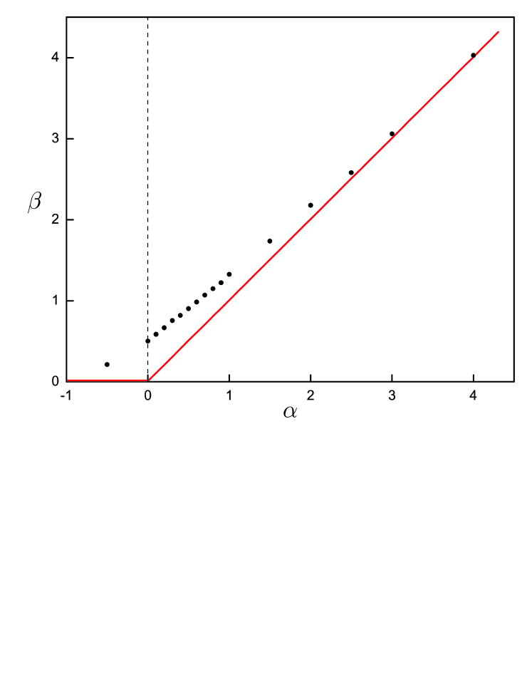
Figure 1: The exponent $\beta$, that describes the small gap behavior of the gap distribution function, $\rho(\ell,t)\sim\ell^{\beta}$, as a function of the force exponent $\alpha$ in our deterministic reaction model. The solid line indicates the mean-field prediction of Eq. (23), $\beta=\alpha$.

Let $n_{m}(\ell_{1},\ell_{2},\dots,\ell_{m},t)d\ell_{1}d\ell_{2}\cdots d\ell_{m}$ denote the number of $m$ consecutive gaps of lengths between $\ell_{j}$ and $\ell_{j}+d\ell_{j}$ ($j=1,2,\dots,m$), at time $t$. $m=1$ corresponds to the single gap distribution $n_{1}d\ell\equiv n(\ell,t)d\ell$ — the number of gaps between length $\ell$ and $\ell+d\ell$, at time $t$. The total number of gaps (or particles),

$$N(t)=\int_{0}^{\infty}n(\ell,t)\,d\ell\sim 1/{\bar{\ell}}\sim t^{-1/(1+\alpha)}\,,$$ (10)

decreases with time, since the total length of the system $\Lambda\sim N(t){\bar{\ell}}$ is constant. Likewise, the normalization for $m>1$ is

$$\int_{0}^{\infty}\cdots\int_{0}^{\infty}n_{m}(\ell_{1},\dots,\ell_{m},t)\,d\ell_{1}\cdots d\ell_{m}=N(t)\,,$$ (11)

assuming periodic boundary conditions. For free boundary conditions the result is $N(t)-m+1$, but $(m-1)$ can be neglected in the thermodynamic limit of $N(0)\to\infty$. The joint probability density, $\rho_{m}$, is related to $n_{m}$ via the $N(t)$ normalization:

$$\rho_{m}(\ell_{1},\dots,\ell_{m},t)=N(t)^{-1}n_{m}(\ell_{1},\dots,\ell_{m},t)\,.$$ (12)

$n_{m}$ experiences a systematic drift, due to the probability “current” ${\bf J}$; $J_{j}=n_{m}v(\ell_{j-1},\ell_{j},\ell_{j+1})$, arising from the deterministic evolution of each of the gaps $\ell_{j}$ at the rate of $d\ell_{j}/dt=v(\ell_{j-1},\ell_{j},\ell_{j+1})=(1/2\alpha)(1/\ell_{j-1}^{\alpha}-2/\ell_{j}^{\alpha}+1/\ell_{j+1}^{\alpha})$, as given by Eq. (3) and absorbing a factor of $2A$ in $t$. Then, using the notation $\vec{\ell}_{m}\equiv(\ell_{1},\dots,\ell_{m})$, we can write the Fokker-Planck equation

$$\frac{\partial}{\partial t}n_{m}(\vec{\ell}_{m},t)=-\sum_{j=2}^{m-1}\frac{\partial}{\partial\ell_{j}}\left[v(\ell_{j-1},\ell_{j},\ell_{j+1})n_{m}(\vec{\ell}_{m},t)\right]$$

$$\hbox to0.0pt{\hss${}-{}$}\frac{\partial}{\partial\ell_{1}}\int_{0}^{\infty}v(\ell^{\prime},\ell_{1},\ell_{2})n_{m+1}(\ell^{\prime},\vec{\ell}_{m},t)\,d\ell^{\prime}$$

$$\hbox to0.0pt{\hss${}-{}$}\frac{\partial}{\partial\ell_{m}}\int_{0}^{\infty}v(\ell_{m-1},\ell_{m},\ell^{\prime\prime})n_{m+1}(\vec{\ell}_{m},\ell^{\prime\prime},t)\,d\ell^{\prime\prime}$$

$$\hbox to0.0pt{\hss${}-{}$}\sum_{j=1}^{m-1}\lim_{\ell_{j}^{\prime}\to 0}\left[v(\ell_{j},\ell^{\prime}_{j},\ell_{j+1})n_{m+1}(\ell_{1},\dots,\ell_{j},\ell_{j}^{\prime},\ell_{j+1},\dots,\ell_{m},t)\right]\,.$$ (13)

Note that since the expression for $d\ell/dt$ requires knowledge of the gaps lengths to the left and right of $\ell$, the drift for $\ell_{1}$ (the second term on the rhs) forces us to consider ${m+1}$ gaps, including $\ell^{\prime}$ (the neighbour of $\ell_{1}$ to its left), and similarly for $\ell_{m}$ (the third term on the rhs) which requires the gap $\ell^{\prime\prime}$ to its right. The last term denotes the creation of $n_{m}$ when the gap $\ell_{j}^{\prime}$ shrinks and disappears (due to coalescence) from the $(m+1)$-gap configuration $\ell_{1},\ell_{2},\dots,\ell_{j},\ell_{j}^{\prime},\ell_{j+1},\dots,\ell_{m}$. Thus the Fokker-Planck equation for $n_{m}$ requires $n_{m+1}$, resulting in an infinite hierarchy of equations.

4.1 Scaling

A useful simplification that gets rid of the time variable $t$ results from the scaling assumption

$$n_{m}(\ell_{1},\dots,\ell_{m},t)=N(t)\rho_{m}(\ell_{1},\dots,\ell_{m},t)=N(t){\bar{\ell}}^{-m}h_{m}(z_{1},\dots,z_{m});\quad z_{j}\equiv\ell_{j}/{\bar{\ell}}\,.$$ (14)

In [1] we have presented simulation results supporting this scaling form for $m=1$, or the single-gap pdf. For $m=2$ we can test the scaling hypothesis in a roundabout way, by focusing on the distribution function of the particles’ speeds

$$p(v,t)=\int_{0}^{\infty}\int_{0}^{\infty}\delta\left(v-|{\textstyle\frac{1}{\alpha}}(\ell^{\prime-\alpha}-\ell^{\prime\prime-\alpha})|\right)\rho_{2}(\ell^{\prime},\ell^{\prime\prime},t)\,d\ell^{\prime}d\ell^{\prime\prime}\,.$$ (15)

A simple change of variables now shows that (14) implies the scaling of the speed pdf: $p(v,t)={\bar{\ell}}^{\alpha}p(v{\bar{\ell}}^{\alpha})$. In Fig. 2 we confirm that this scaling indeed holds, for the case of $\alpha=1$, giving us some confidence in the postulated scaling form (14) for general $m$.

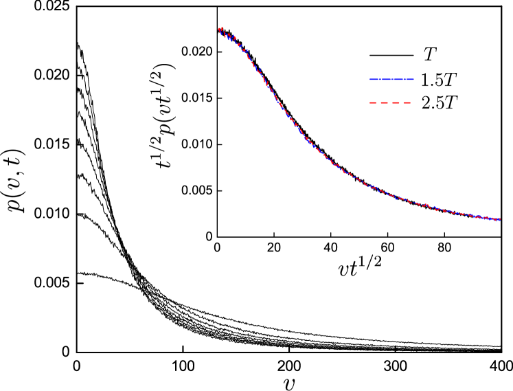
Figure 2: Speed distribution function, shown for several times, for the case of $\alpha=1$. Inset: Collapse of the pdfs is shown for three different times after the scaling regime set in (by time $T$ the initial number of particles has been reduced by a factor of 37), using the relation ${\bar{\ell}}\sim t^{1/2}$, valid for $\alpha=1$.

Using (14) and the fact that $N(t)\sim 1/{\bar{\ell}}$, the Fokker-Planck equation reads,

$$\alpha(m+1)h_{m}(z_{1},\dots,z_{m})+\alpha\sum_{j=1}^{m}z_{j}\frac{\partial}{\partial z_{j}}h_{m}(z_{1},\dots,z_{m})$$ (16)

$$\hbox to0.0pt{\hss${}={}$}\sum_{j=2}^{m-1}\frac{\partial}{\partial z_{j}}\left[\left(\frac{1/2}{z_{j-1}^{\alpha}}-\frac{1}{z_{j}^{\alpha}}+\frac{1/2}{z_{j+1}^{\alpha}}\right)h_{m}(z_{1},\dots,z_{m})\right]$$

$$+\frac{\partial}{\partial z_{1}}\int_{0}^{\infty}\left(\frac{1/2}{z^{\prime\alpha}}-\frac{1}{z_{1}^{\alpha}}+\frac{1/2}{z_{2}^{\alpha}}\right)h_{m+1}(z^{\prime},z_{1},z_{2}\dots,z_{m})\,dz^{\prime}$$

$$+\frac{\partial}{\partial z_{m}}\int_{0}^{\infty}\left(\frac{1/2}{z_{m-1}^{\alpha}}-\frac{1}{z_{m}^{\alpha}}+\frac{1/2}{z^{\prime\prime\alpha}}\right)h_{m+1}(z_{1},\dots,z_{m-1},z_{m},z^{\prime\prime})\,dz^{\prime\prime}$$

$$+\sum_{j=1}^{m-1}\lim_{z_{j}^{\prime}\to 0}\left[\left(\frac{1/2}{z_{j}^{\alpha}}-\frac{1}{z_{j}^{\prime\alpha}}+\frac{1/2}{z_{j+1}^{\alpha}}\right)h_{m+1}(z_{1},\dots,z_{j},z_{j}^{\prime},z_{j+1},\dots,z_{m})\right].$$

In fact, to arrive at this equation it is necessary to assume that ${\dot{\bar{\ell}}}{\bar{\ell}}^{\alpha}$ is a constant (that can be absorbed in the time units, so we take it to be 1). This condition is in agreement with the coarsening law found from dimensional analysis, Eq. (8).

4.2 Truncation scheme and Mean Field solution

Eq. (16) is valid for $m\geq 2$. This infinite hierarchy of equations can be truncated at any level $m$ by the usual Kirkwood approximation scheme:

$$h_{m+1}(z_{1},\dots,z_{m+1})=\frac{h_{m}(z_{1},\dots,z_{m})h_{m}(z_{2},\dots,z_{m+1})}{h_{m-1}(z_{2},\dots,z_{m})}\,.$$ (17)

For example, at the lowest level of $m=2$ we can truncate the hierarchy (16) using

$$h_{3}(z_{1},z_{2},z_{3},)\approx\frac{h_{2}(z_{1},z_{2})h_{2}(z_{2},z_{3})}{h(z_{2})}\,.$$ (18)

This yields

$$3\alpha h_{2}(z_{1},z_{2})+\alpha z_{1}\frac{\partial}{\partial z_{1}}h_{2}(z_{1},z_{2})+\alpha z_{2}\frac{\partial}{\partial z_{2}}h_{2}(z_{1},z_{2})$$

$$\hbox to0.0pt{\hss${}={}$}\frac{\partial}{\partial z_{1}}\left\{h_{2}(z_{1},z_{2})\left[\frac{1/2}{h(z_{1})}\int_{0}^{\infty}\frac{dz^{\prime}}{z^{\prime\alpha}}h_{2}(z_{1},z^{\prime})+\left(\frac{1/2}{z_{2}^{\alpha}}-\frac{1}{z_{1}^{\alpha}}\right)\right]\right\}$$

$$+\frac{\partial}{\partial z_{2}}\left\{h_{2}(z_{1},z_{2})\left[\frac{1/2}{h(z_{2})}\int_{0}^{\infty}\frac{dz^{\prime}}{z^{\prime\alpha}}h_{2}(z_{2},z^{\prime})+\left(\frac{1/2}{z_{1}^{\alpha}}-\frac{1}{z_{2}^{\alpha}}\right)\right]\right\}$$

$$+\lim_{z^{\prime}\to 0}\frac{h_{2}(z_{1},z^{\prime})h_{2}(z_{2},z^{\prime})}{h(z^{\prime})}\left(\frac{1/2}{z_{1}^{\alpha}}-\frac{1}{z^{\prime\alpha}}+\frac{1/2}{z_{2}^{\alpha}}\right)\,,$$ (19)

which is a closed equation for $h_{2}$, since $h(z)\equiv h_{1}(z)=\int_{0}^{\infty}h_{2}(z,z^{\prime})\,dz^{\prime}$. This equation is hard to solve, or even to work out its limiting behavior. We simplify further by making the mean-field assumption that adjacent gaps are not correlated, so that

$$h_{2}(z_{1},z_{2})=h(z_{1})h(z_{2})\,.$$ (20)

Inserting this in (4.2) and integrating over $z_{2}$, we obtain

$$2\alpha h(z)+\alpha zh^{\prime}(z)=\left[\left(\left\langle\frac{1}{z^{\alpha}}\right\rangle-\frac{1}{z^{\alpha}}\right)h(z)\right]^{\prime}\,,$$ (21)

where the prime denotes differentiation with respect to $z$. Thus,

$$\frac{h(z)^{\prime}}{h(z)}=\frac{-2\alpha+\alpha z^{-\alpha-1}}{\alpha z+z^{-\alpha}-\left\langle z^{-\alpha}\right\rangle}\,.$$ (22)

A naive inspection of Eq. (22) in the limit of large $z$ leads to the erroneous conclusion that $h(z)\sim 1/z^{2}$. The problem is with $\left\langle z^{-\alpha}\right\rangle$ (which must be determined self-consistently): depending on its value, the denominator on the rhs might vanish, yielding a singularity that must be taken into account. Proceeding more carefully, we multiply Eq. (21) by $z^{k}$ and integrate over $z$, from $0$ to $\infty$, to yield

$$2\alpha\left\langle z^{k}\right\rangle+\alpha z^{k+1}h(z)|_{z=0}^{\infty}-\alpha(k+1)\left\langle z^{k}\right\rangle$$

$$\hbox to0.0pt{\hss${}={}$}[z^{k}(\left\langle z^{-\alpha}\right\rangle-z^{-\alpha})h(z)]_{z=0}^{\infty}-k\left\langle z^{-\alpha}\right\rangle\left\langle z^{k-1}\right\rangle+k\left\langle z^{k-1-\alpha}\right\rangle\,.$$

Putting $k=0$ we obtain the small-$z$ behavior of $h(z)$:

$$h(z)\longrightarrow\cases{\alpha z^{\alpha}&for $\alpha>0$,\\ |\alpha|/\left\langle z^{|\alpha|}\right\rangle&for $\alpha<0$.}$$ (23)

For $k\to\infty$, and assuming that $h(z)$ has finite support so that the various moments exist and $\lim_{k\to\infty}\left\langle z^{k+c}\right\rangle/\left\langle z^{k}\right\rangle=1$, we get, for the unknown ($-\alpha$)-moment,

$$\left\langle z^{-\alpha}\right\rangle=1+\alpha\,.$$ (24)

Armed with this information we now examine the denominator on the rhs of (22): For $\alpha>0$, $\alpha z+z^{-\alpha}$ achieves a minimum of $1+\alpha$, at $z=z_{c}=1$, so that the denominator is always positive except at $z=z_{c}$, where it vanishes. Meanwhile, the numerator, $-2\alpha+\alpha z^{-\alpha-1}$ is positive at $z<z_{m}=(1/2)^{1/(1+\alpha)}$, and negative for $z>z_{m}$, (note $z_{m}<z_{c}$). Therefore, $h(z)$ rises as $\alpha z^{\alpha}$ (for $z$ near $0$), reaching a maximum at $z=z_{m}$, then drops back to zero as $z$ approaches $z_{c}$. The finite support assumed a priori is caused by the singularity at $z_{c}$ and is now seen to be justified. For $\alpha<0$ (but $\alpha>-1$), $\alpha z+z^{-\alpha}$ achieves a maximum of $1+\alpha$, at $z=z_{c}=1$, so that the denominator is always negative except at $z=z_{c}$, where it vanishes. The numerator is negative for $z<z_{m}$ and positive for $z>z_{m}$, so $h(z)$ starts at $|\alpha|/(1-|\alpha|)$ at $z=0$, rising to a maximum at $z=z_{m}$ and drops back to zero towards $z=z_{c}=1$.

For the case of $\alpha<0$ one can derive from (22) the correction to $h(0)$:

$$h(z)\approx h(0)\left(1+\frac{z^{|\alpha|}}{\left\langle z^{|\alpha|}\right\rangle}\right)=\frac{|\alpha|}{1-|\alpha|}\left(1+\frac{1}{1-|\alpha|}z^{|\alpha|}\right)\,,\qquad\alpha<0\,,$$ (25)

where we have used (23) and (24) for the last equality. Numerically, it is impossible to separate between the finite $h(0)$ and the non-analytic correction, as both result in an infinite slope as $z\to 0$. Indeed, the exponent $\beta$ measured for $\alpha=-1/2$ in Fig. 1 was obtained assuming $h(0)=0$, yielding only an effective value.

Finally, it is possible to obtain explicit solutions for several values of $\alpha$. For example, for the special cases of $\alpha=1,2$, and $-1/2$ we get

$$h(z)=\frac{z}{(1-z)^{3}}\,e^{-z/(1-z)}\,,\qquad 0\leq z\leq 1\,;\qquad\alpha=1\,,$$ (26)

$$h(z)=\frac{2z^{2}}{(1-z)^{26/9}(1+2z)^{10/9}}\,e^{-\frac{2}{3}z/(1-z)}\,,\qquad 0\leq z\leq 1\,;\qquad\alpha=2\,,$$ (27)

$$h(z)=\frac{1}{(1-\sqrt{z})^{4}}\,e^{-2\sqrt{z}/(1-\sqrt{z})}\,,\qquad 0\leq z\leq 1\,;\qquad\alpha=-1/2\,.$$ (28)

In all these cases (and others) it is easy to confirm the predicted small $z$ behaviour, the location of the maximum at $z_{m}=(1/2)^{1/(1+\alpha)}$, the finite support to $z<z_{c}=1$, and that indeed $\left\langle z^{-\alpha}\right\rangle=1+\alpha$. In Figs. 3 and 4 we compare these mean-field results to numerical simulations. Fig. 4 additionally demonstrates that the scaling regime is achieved, numerically, also for $\alpha<0$, though this takes a lot longer than for $\alpha>0$. Reaching scaling from an initial random configuration proved impractical and we had to start the system with all the gaps nearly equal but for tiny perturbations.

For $\alpha\gg 1$ the forces on particles across narrow gaps is immense and unaffected by neighbouring particles, therefore one expects that the mean-field prediction for small gaps improves as $\alpha$ increases (notice indeed the increasing agreement in $\beta$ as $\alpha\to\infty$, in Fig. 1). For $\alpha<0$, on the other hand, it is the force across unusually large gaps that dominates and is unaffected by neighbouring particles, so there we expect that mean-field predicts the tail of the distribution increasingly better as $\alpha$ approaches $-1$.

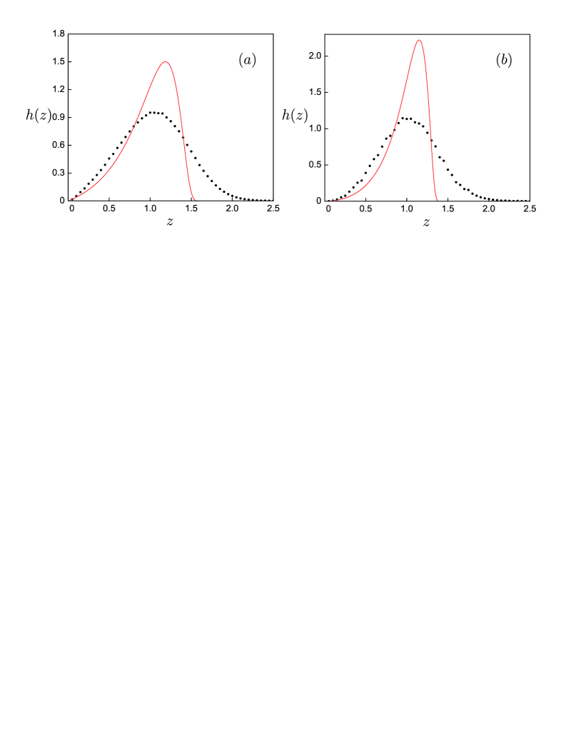
Figure 3: Comparison of $h(z)$ from Eqs. (26), (27) (solid curves) to actual simulations (symbols), for the cases of $\alpha=1$ (a) and $\alpha=2$ (b). In both cases $z$ has been rescaled so that $\left\langle z\right\rangle=1$.

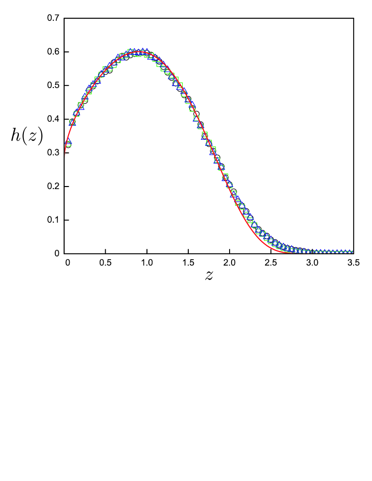
Figure 4: Gap distribution for $\alpha=-1/2$. Simulations are shown for times $T$ (triangles), $1.5T$ (squares), and $2.5T$ (circles) after the scaling regime had been reached: by time $T$ the particles had been decimated 667-fold. The solid curve represents the mean-field result from Eq. (28). For the sake of comparison, $z$ has been rescaled to yield $\left\langle z\right\rangle=1$.

5 The Role of Correlations

Consider now correlations between adjacent gaps $\ell$ and $\ell^{\prime}$. We expect that the two gaps are strongly anti-correlated: as the particle separating the two gaps moves one gap grows on expense of the other. This anti-correlation is clearly visible in Fig. 5, where we compare the (unconstrained) gap distribution to the gap distribution of $\ell$ when $\ell^{\prime}<0.5\left\langle\ell\right\rangle$ and when $\ell^{\prime}>1.5\left\langle\ell\right\rangle$, for the case of $\alpha=1$.

Despite the intractable equation for $h_{2}$ it is possible to make a precise statement on the effect of correlations. We start with the exact equation

$$\frac{\partial}{\partial t}n(\ell,t)=-\frac{\partial}{\partial\ell}\int_{0}^{\infty}\int_{0}^{\infty}v(\ell^{\prime},\ell,\ell^{\prime\prime})n_{3}(\ell^{\prime},\ell,\ell^{\prime\prime},t)\,d\ell^{\prime}d\ell^{\prime\prime}\,,$$ (29)

and use the scaling hypothesis (14) to yield

$$2\alpha h(z)+\alpha z\frac{\partial}{\partial z}h(z)=\frac{\partial}{\partial z}\int_{0}^{\infty}\frac{dz_{1}}{z_{1}^{\alpha}}h_{2}(z,z_{1})-\frac{\partial}{\partial z}\frac{h(z)}{z^{\alpha}}\,.$$ (30)

Integrating over $z$ we get

$$\alpha=\left[h(z)\left\langle{1\over z_{1}^{\alpha}}\right\rangle_{z}-{h(z)\over z^{\alpha}}\right]^{z=\infty}_{z=0},$$ (31)

where we have used the notation

$$\left\langle{1\over z_{1}^{\alpha}}\right\rangle_{z}=\int_{0}^{\infty}{dz_{1}\over z_{1}^{\alpha}}{h_{2}(z,z_{1})\over h(z)}\,,$$

for the conditional average of $z_{1}^{-\alpha}$ subject to the constraint that the interval $\ell_{1}=z_{1}{\bar{\ell}}$ is adjacent to an interval of length $\ell=z{\bar{\ell}}$. It is also understood that the limit of $z\to\infty$ needs changing to $z\to z_{c}$ if there is finite support.

Suppose that $\alpha>0$. It is easy to realise that the first term does not contribute for $z=0$ and the second term does not contribute for $z=\infty$. Therefore, we get

$$\alpha=\lim_{z\to\infty}h(z)\left\langle{1\over z_{1}^{\alpha}}\right\rangle_{z}+\lim_{z\to 0}{h(z)\over z^{\alpha}}.$$ (32)

If one neglects correlations the term $\left\langle z_{1}^{-\alpha}\right\rangle_{z}$ does not depend on $z$, $h(z)$ vanishes for large $z$, and we found $h(z)\sim\alpha z^{\alpha}$ for small $z$, which agrees with Eq. (23).

If we take correlations into account, we know from simulations that $h(z)\sim z^{\beta}$, with $\beta>\alpha$ (Fig. 1), and the second term vanishes. Therefore, $\left\langle z_{1}^{-\alpha}\right\rangle_{z}$ must diverge as $1/h(z)$ as $z\to\infty$. Such behavior is believable, in view of Fig. 5, where we see that the conditional gap distribution when the adjacent gap is unusually large changes the $\beta$ exponent for the small-$z$ behavior. The change in $\beta$ could result in divergence of the $(-\alpha)$-moment in the required way.

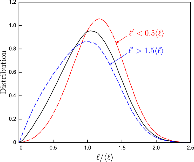
Figure 5: Anti-correlation between adjacent gaps $\ell$ and $\ell^{\prime}$ (for $\alpha=1$). The unconstrained gap distribution of $\ell$ (solid line) is compared to the gap distribution when the adjacent gap $\ell^{\prime}$ is unusually large, $\ell^{\prime}>1.5\left\langle\ell\right\rangle$, and unusually narrow, $\ell^{\prime}<0.5\left\langle\ell\right\rangle$.

The following simple example serves to illustrate how such behavior may arise from anti-correlations. Suppose that two adjacent gaps, $x$ and $y$, are perfectly anti-correlated, such that their sum is fixed:

$$h_{2}(x,y)\sim x(2-x)\delta(x+y-2)\,,\qquad 0\leq x,y\leq 2\,,$$

the $\delta$-function ensuring that $x+y=2$. Integrating over $x$ we get $h(y)\sim y(2-y)$ (note that the example is symmetric; a similar $h(x)$ is obtained integrating over $y$). Therefore,

$$\left\langle\frac{1}{x}\right\rangle_{y}=\int_{0}^{2}\frac{1}{x}\frac{h(x,y)}{h(y)}\,dx=\int_{0}^{2}\frac{1}{x}\frac{x(2-x)}{y(2-y)}\delta(x+y-2)\,dx=\frac{1}{2-y}\,,$$

which diverges in the same way as $1/h(y)$, as $y$ approaches the upper support limit of $y_{c}=2$.

Let us now analise Eq. (31) for negative $\alpha$. The terms evaluated at $z=\infty$ (or $z=z_{c}$) vanish and the term $h(z)z^{|\alpha|}$ vanishes at $z=0$ as well. Therefore, we have

$$h(0)\lim_{z\to 0}\left\langle z_{1}^{|\alpha|}\right\rangle_{z}=|\alpha|=h_{\hbox{\tiny MF}}(0)\left\langle z_{1}^{|\alpha|}\right\rangle_{\hbox{\tiny MF}}\,,$$ (33)

where we have used Eq. (23) for the last equality. Thus, for $\alpha<0$, correlations revise the value of $h(0)$.

5.1 Input

For homogeneous random input at rate $R$, we must add to the rhs of Eq. (29) the terms

$$R\left(-\ell\,n(\ell,t)+2\int_{\ell}^{\infty}n(\ell^{\prime},t)\,d\ell^{\prime}\right)\,.$$

The first term accounts for losses of a gap of length $\ell$, which are proportional to $R\ell$ and to the probability for having the gap in the first place, while the second term accounts for the creation of gaps when a particle is deposited inside a gap $\ell^{\prime}>\ell$, exactly at distance $\ell$ from either edge. Because of the randomizing effect of the input we expect that correlations play a lesser role and the mean-field approximation does somewhat better in this case.

We specialize to the steady-state, setting the time derivative to zero, and use the mean-field ansatz to obtain

$$0=-\frac{1}{\alpha}\frac{\partial}{\partial z}\left[\left(\left\langle\frac{1}{z^{\alpha}}\right\rangle-\frac{1}{z^{\alpha}}\right)h(z)\right]-zh(z)+2\int_{z}^{\infty}h(z^{\prime})\,dz^{\prime}\,,$$ (34)

where now $z=\ell/\ell_{s}$, ($\ell_{s}\sim(A/R)^{1/(2+\alpha)}$). The small-$z$ behaviour is very similar to that without input; $h(z)\sim\alpha\left\langle z\right\rangle z^{\alpha}$ for $\alpha>0$, and $h(z)\sim h(0)(1+z^{|\alpha|}/\left\langle z^{|\alpha|}\right\rangle)$, $h(0)=|\alpha|\left\langle z\right\rangle/\left\langle z^{|\alpha|}\right\rangle$, for $a<0$, while for large $z$ mean-field predicts $h(z)\sim\exp(-c_{1}z^{2})$ for $\alpha>0$, and $h(z)\sim\exp(-c_{2}z^{2-|\alpha|})$ for $\alpha<0$ ($c_{1}=\alpha$ and $c_{2}=|\alpha|/(2-|\alpha|)$ are constants). These predictions seem to be borne out by simulations, although it is hard to make firm statements for the large-$z$ tail. The large-$z$ tail of the distribution for $\alpha=1$ provides yet another difference from diffusion-limited coalescence, where in the case of input $p(z)\sim\exp(-cz^{3/2})$ [12].

In Fig. 6 we compare simulations and numerical integration of the mean-field equation for several values of $\alpha$. The results are quite impressive, suggesting that input kills correlations very effectively.

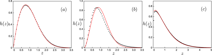
Figure 6: Gap distributions for (a) $\alpha=1$, (b) $\alpha=2$, and (c) $\alpha=-1/2$ in the case of input. Simulations (symbols) are compared to numerical integration of the mean-field equation (34). In all cases $z$ has been rescaled to yield $\left\langle z\right\rangle=1$.

6 Summary and Discussion

In summary, we have analysed a class of deterministic reactions where nearest particles attract as $1/\ell^{\alpha}$ and coalesce upon encounter. The coarsening law is not sufficient to distinguish between different reaction dynamics so we have focused instead on the distribution function $\rho(\ell,t)$ for the gap $\ell$ between nearest particles. We have developed an exact Fokker-Planck hierarchy of equations for the probabilities $\rho_{m}$ for finding $m$ adjacent gaps of given sizes, capitalizing on the fact that the $\rho_{m}$ provide a complete description of a one-dimensional particles system. Truncating the hierarchy at the lowest level, we have studied the gap distribution at the mean-field approximation, neglecting all correlations between adjacent gaps. While this provides a qualitative description of the gap distribution, important details, such as the $\beta$ exponent describing the small gap behavior $\rho(\ell,t)\sim\ell^{\beta}$, could not be captured in this way. The role of correlations, however, was fully elucidated and we have found exact constraints that the distribution functions ought to obey due to their effect. The mean-field approximation worked more satisfactorily for the case of random input, where the role of correlations is diminished, yielding the same $\beta$ exponent observed in simulations.

Perhaps the largest outstanding problem is how to proceed, analytically, beyond the lowest mean-field truncation level, to obtain a more satisfying description of the gap distribution function and of the exponent $\beta$. Especially intriguing is the numerical result that $\beta\approx 1/2$ for $\alpha=0$: Could this be derived exactly, maybe by a totally different approach? Cracking that question could suggest a more direct way of estimating $\beta$ for all $\alpha$ values and perhaps for other deterministic reaction schemes.

References

References

[1]
P. Politi and D. ben-Avraham,
Physica D 238, 156 (2009).
[2]
Z. Csahok, C. Misbah, F. Rioual, A. Valance,
Eur. Phys. J. E 3, 71 (2000);
F. Gillet, Z. Csahok, C. Misbah,
Phys. Rev. B 63, 241401 (2001);
T. Frisch, A. Verga,
Phys. Rev. Lett. 96, 166104 (2006).
[3]
K. Kawasaki, M. C. Yalabik, and J. D. Gunton,
Phys. Rev. B 17, 455 (1978);
T. Ohta, D. Jasnow, and K. Kawasaki,
Phys. Rev. Lett. 49, 1223 (1982).
[4]
I. Ispolatov and P. L. Krapivsky,
Phys. Rev. E 53, 3154 (1996).
[5]
A. D. Rutenberg and A. J. Bray,
Phys. Rev. E 50, 1900 (1994).
[6]
E. Medina, T. Hwa, M. Kardar, Y.-C. Zhang,
Phys. Rev. A 39, 3053 (1989).
[7]
M. Rost and J. Krug,
Physica D 88, 1 (1995).
[8]
J. M. Burgers, The nonlinear diffusion equation
(Riedel, Boston, 1974).
[9]
See, for example, S. Redner,
in Nonequilibrium Statistical Mechanics in One Dimension, V. Privman, ed., (Cambridge University Press, 1997), and references therein.
[10]
B. Derrida, Godreche, and Yekutieli,
Phys. Rev. A 44, 6241 (1991).
[11]
J. Krug, V. Tonchev, S. Stoyanov, and A. Pimpinelli,
Phys. Rev. B 71, 045412 (2005).
[12]
D. ben-Avraham, M. A. Burschka, and C. R. Doering,
J. Stat. Phys. 60, 695 (1990).
[13]
E. Brunet and D. ben-Avraham, J. Phys. A 38, 3247 (2005).