Improved estimate of electron capture rates on nuclei during stellar core collapse

Abstract

Electron captures on nuclei play an important role in the dynamics of the collapsing core of a massive star that leads to a supernova explosion. Recent calculations of these capture rates were based on microscopic models which account for relevant degrees of freedom. Due to computational restrictions such calculations were limited to a modest number of nuclei, mainly in the mass range $A=45$–$110$. Recent supernova simulations show that this pool of nuclei, however, omits the very neutron-rich and heavy nuclei which dominate the nuclear composition during the last phase of the collapse before neutrino trapping. Assuming that the composition is given by Nuclear Statistical Equilibrium we present here electron capture rates for collapse conditions derived from individual rates for roughly $2700$ individual nuclei. For those nuclei which dominate in the early stage of the collapse, the individual rates are derived within the framework of microscopic models, while for the nuclei which dominate at high densities we have derived the rates based on the Random Phase Approximation with a global parametrization of the single particle occupation numbers. In addition, we have improved previous rate evaluations by properly including screening corrections to the reaction rates into account.

1 Introduction

Near the end of their lives, the core of a massive star ($M\geq 10M_{\odot}$) consists predominantly of iron and its nuclear neighbors, the “iron group” elements. Since nuclear burning processes continue in the layers above, this iron core grows, approaching the Chandrasekhar mass limit, and begins contracting at an ever increasing rate. In the inner regions of the core, this collapse is subsonic and homologous, while the outer regions collapse supersonically. With densities larger than $10^{9}$ g/cm³, both transport of electromagnetic radiation and heat conduction are very slow compared with the time-scale of the collapse. The majority of the energy is transported away from the core by neutrinos, originating mostly from electron captures on protons and nuclei [1]. Escaping neutrinos reduce the entropy of the core, forcing nucleons to remain as part of nuclei, until the neutrinos become trapped at densities $10^{11}$–$10^{12}$ g/cm³. $\beta^{-}$-decay processes are effectively blocked by the electron degeneracy, causing nuclei in the core to become progressively more neutron-rich.

Once the density in the innermost part of the collapsing star exceeds that of nuclear matter, the collapse is halted by the short-range repulsion of the nuclear interaction. The supersonically infalling matter of the outer core bounces off this extremely stiff inner part, reversing its velocity and forming a shock wave that propagates outwards through layers of lower density. The shock weakens as it loses energy to nuclear dissociation of the shocked matter and once the shock reaches the neutrino emission surface (or neutrinosphere), the remaining energy of the shock is carried away by escaping neutrinos. This causes the shock to stall and become an accretion shock before it can drive off the envelope of the star [2, 3, 4, 5, 6].

In the present supernova paradigm, the intense neutrino flux emerging from the proto-neutron star heats the matter just behind the stalled shock, eventually reenergizing it sufficiently to drive off the envelope and produce a supernova explosion [7, 8]. Unfortunately, despite significant progress in supernovae modeling, complete self-consistent simulations often fail to produce explosions [5, 6, 9, 10, 11]. (However, recent results have been more promising [12, 13, 14, 15].) One potential improvement to these models is replacement of incomplete or inaccurate treatments of the wide variety of nuclear and weak interaction physics that are important in the supernova mechanism. In particular, electron captures play a dominant role during the collapse as they significantly alter the lepton fraction and entropy of the inner core. These quantities, in turn, determine the structure of the core, and the strength and location of the initial supernova shock. As a result, the treatment of electron captures significantly influences the initial conditions for the entire post-bounce evolution of the supernova.

Following the pioneering work of Fuller, Fowler and Newman [16, 17, 18, 19], extended sets of electron capture rates have been calculated for heavy nuclei based on rather sophisticated nuclear structure models and advanced computer algorithms. The rates of nuclei in the mass range of $A=45$–$65$ (around $100$ nuclides; hereafter the LMP pool) are derived from large-scale shell model diagonalizations [20, 21, 22] performed in the complete $pf$ shell at a truncation level which guarantees the virtual convergence of the level spectra and the Gamow-Teller (GT) strength distributions. In [20, 21, 22] the rates for electron captures (and other weak processes) were derived solely on the basis of allowed transitions as contributions from forbidden transitions can be neglected for those stellar conditions (presupernova evolution) where nuclei in the mass range $A=45$–$65$ dominate the matter composition.

Electron capture rates for about $80$ heavier nuclei in the mass range of $A=66$–$112$ have been derived within the framework of a hybrid model [23] (hereafter, the LMS pool), with the rates calculated via the Random Phase Approximation (RPA) based on average thermal nuclear states characterized by occupation numbers calculated within the Shell Model Monte-Carlo (SMMC) approach [24, 25]. The SMMC model considers relevant finite-temperature effects and correlations among nucleons [26] which both have been identified as important for the description of stellar electron capture rates for heavy nuclei [24]. Allowed (i.e. GT) and forbidden transitions have been considered in the rate calculations of Ref. [24].

The consequences of the LMP rates in the presupernova evolution of a massive star were studied by Heger et al [27, 28]. These rates have also been employed to study thermonuclear supernovae (see, e.g., [29, 30]). The effects of improved nuclear electron capture during core collapse was studied in Refs. [31, 32], where the LMSH tabulation was constructed by folding the LMP and LMS rates (supplemented by the rates of Fuller, Fowler and Newman for lighter nuclei with mass numbers $A<45$) with a detailed calculation of the nuclear composition assuming Nuclear Statistical Equilibrium (NSE). The assumption of NSE among free nucleons and discrete nuclei is well justified during core collapse until densities of order $10^{13}$ g/cm³ are reached.

The use of the LMP+LMS electron capture rates in supernova simulations for a wide range of relevant collapse conditions [31, 32] showed the importance of a correct treatment of these nuclear processes. Previous simulations assumed that captures on nuclei with neutrons above the $pf$-shell closure ($N>40$) were negligible due to Pauli blocking of the GT transitions. (Calculations of thermal unblocking of the GT transitions were reported in [33, 34], but found rather small effects at densities before neutrino trapping. Very recently first attempts have been reported to derive the stellar electron capture rates consistently based on the finite temperature Random Phase Approximation [35] or the thermofield dynamics formalism [36]. Comparison to the SMMC results indicate that the GT unquenching across the shell gap requires higher-order correlations than currently accounted for in these approaches [36].) In these simulations, electron captures on free protons dominated. However, thermal excitation of nuclei and, more importantly, correlations among the nucleons can effectively unblock the GT transitions in neutron-rich nuclei, resulting in rates which are several orders of magnitude larger than assumed before [26]. In addition, although the captures on protons remain faster per particle, the total reaction rate for heavy nuclei is greater than for free protons under the collapse conditions [31, 32] due to the large abundances of heavy nuclei. As a further result, the spectra of neutrinos emitted by the electron capture process are significantly changed as the heavy neutron-rich nuclei have noticeably larger $Q$ values than protons.

An important consequence of the dominance of electron captures on nuclei over free protons is the faster decrease of the lepton fraction at high densities ($\rho\gtrsim 10^{11}$ g/cm³) and temperatures ($T\approx 1$ MeV) as under these conditions the nuclear composition is dominated by nuclei for which electron captures were originally neglected. Once neutrino trapping sets in at densities around $\rho\sim 10^{12}$ g/cm³ the deleptonization is hindered by final-state neutrino blocking. Recently inelastic neutrino-nucleus neutral current reactions have been found to have very small effects on the supernova dynamics, but a larger effect on the high energy tail of the neutrino spectrum [37].

In spite of a smaller inner lepton fraction, resulting in a smaller initial proto-neutron star and a weaker shock, the shock ultimately travels slightly further out before it stalls in simulations which consider electron captures on nuclei [32]. The captures on nuclei from the LMP pool dominate in the outer regions of the core. Since these rates are in general smaller than the previously used rates from Fuller, Fowler and Newman  [16, 17, 18, 19], the deleptonization in the outer regions is smaller. The larger electron fraction in the outer layers of the core increases the degeneracy pressure and slows the collapse. A slower collapse reduces the rate at which density increases and, hence, the ram pressure that opposes the shock. In spherically symmetric simulations, this more than counteracts the effects of the weaker, deeper initial supernova shock.

The calculation of supernova-relevant electron capture rates requires an appropriate nuclear model to determine the individual capture rates as well as a reliable account of the many nuclei present in the matter composition and of their individual abundances. A shortcoming of the LMSH tabulation was the decreasing fraction of the nuclear composition included in the LMP+LMS set of electron capture rates as collapse continues. In fact at the densities around neutrino trapping the nuclear composition becomes dominated by nuclei heavier than those considered in this set. To minimize this problem, the LMSH tabulation derives an average electron capture rate per heavy nucleus on the basis of those nuclei for which individual rates are available. The total rate is calculated from this average rate and the heavy nucleus abundance provided by the equation of state. However, this average becomes increasingly dominated by a few nuclei, normally the heavier, making it increasingly uncertain. It was suggested [31] to use a parameterized electron capture rate for the missing nuclei at higher densities. However, a recent study revealed that the parameterization is too simple and cannot be used at all conditions during the collapse [38].

This paper presents electron capture rates for a pool of nuclei which has been enlarged in two ways. The first addition is achieved by calculating the capture rates within the hybrid model as used in [31] for $170$ additional nuclei. The SMMC+RPA pool (SMMC pool, below) now covers about $250$ nuclei in the mass range of $A=66$–$120$ and the proton number range of $Z=28$–$45$. As the SMMC calculations are rather time consuming, it is prohibitive to perform the required studies for the many nuclei which are present in the latest stages of the collapse. This prompts a new approach to expand the pool further, using the fractional occupation numbers of the various shells in the ground state of the parent nucleus as calculated from a Fermi-Dirac (FD) parameterization in place of the SMMC results. The reduced cost of this approach allows the inclusion of more than $2200$ additional nuclei to the pool. To improve this approach, the parameters of the Fermi-Dirac distribution were adjusted so that the electron-capture cross sections matched those available for the SMMC pool of nuclei. The $Q$ values needed to calculate the cross sections were derived from the predicted masses of the finite-range droplet model [39], if they were not available from Audi et al compilation [40]. The nuclei added in this way are in the range of proton and neutron numbers $Z=28$–$70$ and $N=40$–$160$. We will refer to them as the FD+RPA pool. We further include the FFN rates [16, 17, 18, 19], for nuclei with mass numbers $A<45$. Since the majority of these $100$ nuclei are from the $sd$ shell, we refer to them as the $sd$ pool.

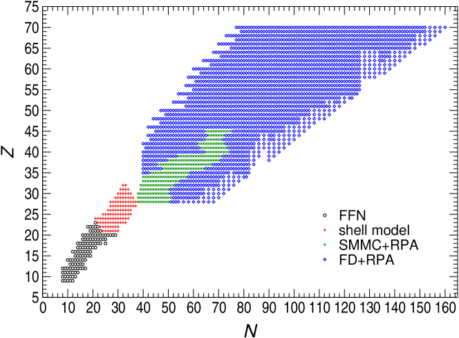
Figure 1: (Color online) Nuclei included in the calculation of the NSE-averaged rates and spectra. The $sd$ pool is marked by circles, the shell model pool is marked by plusses, the SMMC+RPA pool is marked by crosses, and the FD+RPA pool is marked by diamonds.

To have an overview of the pools, Fig. 1 shows the nuclei included in our rate evaluation distinguishing the method used for the individual rates. With four approaches all contributing, validation is an important consideration. Ideally, one would validate the various approaches against experimental data. Unfortunately, such a procedure is severely limited by the lack of data for excited states, while the relative weight of the ground state in the thermal ensemble at temperatures present in the collapsing core is rapidly decreasing. Furthermore, the important role played by the phase space has to be recognized as well. The electron chemical potential grows significantly faster than the average $Q$-values of nuclei present in the core. As a consequence, the stellar electron capture rates are sensitive to detailed Gamow-Teller distributions only at low densities. At higher densities it suffices that the total GT strength and its energy centroid are well described. This calls for more elaborate nuclear models to be used to derive the capture rates for nuclei at low densities than is required for the rates needed at larger densities. We have considered these facts in our strategy for the validation process. At low densities, which is also at low temperatures when nuclei are present, the ground states contribute relatively strongly to the capture rates. For such conditions the core composition is dominated by nuclei with the mass numbers $A=45$–$65$ for which the shell model diagonalization calculation can be performed. Such shell model rates are adopted here. It has been proven by extensive comparison to experiment that the shell model describes measured $GT_{+}$ strength distributions in this mass range very well and also gives a very good account of the spectra at low excitation energies [20, 21, 22, 41]. By the time nuclei with $A>65$, for which shell model diagonalization calculation are prohibitive due to computational restrictions, dominate the core composition, the density, and accordingly the electron chemical potential, has grown sufficiently that the capture rates are mainly sensitive to the total GT strength and its centroid. For such nuclei we have performed RPA calculations with the occupation numbers determined from SMMC calculations or from the simple FD parametrization. This procedure is validated by comparing the shell model and SMMC+RPA results for selected nuclei, indeed finding good agreement, if the electron chemical potential is appropriately large. Finally we derive a simple parametrization of the SMMC occupation numbers and show that this FD parametrization reproduces the SMMC+RPA capture rates quite well. Such a comparison of the rates in the overlapping regions together with the outlined reasoning on the rate sensitivity to the conditions gives us confidence that the approach used is valid.

Having produced the individual rates, we have derived the NSE-averaged electron capture rates for the appropriate conditions during the collapse based on the pool of nearly $2700$ nuclei. An extended tabulation of the capture rates and the corresponding neutrino spectra is available in electronic form upon request from the authors for a wide grid of stellar conditions (defined by temperature, the matter density and the electron-to-baryon ratio). This tabulation is most appropriate for the study of core collapse supernovae, where the large range of density and the neutrino spectral information are necessary. This tabulation is also appropriate for use in thermonuclear supernovae, where the range of density and electron fraction are a subset of those occurring in core collapse supernovae, however the value of the wider nuclear range and neutrino spectral data considered here is lost. Thus for the thermonuclear supernova problem, this tabulation is essentially equivalent to that of Seitenzahl et al. [42], which also folds LMP reactions over an NSE abundance distribution. This tabulation is wholly inappropriate for the study of electron capture in X-ray burst ashes (see, e.g. [43]), because the ash temperature is insufficient to justify the use of NSE.

The paper is organized as follows. Section 2 describes the hybrid model and some computational details. Screening corrections to the rates are also introduced there, but the corresponding formalism is presented in an appendix. Section 3 discusses the obtained results. We conclude with section 4.

2 Theoretical model

The hybrid SMMC+RPA model was proposed in [26] to compute electron capture rates on nuclei which required such large model spaces for which diagonalization shell model calculations are not yet feasible. The hybrid model is computationally feasible, but simultaneously incorporates relevant nuclear structure physics as configuration mixing (caused by nucleon correlations) and thermal effects. A pairing+quadrupole residual interaction [44] was used which avoids the sign problem associated with using realistic interactions in SMMC studies [25]. SMMC calculations at finite temperature are used to obtain occupation numbers for the various neutron and proton valence shells in the parent nucleus, which are then used to calculate electron capture cross sections and rates within a Random Phase Approximation (RPA) approach with partial shell occupancies (the method is explained in Ref. [45]).

We have performed hybrid SMMC+RPA calculations of electron capture rates for additional nuclei extending the pool of nuclei used in [23, 31] to more neutron-rich nuclei and filling occasional holes in isotopic chains. As mentioned above, the first step in the hybrid approach is to obtain the shell occupation numbers for protons and neutrons using the SMMC. Using the same interaction and model space as in [31] (i.e. full $pf$-$gds$ shells with $50$ valence orbitals for protons and neutrons), we have calculated such occupation numbers at finite temperatures for $168$ nuclei with $N\leq 61$. For nuclei with even larger neutron number we switched to the $f_{5/2}p$-$gds$-$h_{11/2}$ model space, changing the pairing and quadrupole strength parameters of the residual interaction to account for the change in the model space. These parameters were adjusted such as both model spaces predict similar properties for selected nuclei. The single-particle energies were taken from [46]. The energy of the $h_{11/2}$ was determined using the same Woods-Saxon parameters as in [46] placing it at $15.12$ MeV above the $f_{7/2}$ shell.

The radial wave functions as well as single-particle energies for the RPA calculation (i.e. the second step for the hybrid method) were taken from the Woods-Saxon potential:

$$V(r) = V_{0}\ \left[1+\exp\left\{\frac{r-R}{a}\right\}\right]^{-1},$$

$$V_{LS} = \frac{1}{2}\lambda\left(\frac{\hbar}{Mc}\right)^{2}\,\frac{1}{r}\frac{\textrm{d}V(r)}{\textrm{d}r}\,{\vec{\ell}\cdot\vec{s}},$$ (1)

$$V_{Coul} = (Z-1)\,\frac{e^{2}}{r}\,\times\ \left\{\begin{array}[]{ll}\frac{3}{2}\frac{r}{R}-\left(\frac{r}{R}\right)^{3}&,\ r<R\\ 1&,\ r\geq R\end{array}\right.$$ (4)

The depth of the potential was adjusted to reproduce the proton separation energy in the parent nucleus and the neutron separation energy in the daughter nucleus, as discussed in [34]. Other parameters of the Woods-Saxon potential were: $r_{0}=1.27$ fm, $R=r_{0}A^{1/3}$, $a=0.65$ fm, $\lambda=32.$ The separation energies were calculated using masses from the Audi et al compilation [40], supplemented by predictions from the finite-range droplet model [39]. The same masses were used to evaluate the $Q$ value for the calculation of electron capture cross sections as will be discussed later.

Following the spirit of RPA+BCS calculations we have shifted the energies of the unoccupied proton states by the amount of the pairing energy estimated as $12/\sqrt{A}$ MeV to avoid the appearance of spurious zero energy transitions in situations where orbits are partially filled. It should be noted that this energy shift does not affect the physical transitions that take place between occupied proton states and unoccupied neutron states. Ref. [31] has used a constant energy shift of 2.5 MeV which leads to slightly larger capture rates. For consistency we have repeated the calculations of the capture rates for the LMS pool of nuclei with the $A$-dependent energy shift.

In the RPA calculations we used the Landau-Migdal force as the residual interaction with the parameters taken from [47], except for the overall scale factor $C_{0}=302$ MeV fm³ [48]. In the calculation of the rates we included all multipole transitions with $J\leq 3$. The dependence of the operators on momentum transfer has been considered which leads to a reduction of the capture cross sections at high electron energies [23]. Motivated by global RPA calculations for muon capture on nuclei [49, 50], the $J=1^{+}$ multipole transitions have been quenched by a factor of $(0.7)^{2}$ but not the other.

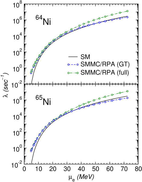
Figure 2: (Color online) A comparison of the electron capture rates on ^64,65Ni calculated from the diagonalization shell model (only allowed contributions) and the hybrid SMMC+RPA model (both allowed and forbidden contributions). Stellar conditions of the $25M_{\odot}$ trajectory (see Table 1) are used.

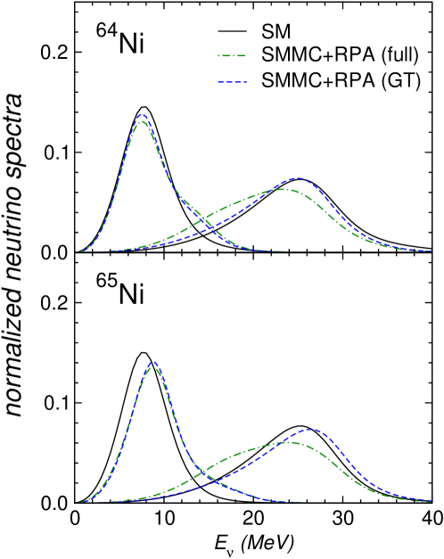
Figure 3: (Color online) A comparison of the neutrino spectra emitted during electron capture on ^64,65Ni calculated from the diagonalization shell model (only allowed contributions) and the hybrid SMMC+RPA model (both allowed and forbidden contributions). Stellar conditions of two zones (10 and 15) of the $25M_{\odot}$ trajectory (see Table 1) are used.

The diagonalization shell model has been clearly established as the method of choice to calculate electron capture rates, provided the required model space is feasible with presently available computer memory. The later restriction, however, prevents its use for many of the heavier neutron-rich nuclei that are present in the collapsing stellar core, forcing us to use the hybrid model as discussed above. We have tested the validity and the accuracy of this hybrid SMMC+RPA approach by comparing electron-capture rates, calculated within this model, against diagonalization shell model results for two nickel isotopes (Fig. 2). The calculations have been performed for a set of stellar conditions (density, temperature, $Y_{e}$ value) appropriate for the inner core of a collapsing $25M_{\odot}$ star (see Table 1). The shell model rates are based only on the allowed Gamow-Teller (GT) transitions, while the SMMC+RPA calculation also includes forbidden transitions. To identify the effect of such forbidden transitions we have also performed SMMC+RPA calculations considering only GT transitions. As can be seen in Fig. 2, the shell model and the hybrid rates are quite similar for electron chemical potentials $\mu_{e}$ larger than about $10$ MeV when only the Gamow-Teller transitions contribute to the electron-capture rate. At lower $\mu_{e}$ values the capture depends more sensitively on the detailed structure of the GT strength distribution which is better described by the diagonalization shell model than in the hybrid model. As explained in [51], with increasing electron chemical potential the capture rate becomes more and more dependent solely on the total GT strength rather than on the details of its distribution. It is fortunate that conditions that produce such low electron chemical potentials, for which a detailed reproduction of the GT strength is required for a reliable description of the rate, also result in relatively low mass nuclei in NSE, for which diagonalization shell model calculations can be performed and which are included in the LMP pool. Forbidden transitions start to contribute noticeably to the capture rates for $\mu_{e}>30$ MeV. At such conditions corresponding to rather high densities the nuclear composition is dominated by nuclei heavier than included in the LMP pool and hence the neglect of higher multipole transitions in the LMP rates is unimportant.

The reasonable reproduction of the shell-model Gamow-Teller distribution by the SMMC+RPA approach is also reflected in the emitted neutrino spectra, shown in Fig. 3. Once the value of the electron chemical potential gets sufficiently large, the emitted neutrino spectra obtained within the shell model and SMMC+RPA approaches are quite similar.

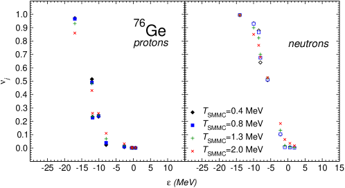
Figure 4: (Color online) Single $j$-shell fractional occupation numbers in ${}_{32}^{76}$Ge at different SMMC temperatures. Proton values are shown on the left, neutron values are shown on the right. The fractional $j$-shell occupancy is calculated by $\nu_{j}=n_{j}/(2j+1)$, where $n_{j}$ is the number of particles in the shell. The single-particle energies are taken from the nucleus-adjusted Woods-Saxon potential.

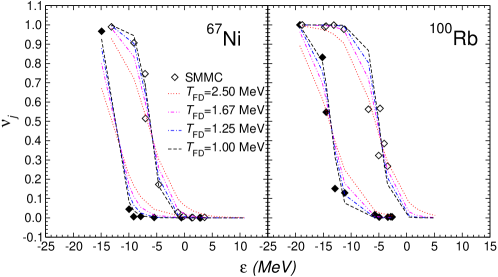
Figure 5: (Color online) Single $j$-shell fractional occupation numbers for ${}_{28}^{67}$Ni and ${}_{\phantom{1}37}^{100}$Rb as a function of single-particle energies. The SMMC results are shown by diamonds; proton values are marked by full symbols, neutron values are marked by empty symbols. The values for ${}_{28}^{67}$Ni and ${}_{\phantom{1}37}^{100}$Rb were obtained at temperatures $T=0.50$ and $1.33$ MeV, respectively. The fractional occupations given by the Fermi-Dirac distribution for four values of $T_{\rm FD}$ are shown by lines: $T_{\rm FD}=2.50$ MeV (dotted), $T_{\rm FD}=1.67$ MeV (dash-double-dotted), $T_{\rm FD}=1.25$ MeV (dash-dotted), $T_{\rm FD}=1.00$ MeV (dashed).

A comment about the occupation numbers used in the SMMC+RPA calculations is in order. In principle one should calculate these numbers at all the temperatures needed to construct the stellar capture rate table. However, such a procedure is computationally untenable. Fortunately it turns out that, within the range of temperatures relevant to the phase of the collapse at which electron captures are important ($T\approx 0.8$–$1.4$ MeV), the occupation numbers do not vary too much. This is demonstrated in Fig. 4 which shows the proton and neutron occupation numbers for ⁷⁶Ge obtained by performing SMMC calculations at different temperatures. We conclude from this comparison that it might suffice to calculate the SMMC occupation numbers only at a single temperature which we chose as the value where the respective nucleus has a large relative weight in the NSE composition.

SMMC calculations are rather time-consuming. Thus calculations to extend the SMMC pool beyond the $250$ nuclei considered here to include the couple of thousand species which are present in the supernova composition is prohibitive. However, the observation that the SMMC occupation numbers do not vary too much with temperature motivated us to find a parameterized form for the SMMC occupation numbers which could then readily be used in RPA calculations of electron capture rates. This goal is achieved by assuming a Fermi-Dirac parameterization for the proton and neutron fractional occupation numbers of various shells with energy $\varepsilon$:

$$\nu_{\rm FD}(\varepsilon,T_{\rm FD})=\frac{1}{1+\exp\{(\varepsilon-\mu)/T_{\rm FD}\}}.$$ (5)

The chemical potentials are fixed by the total proton and neutron numbers (here denoted by $N$)

$$N=\sum\limits_{\varepsilon}\,(2j_{\varepsilon}+1)\,\nu_{\rm FD}(\varepsilon,T_{\rm FD}).$$ (6)

Here $j_{\varepsilon}$ denotes the total angular momentum of a shell having the single-particle energy $\varepsilon$. These energies are taken from a Woods-Saxon potential, the depth of which is adjusted such as the neutron and proton chemical potentials resulting from equation (6) equal the respective neutron and proton separation energies, taken from either experiment or the compilation of ref. [39]. The number of the considered single-$j$ shells depends on the numbers of nucleons and the value of the temperature $T_{\rm FD}$ and exceeds that used in the SMMC studies. The Fermi-Dirac distribution has one more undetermined parameter, $T_{\rm FD}$. We will vary it as a parameter below and fix its value by attempting to reproduce the SMMC+RPA electron capture cross sections for the $250$ nuclei present in the LMS pool. In general we have included at least $2$ major oscillator shells in our RPA calculations outside a closed $N=Z=20$ core.

Fig. 5 compares the SMMC occupation numbers for two different nuclei with those obtained by an FD parameterization for different values of the parameter $T_{\rm FD}$. The values $T_{\rm FD}=1.0$ MeV and $1.25$ MeV give a rather fair reproduction of the SMMC occupation numbers for the two nuclei shown. (As we will see in the next chapter the SMMC+RPA capture cross-sections are globally best reproduced by the value $T_{\rm FD}=1.67$ MeV.) It is important to note that the occupation numbers reflect both correlation and thermal effects. Thus, unlike for a system of non-interacting particles, the parameter $T_{\rm FD}$ should not be interpreted as the temperature of the nucleus.

The stellar electron capture rate $\lambda_{\rm ec}$ on a particular nucleus is related to the electron capture cross-section $\sigma_{\rm ec}$ by:

$$\lambda_{\rm ec}=\frac{1}{\pi^{2}\hbar^{3}}\sum_{if}\int_{\varepsilon_{e}^{0}}^{\infty}p_{e}^{2}\sigma_{\rm ec}(\varepsilon_{e},\varepsilon_{i},\varepsilon_{f})f(\varepsilon_{e},\mu_{e},T)d\varepsilon_{e}$$ (7)

where $\varepsilon_{e}^{0}=\max(Q_{i\!f},m_{e}c^{2})$, $p_{e}=(\varepsilon_{e}^{2}-m_{e}^{2}c^{4})^{1/2}/c$ is the momentum of the incoming electron with energy $\varepsilon_{e}$ and $m_{e}$ the electron rest mass. Under the conditions present in the collapsing core of a supernova, electrons obey a Fermi-Dirac distribution $f(\varepsilon_{e},\mu_{e},T)=[1+\exp\{(\varepsilon_{e}-\mu_{e})/{k_{\rm B}}T\}]^{-1}$ with temperature $T$ and electron chemical potential $\mu_{e}$. $\sigma_{\rm ec}(\varepsilon_{e},\varepsilon_{i},\varepsilon_{f})$ is the cross section for capture of an electron with energy $\varepsilon_{e}$ from an initial proton single particle state with energy $\varepsilon_{i}$ to a neutron single particle state with energy $\varepsilon_{f}$. The cross section is computed within the Random Phase Approximation as described above. Due to energy conservation, the electron, proton and neutron energies are related to the neutrino energy, $\varepsilon_{\nu}$, and the $Q$-value for the capture reaction [34]:

$$Q_{i\!f}=\varepsilon_{e}-\varepsilon_{\nu}=\varepsilon^{n}_{f}-\varepsilon^{p}_{i},$$ (8)

$$\varepsilon^{n}_{f}-\varepsilon^{p}_{i}=\varepsilon^{*}_{if}+\hat{\mu}+\Delta_{np}.$$ (9)

Here we take $\hat{\mu}=\mu_{n}-\mu_{p}$, the difference between neutron and proton chemical potentials in the nucleus and $\Delta_{np}=(M_{n}-M_{p})c^{2}=1.293$ MeV, the neutron-proton mass difference.

Equation (9) constitutes the definition of the quantity $\varepsilon^{*}_{if}$. At zero temperature $\varepsilon^{*}_{if}$ corresponds to the excitation energy in the daughter nucleus. For the transition from the initial ground state to the daughter ground state the excitation energy must be zero. This fact is used for fixing the value of $\hat{\mu}$:

$$Q_{00}=(M_{f}-M_{i})c^{2}=\hat{\mu}+\Delta_{np},$$ (10)

where $M_{i}$ and $M_{f}$ are the nuclear masses of the parent and daughter nuclei in the electron capture reaction, and the values of $\mu_{p}$ and $\mu_{n}$ are selected to equal proton and neutron separation energies, $S_{p}(Z,N)$ and $S_{n}(Z-1,N+1)$. At finite temperature the value of $\varepsilon^{*}_{if}$ can be negative when the nucleus is de-excited by capturing an electron.

The capture rate for individual nuclei is affected by screening corrections that are implemented in our calculations as discussed in the appendix. The screening corrections affect the electron capture in two ways: they effectively increase the $Q$ value and lower the electron chemical potential. As discussed in the next section and the appendix, both effects lead to a reduction of the electron capture rate in the medium as compared to the undisturbed case.

Calculation of the partial cross sections allows us to obtain the spectrum of the emitted neutrinos. To have the spectrum normalized to unity, we define it as follows:

$${\cal N}^{\nu}(\varepsilon_{\nu})=\frac{1}{\lambda_{\rm ec}}\,\frac{1}{\pi^{2}\hbar^{3}}\sum_{if}p_{e}^{2}\sigma_{\rm ec}(\varepsilon_{e},\varepsilon_{i},\varepsilon_{f})f(\varepsilon_{e},\mu_{e},T),$$ (11)

with $\varepsilon_{e}=\varepsilon_{f}-\varepsilon_{i}+\varepsilon_{\nu}$ and $p_{e}$ the corresponding electron momentum. Equation (11) defines the spectrum of emitted neutrinos as produced by captures on a particular nucleus.

During stellar collapse, the matter is composed of individual nuclei until densities of order $10^{13}$ g/cm³ are reached. While presupernova studies (i.e. simulations which cover the late-stage evolution of a massive star until the inner core has reached densities up to $10^{9}$ g/cm³) require explicit consideration of the extensive nuclear networks, temperatures in the subsequent supernova collapse phase are high enough to bring reactions mediated by the strong and electromagnetic force into equilibrium with their inverse reactions and hence the nuclear composition can be described by Nuclear Statistical Equilibrium (NSE). It is customary to split the required electron capture rates for supernova simulations into rates for protons $R_{p}=Y_{p}\lambda_{p}$, and for nuclei $R_{h}=\sum_{i}Y_{i}\lambda_{i}$ where the index $i$ runs over all isotopes other than protons present in the stellar composition. The required abundances for protons $Y_{p}$ and for the various nuclear species $Y_{i}$ are derived from a Saha-like NSE distribution of the individual isotopes where we included consideration of degenerate nucleons and plasma corrections to the nuclear binding energy [52] using the screening formula of Slattery et al [53] with the parameters from [54] and the extension to the weak screening regime as suggested by Yakovlev and Shalybkov [55] as discussed in the appendix. Compared to the LMSH tabulation used in [31, 32], we have extended the pool of nuclei in the NSE distribution to heavier nuclei (Ag to At). Furthermore we have used recently published partition functions which extend to temperatures in excess of $10$ GK [56]. The electron chemical potential necessary for the calculation of the different electron capture rates are determined using the helmholtz Equation of State by Timmes and Swesty [57].

In [31, 32] the stellar electron capture rate $\langle\lambda_{\rm ec}\rangle$ has been derived as the NSE-average over all nuclei for which individual rates are available. Hence,

$$\langle\lambda_{\rm ec}\rangle\,=\,\frac{\sum_{i}\,Y_{i}\lambda_{i}^{\rm ec}}{\sum_{i}\,Y_{i}}$$ (12)

Similarly, the NSE-averaged neutrino spectrum is obtained by calculating the ratio

$$\langle{\cal N}_{\nu}(E_{\nu})\rangle\ =\ \frac{1}{\langle\lambda_{\rm ec}\rangle}\,\frac{\sum_{i}Y_{i}{\cal N}_{i}^{\nu}(\varepsilon_{\nu})\lambda_{i}^{\rm ec}}{\sum_{i}Y_{i}}\ =\ \frac{\sum_{i}Y_{i}{\cal N}_{i}^{\nu}(\varepsilon_{\nu})\lambda_{i}^{\rm ec}}{\sum_{i}Y_{i}\lambda_{i}^{\rm ec}}$$ (13)

This spectrum is normalized to unity, with the absolute neutrino emission rate being $\langle\lambda_{\rm ec}\rangle\langle{\cal N}_{\nu}(E_{\nu})\rangle$.

Table 1: Conditions for a central mass element in two progenitor stars at several points in time during the collapse. $\bar{A}$ and $\bar{Z}$ is the average mass and proton numbers as given by the NSE. $Y_{p}$ is the abundance of protons. $Y_{h}$ is the abundance of heavy nuclei defined as $Y_{h}=(\sum Y_{i})-Y_{p}-Y_{n}-Y_{\alpha}$, i.e. everything except for protons, neutrons and alpha particles. $Z_{h}$ and $A_{h}$ are the average mass and charge of the heavy nuclei. The last two columns list values of the unscreened and screened electron capture rates ($\langle\lambda_{\rm ec}^{\rm ns}\rangle$ and $\langle\lambda_{\rm ec}\rangle$, respectively).

idx	$\rho$	$Y_{e}$	$T$	$k_{B}T$	$\mu_{e}$	${\bar{A}}$	${\bar{Z}}$	${\bar{A}}_{h}$	${\bar{Z}}_{h}$	$Y_{p}$	$Y_{h}$	$Y_{p}/Y_{h}$	$\langle\lambda_{\rm ec}^{\rm ns}\rangle$	$\langle\lambda_{\rm ec}\rangle$
	(g/cm3)		(GK)	(MeV)	(MeV)					(mol/g)	(mol/g)		(sec-1)	(sec-1)
$15M_{\odot}$ progenitor										$\times 10^{-5}$	$\times 10^{-2}$	$\times 10^{-3}$
1	$8.56\times 10^{9}$	0.434	$7.49$	$0.65$	$7.83$	$58.0$	$25.2$	$60.2$	$26.1$	$0.230$	$1.66$	$0.139$	$1.94\times 10^{0}$	$1.38\times 10^{0}$
2	$9.34\times 10^{9}$	0.434	$7.73$	$0.67$	$8.06$	$57.4$	$24.9$	$60.3$	$26.2$	$0.349$	$1.65$	$0.211$	$2.62\times 10^{0}$	$1.87\times 10^{0}$
3	$1.34\times 10^{10}$	0.431	$8.78$	$0.76$	$9.04$	$52.1$	$22.5$	$61.2$	$26.4$	$1.61$	$1.62$	$0.991$	$8.15\times 10^{0}$	$5.83\times 10^{0}$
4	$2.42\times 10^{10}$	0.422	$10.02$	$0.88$	$10.97$	$40.8$	$17.2$	$64.6$	$27.4$	$5.24$	$1.52$	$3.44$	$4.10\times 10^{1}$	$2.96\times 10^{1}$
5	$4.71\times 10^{10}$	0.403	$11.39$	$0.98$	$13.53$	$30.1$	$12.1$	$73.2$	$30.0$	$4.22$	$1.33$	$3.17$	$1.47\times 10^{2}$	$1.05\times 10^{2}$
6	$6.95\times 10^{10}$	0.391	$11.91$	$1.03$	$15.27$	$24.1$	$9.4$	$77.1$	$30.9$	$2.50$	$1.26$	$2.00$	$2.14\times 10^{2}$	$1.50\times 10^{2}$
7	$1.12\times 10^{11}$	0.377	$12.64$	$1.09$	$17.76$	$17.9$	$6.7$	$79.1$	$31.1$	$1.53$	$1.21$	$1.27$	$3.31\times 10^{2}$	$2.24\times 10^{2}$
8	$1.83\times 10^{11}$	0.365	$13.57$	$1.17$	$20.69$	$14.0$	$5.1$	$79.9$	$31.0$	$1.33$	$1.17$	$1.13$	$6.96\times 10^{2}$	$4.50\times 10^{2}$
9	$2.33\times 10^{11}$	0.359	$14.11$	$1.22$	$22.35$	$12.4$	$4.5$	$80.3$	$31.0$	$1.32$	$1.16$	$1.14$	$1.10\times 10^{3}$	$6.97\times 10^{2}$
10	$3.76\times 10^{11}$	0.344	$15.26$	$1.32$	$25.84$	$9.6$	$3.3$	$81.7$	$30.9$	$1.17$	$1.11$	$1.05$	$2.68\times 10^{3}$	$1.64\times 10^{3}$
11	$5.89\times 10^{11}$	0.319	$16.22$	$1.40$	$29.33$	$7.1$	$2.3$	$85.7$	$31.5$	$0.646$	$1.01$	$0.637$	$5.70\times 10^{3}$	$3.36\times 10^{3}$
12	$9.33\times 10^{11}$	0.295	$17.51$	$1.51$	$33.31$	$5.5$	$1.6$	$93.0$	$33.2$	$0.471$	$0.888$	$0.530$	$1.37\times 10^{4}$	$7.76\times 10^{3}$
13	$1.53\times 10^{12}$	0.284	$19.82$	$1.71$	$38.79$	$5.0$	$1.4$	$98.1$	$34.5$	$0.884$	$0.823$	$1.07$	$4.67\times 10^{4}$	$2.60\times 10^{4}$
14	$1.95\times 10^{12}$	0.280	$20.99$	$1.81$	$41.82$	$4.8$	$1.4$	$100.2$	$34.9$	$1.09$	$0.799$	$1.36$	$8.30\times 10^{4}$	$4.60\times 10^{4}$
15	$2.47\times 10^{12}$	0.275	$22.37$	$1.93$	$45.04$	$4.7$	$1.3$	$101.5$	$35.1$	$1.40$	$0.782$	$1.79$	$1.46\times 10^{5}$	$8.06\times 10^{4}$
16	$3.17\times 10^{12}$	0.272	$24.08$	$2.08$	$48.76$	$4.6$	$1.3$	$101.8$	$34.9$	$2.04$	$0.777$	$2.63$	$2.72\times 10^{5}$	$1.51\times 10^{5}$
17	$4.04\times 10^{12}$	0.269	$25.54$	$2.20$	$52.72$	$4.6$	$1.2$	$103.9$	$35.3$	$2.32$	$0.762$	$3.05$	$4.91\times 10^{5}$	$2.70\times 10^{5}$
18	$5.14\times 10^{12}$	0.263	$27.06$	$2.33$	$56.70$	$4.5$	$1.2$	$106.8$	$35.8$	$2.39$	$0.736$	$3.25$	$8.23\times 10^{5}$	$4.47\times 10^{5}$
19	$6.59\times 10^{12}$	0.259	$29.43$	$2.54$	$61.27$	$4.5$	$1.2$	$106.5$	$35.2$	$3.32$	$0.735$	$4.52$	$1.47\times 10^{6}$	$7.92\times 10^{5}$
20	$8.51\times 10^{12}$	0.261	$32.12$	$2.77$	$66.88$	$4.7$	$1.2$	$105.6$	$34.7$	$4.98$	$0.750$	$6.63$	$2.99\times 10^{6}$	$1.58\times 10^{6}$
21	$1.07\times 10^{13}$	0.260	$33.76$	$2.91$	$72.14$	$4.8$	$1.2$	$111.3$	$36.1$	$4.61$	$0.719$	$6.41$	$5.18\times 10^{6}$	$2.67\times 10^{6}$

Continuation of Table 1

idx	$\rho$	$Y_{e}$	$T$	$k_{B}T$	$\mu_{e}$	${\bar{A}}$	${\bar{Z}}$	${\bar{A}}_{h}$	${\bar{Z}}_{h}$	$Y_{p}$	$Y_{h}$	$Y_{p}/Y_{h}$	$\langle\lambda_{\rm ec}^{\rm ns}\rangle$	$\langle\lambda_{\rm ec}\rangle$
	(g/cm3)		(GK)	(MeV)	(MeV)					(mol/g)	(mol/g)		(sec-1)	(sec-1)
$25M_{\odot}$ progenitor										$\times 10^{-4}$	$\times 10^{-2}$	$\times 10^{-2}$
1	$2.22\times 10^{9}$	0.447	$7.86$	$0.68$	$4.87$	$44.8$	$20.0$	$56.4$	$25.1$	$0.788$	$1.74$	$0.451$	$8.99\times 10^{-2}$	$6.65\times 10^{-2}$
2	$2.97\times 10^{9}$	0.445	$8.44$	$0.73$	$5.38$	$39.3$	$17.5$	$56.5$	$25.1$	$1.46$	$1.72$	$0.845$	$2.04\times 10^{-1}$	$1.51\times 10^{-1}$
3	$5.59\times 10^{9}$	0.435	$9.83$	$0.85$	$6.61$	$25.4$	$11.0$	$57.4$	$25.1$	$3.09$	$1.64$	$1.88$	$9.77\times 10^{-1}$	$7.32\times 10^{-1}$
4	$6.74\times 10^{9}$	0.431	$10.22$	$0.88$	$7.03$	$22.3$	$9.6$	$57.9$	$25.1$	$3.56$	$1.61$	$2.21$	$1.58\times 10^{0}$	$1.19\times 10^{0}$
5	$9.79\times 10^{9}$	0.425	$10.81$	$0.93$	$7.96$	$19.4$	$8.2$	$58.9$	$25.4$	$3.92$	$1.57$	$2.50$	$4.04\times 10^{0}$	$3.02\times 10^{0}$
6	$1.46\times 10^{10}$	0.418	$11.44$	$0.99$	$9.09$	$17.1$	$7.1$	$60.5$	$25.8$	$4.09$	$1.52$	$2.69$	$1.08\times 10^{1}$	$7.99\times 10^{0}$
7	$2.49\times 10^{10}$	0.407	$12.10$	$1.04$	$10.84$	$16.0$	$6.5$	$64.2$	$26.9$	$3.15$	$1.44$	$2.19$	$3.73\times 10^{1}$	$2.74\times 10^{1}$
8	$4.26\times 10^{10}$	0.395	$12.72$	$1.10$	$12.92$	$15.3$	$6.0$	$69.1$	$28.4$	$2.04$	$1.35$	$1.51$	$1.09\times 10^{2}$	$7.92\times 10^{1}$
9	$6.91\times 10^{10}$	0.384	$13.35$	$1.15$	$15.10$	$14.0$	$5.4$	$73.3$	$29.6$	$1.36$	$1.27$	$1.07$	$2.41\times 10^{2}$	$1.71\times 10^{2}$
10	$1.13\times 10^{11}$	0.372	$14.11$	$1.22$	$17.68$	$12.2$	$4.5$	$76.3$	$30.4$	$0.934$	$1.21$	$0.772$	$4.85\times 10^{2}$	$3.35\times 10^{2}$
11	$1.88\times 10^{11}$	0.361	$15.11$	$1.30$	$20.75$	$10.3$	$3.7$	$77.9$	$30.6$	$0.752$	$1.17$	$0.644$	$1.07\times 10^{3}$	$7.10\times 10^{2}$
12	$3.75\times 10^{11}$	0.339	$16.76$	$1.44$	$25.66$	$7.8$	$2.6$	$79.9$	$30.6$	$0.532$	$1.10$	$0.483$	$3.42\times 10^{3}$	$2.13\times 10^{3}$
13	$5.92\times 10^{11}$	0.315	$17.79$	$1.53$	$29.17$	$6.0$	$1.9$	$83.1$	$30.9$	$0.291$	$1.01$	$0.287$	$6.81\times 10^{3}$	$4.08\times 10^{3}$
14	$9.41\times 10^{11}$	0.291	$19.32$	$1.67$	$33.23$	$4.9$	$1.4$	$87.8$	$31.8$	$0.234$	$0.915$	$0.256$	$1.64\times 10^{4}$	$9.54\times 10^{3}$
15	$1.54\times 10^{12}$	0.281	$21.84$	$1.88$	$38.68$	$4.5$	$1.3$	$90.1$	$32.1$	$0.376$	$0.871$	$0.432$	$5.41\times 10^{4}$	$3.10\times 10^{4}$
16	$1.97\times 10^{12}$	0.275	$23.21$	$2.00$	$41.74$	$4.3$	$1.2$	$90.7$	$32.0$	$0.446$	$0.858$	$0.520$	$9.53\times 10^{4}$	$5.43\times 10^{4}$
17	$2.53\times 10^{12}$	0.271	$24.90$	$2.15$	$45.09$	$4.2$	$1.1$	$89.6$	$31.4$	$0.587$	$0.861$	$0.682$	$1.70\times 10^{5}$	$9.70\times 10^{4}$
18	$3.25\times 10^{12}$	0.269	$26.78$	$2.31$	$48.90$	$4.2$	$1.1$	$87.9$	$30.5$	$0.777$	$0.876$	$0.887$	$3.18\times 10^{5}$	$1.81\times 10^{5}$
19	$4.14\times 10^{12}$	0.265	$28.43$	$2.45$	$52.77$	$4.2$	$1.1$	$88.0$	$30.2$	$0.832$	$0.874$	$0.952$	$5.47\times 10^{5}$	$3.09\times 10^{5}$
20	$5.28\times 10^{12}$	0.259	$30.43$	$2.62$	$56.84$	$4.1$	$1.1$	$87.0$	$29.5$	$0.916$	$0.877$	$1.04$	$9.20\times 10^{5}$	$5.14\times 10^{5}$
21	$6.79\times 10^{12}$	0.257	$33.24$	$2.86$	$61.65$	$4.1$	$1.1$	$82.9$	$27.8$	$1.26$	$0.922$	$1.37$	$1.71\times 10^{6}$	$9.47\times 10^{5}$
22	$8.75\times 10^{12}$	0.258	$35.99$	$3.10$	$67.18$	$4.3$	$1.1$	$81.3$	$27.0$	$1.58$	$0.952$	$1.65$	$3.33\times 10^{6}$	$1.82\times 10^{6}$
23	$1.11\times 10^{13}$	0.256	$37.99$	$3.27$	$72.40$	$4.4$	$1.1$	$84.8$	$27.7$	$1.42$	$0.919$	$1.55$	$5.59\times 10^{6}$	$2.98\times 10^{6}$

However, there is a potential problem with the average rate as defined above, when applied to the pool of nuclei used in [31, 32], as this pool was limited to nuclei with mass numbers $A<112$, sampling only a rather small fraction of the total NSE abundance in the later phase of the collapse (changes in nuclear composition during the collapse are illustrated in [58]). While this averaging of the rate prevents the total rate of electron capture from unphysically dropping to zero as the fraction of nuclei with calculated rates declines, the average rate becomes increasingly dominated by the species at the neutron-rich edge of the calculated pools, making the averaged rates of [31, 32] uncertain. It is the aim of the present work to overcome this shortcoming by appropriately enlarging the pool of nuclei from which the averages (12) and (13) are being derived. The present pool contains nearly $2700$ nuclei (in contrast to about $280$ considered in [31, 32]). For nuclei with mass numbers $A<65$ our pool consists of the LMP shell model rates [22] (i.e. the $pf$-shell nuclei) supplemented by the FFN rates for the lighter $sd$-shell nuclei. We have also extended the pool of nuclei for which rates are based on the hybrid SMMC+RPA approach to include nuclei up to $A=120$ (SMMC pool). The pool is completed by more than $2500$ nuclei for which we have derived rates based on RPA calculations with the occupation numbers approximated by the parameterized FD distribution as discussed above (FD pool). As some of the nuclei calculated within this approach are overlapping with the nuclei from other pools, we do not use the FD+RPA results if the rates and spectra are already provided by other pools, unless specifically indicated.

In the next section we present electron capture rates and the emitted neutrino spectra for conditions during the core collapse of two progenitor stars with different masses. The first set of conditions follows a central mass element (at an enclosed mass of $0.05$ solar masses) during the collapse of a $15M_{\odot}$ progenitor star derived from a simulation using electron-capture rates from the LMSH tabulation [31, 32] and general relativity. The second set is based on a similar simulation, but for a $25M_{\odot}$ progenitor star. The stellar conditions are defined in Table 1.

3 Results and discussion

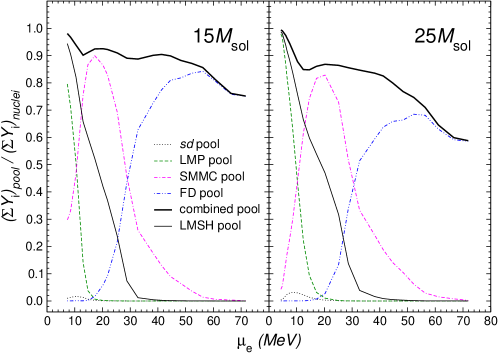
Figure 6: (Color online) Fraction of nuclei covered by the various pools of nuclei as defined in the text. The fractions have been calculated for the two stellar trajectories given in Table 1. The pools are $sd$ (dotted line), LMP (dashed line), SMMC+RPA (double-dash-dotted line), and FD+RPA (dash-double-dotted line). Solid lines show the summed pool coverage. Thick solid lines show present pool coverage, and thin solid lines show coverage by the LMSH pool. $(\sum_{i}Y_{i})_{\rm nuclei}$ is calculated by summing over all nuclei except protons, neutrons and $\alpha$ particles.

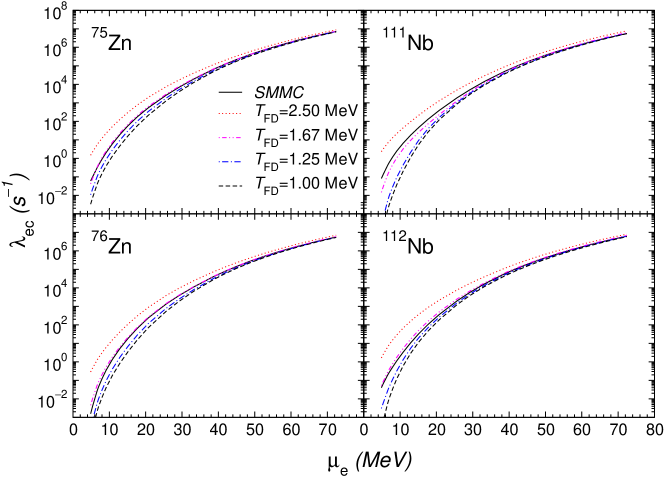
Figure 7: (Color online) Electron capture rates for four nuclei from the SMMC pool: ^75,76Zn, ^111,112Nb. The SMMC+RPA rates are shown by solid lines. The FD+RPA rates have been calculated for $T_{\rm FD}=2.50$ MeV (dotted line), $T_{\rm FD}=1.67$ MeV (dash-double-dotted line), $T_{\rm FD}=1.25$ MeV (dash-dotted line), and $T_{\rm FD}=1.00$ MeV (dashed line). The stellar conditions are those of $25M_{\odot}$ progenitor star (Table 1).

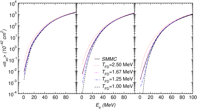
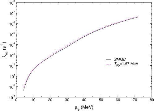
Figure 8: (Color online) NSE-averaged electron-capture cross-sections as calculated by the SMMC+RPA and FD+RPA approaches for the $250$ nuclei of the SMMC+RPA pool at three stellar conditions of the $25M_{\odot}$ trajectory: the snapshot number 4 is used in the left panel, the number 10 in the center panel, and the number 13 in the right panel. The notation is the same as in Fig. 7.

Figure 9: (Color online) NSE-averaged electron-capture rates as calculated by the SMMC+RPA and FD+RPA approaches for the $250$ nuclei of the SMMC+RPA pool. The stellar conditions are those of $25M_{\odot}$ progenitor star (Table 1). The solid line shows the SMMC+RPA rate. The dashed line gives the FD+RPA rates calculated with $T_{\rm FD}=1.67$ MeV.

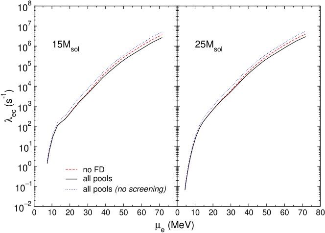
Figure 10: (Color online) Pool-averaged electron-capture rates calculated along the stellar trajectories for the $15M_{\odot}$ and $25M_{\odot}$ progenitor stars. The rates based on the sum of all pools of nuclei are shown by solid lines. The dashed lines show the average rate when the FD+RPA pool is omitted. The dotted lines show the average rate for the sum of all pools when the screening effects to the rates are neglected.

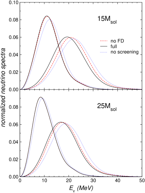
Figure 11: (Color online) Pool-averaged emitted neutrino spectra for the $15M_{\odot}$ and $25M_{\odot}$ trajectories. The line legend is the same as in Fig. 10. Two stellar conditions are used in each case corresponding to snapshot numbers 10 and 15 of the respective trajectory. For snapshot number 10 in the lower panel the curves “no FD” and “full” coincide.

As mentioned above, the pool of nuclei adopted to derive the LMSH electron capture tabulation used in [31, 32] was limited to isotopes with $A<112$ and turns out to cover only a small fraction of the total NSE abundance in the latest stages of the collapse for two reasons. First, heavier nuclei appear in the nuclear composition with noticeable abundances. Secondly, the inclusion of electron capture on nuclei makes the matter more neutron-rich than anticipated in prior studies which considered only capture on protons and neglected the dominant electron reducing weak process. As the pool of nuclei used in [31] has been constructed based on trajectories from prior collapse simulations which solely considered capture on protons, the pool was missing relevant neutron-rich isotopes.

The limitation of the nuclear pool used in [31] (LMSH pool, i.e. the combined $sd$, LMP and LMS pools) is shown in Fig. 6. This sample is complete for the early stage of the collapse ($\mathrel{\lesssim}10^{10}$ g/cm³) where the pool includes more than $90\%$ of the nuclei present in the supernova medium (indices 1-3 of the $15M_{\odot}$ and 1-4 of the $25M_{\odot}$ trajectories in Table 1). However, the coverage drops quickly as the collapse progresses. The pool covers more than $50\%$ of the total NSE abundance for densities $\mathrel{\lesssim}10^{11}$ g/cm³(indices 7 and 10 respectively). At the conditions around neutrino trapping (indices 10 and 12, respectively, of the $15M_{\odot}$ and $25M_{\odot}$ collapse trajectories) only $20\%$ of the total NSE abundance is sampled by the LMSH pool. This drastic underrepresentation is improved slightly by including the additional $170$ nuclei for which we have calculated capture rates using the SMMC+RPA approach, pushing the limits at which the $20\%$ coverage of the total NSE abundance is reached to indices 11 and 15 for the $15M_{\odot}$ and $25M_{\odot}$ trajectories, respectively.

Obviously improving the coverage requires an appropriate enlargement of the nuclear pool from which the capture rates are derived. This is in particular motivated by the fact that the omission of the neutron-rich nuclei from the pool in [31] could result in a systematic overestimate of the rates as the capture process gets increasingly hindered with growing neutron excess due to Pauli blocking. However, covering the relevant nuclei by SMMC+RPA calculations is too computationally demanding. Thus we have performed evaluations of the capture rates for more than $2200$ nuclei using occupation numbers derived from a FD parameterization. These nuclei consider the isotope chains for charge numbers $Z=28$–$70$. When these nuclei are added to the pool, Fig. 6 shows that at least $60\%$ of the total NSE abundance is considered during the entire collapse evolution until densities of order $10^{13}$ g/cm³ are reached and the description of the nuclear composition by individual nuclei is inadequate. We stress that at the beginning of the core collapse, the center of a progenitor star is populated by iron group nuclei, therefore electrons are mostly captured by the nuclei from the LMP pool. As the collapse progresses, the nuclei become heavier and more neutron rich. Nuclei from the SMMC+RPA pool dominate the rates at densities from $5\times 10^{10}$ g/cm³ to neutrino trapping around $5\times 10^{11}$ g/cm³. At even higher densities nuclei from the FD+RPA pool dominate the rates.

The FD+RPA approach is considered as an approximation to SMMC+RPA calculations. To verify its validity we previously compared the FD-predicted occupation numbers to those obtained from the SMMC calculation and found fair agreement (Fig. 5). The SMMC occupation numbers show some deviation from the smooth FD behavior, caused by correlations introduced by the residual interaction, and not reproduced by the FD distribution. These deviations translate into differences of the rates for individual nuclei (see Fig. 7). However, they do not represent a systematic effect and are smeared out when the averaging over many nuclei takes place. This is demonstrated in Fig. 9 where we compare electron capture cross sections as derived in the SMMC+RPA approach with those obtained in the FD+RPA approximation. The comparison is made for the $250$ nuclei, for which SMMC+RPA rates are now available, adopting for the NSE averaging the stellar conditions of the $25M_{\odot}$ progenitor star (Table 1). We note that the SMMC pool only includes heavy nuclei with charge numbers $Z\geq 28$, while the capture on the lighter $pf$ shell nuclei has been evaluated on the basis of the diagonalization shell model and is here summarized within the LMP pool. Fig. 9 demonstrates the results for the cross section comparison at three distinct points along the stellar trajectory. The left plot corresponds to a rather early stage of the collapse (presupernova phase, index 4) where the SMMC pool covers $81\%$ of the total abundance of heavy nuclei with $Z\geq 28$. The center plot corresponds to collapse conditions just before neutrino trapping sets in (index 10). Here the $250$ nuclei of the SMMC pool contribute $99\%$ of the abundance of heavy nuclei with $Z\geq 28$ and dominate the capture rate in the combined pool. The right plot represents conditions after neutrino trapping (index 13). The coverage of the heavy nuclei abundance by the SMMC pool has now decreased to $60\%$ and the NSE-averaged cross-sections are dominated by the most neutron-rich nuclei included in the pool. The FD+RPA cross sections have been calculated for four different values of the parameter $T_{\rm FD}$. The cross sections at fixed electron energy grow with increasing $T_{\rm FD}$ as more nucleons are excited across the $N=40$ shell gap opening neutron holes in the $pf$ shell and allowing for proton excitations within the $gds$ shell. Differences between the calculations with different values of $T_{\rm FD}$ are most noticeable at low electron energies where the capture process is sensitive to the details of the GT strength distribution. In turn, the agreement between the calculations improves for growing electron energy. We find that the SMMC+RPA results are best reproduced by the NSE-averaged FD+RPA cross sections for $T_{\rm FD}=1.67$ MeV. We will use in the following this value for $T_{\rm FD}$. Fig. 9 shows that the FD+RPA approach with $T_{\rm FD}=1.67$ MeV indeed describes the NSE-averaged SMMC electron capture rates quite well for chemical potentials $\mu_{e}>10$ MeV. This is the regime of interest as we will use the FD+RPA approach to estimate the capture rates for neutron-rich nuclei which only contribute significantly to the total NSE abundance at high densities, i.e. at the conditions for which the electron chemical potential is larger than $30$ MeV.

The discussion above took advantage of the extended SMMC+RPA pool of $250$ nuclei, which is noticeably larger than the one adopted in [31, 32]. This increase in coverage lowered the NSE-averaged rates [38] at higher values of electron chemical potential as many of the added nuclei are more neutron-rich than those used in the original LMSH rates [31]. As explained above, an increase in the neutron excess usually leads to larger Pauli blocking of GT transitions and hence smaller rates. Furthermore, more neutron-rich nuclei have larger $Q$ values which also reduces the electron capture rate.

Finally we compare electron capture rates for different pools of nuclei in Fig. 10. The $sd$+LMP+SMMC+FD pool (“all pools” in the figure legend) considers around $2700$ nuclei, including more than $2200$ nuclei for which the rates have been derived using the FD+RPA approach. The $sd$+LMP+SMMC pool (“no FD” in the legend) leaves out the FD+RPA rates. A comparison between the NSE averaged rates for these pools allows an estimate of the relevance of the omission of the heavy and most neutron-rich nuclei for stellar electron capture. The rates have been calculated for the conditions along the collapse trajectories of the $15M_{\odot}$ and $25M_{\odot}$ progenitor stars as listed in Table 1. (The obtained rates are also given in this table.) As can be observed in Fig. 10 the additional inclusion of the $2200$ heavy and neutron-rich nuclei lowers the NSE-averaged rates at larger electron chemical potential slightly, where the added nuclei dominate.

Fig. 10 also quantitatively demonstrates the impact of the medium effects on the NSE-averaged rate. As mentioned above, screening effects on the electron capture rates lead to a reduction of the electron capture rates which can amount to almost a factor of $2$ at large densities (large chemical potentials in Fig. 10). This is in addition to the effects of screening on the strong and electromagnetic rates that determine the NSE [52, 59], which is included in [31, 32]. Despite this modest reduction in the rates electron capture on nuclei still dominates over capture on free protons during the stellar collapse.

As mentioned in the first section, a very important quantity for supernova simulations is the spectral distribution of the emitted neutrinos which becomes relevant especially at higher densities when neutrinos are becoming trapped. Fig. 11 illustrates the calculated spectra of the neutrinos emitted at different stages of the collapse using the conditions defined by indices 10 and 15 of the collapse trajectories of the $15M_{\odot}$ and $25M_{\odot}$ progenitor stars (Table 1). The neutrino spectra are only slightly changed if we increase the pool of nuclei by more than $2200$ heavy and neutron-rich nuclei. At the beginning of the collapse these nuclei do not contribute (this is especially true for the snapshot number 10 of the $25M_{\odot}$ star, where the lines “full” and “no FD” are indistinguishable in Fig. 11). At $\mu_{e}\approx 20$ MeV, the SMMC+RPA nuclei dominate. For the later collapse phase the inclusion of the FD+RPA nuclei slightly reduces the average neutrino energy, in agreement with the fact that the heavy neutron-rich nuclei have slightly larger $Q$ values.

Already during the construction of the LMSH tabulation [31] it was realized that the shell model approaches can provide rates only for a sample of the nuclei present in the medium of a collapsing star. For nuclei not included in the sample, it was suggested to use a formula based on phase space considerations with parameters fixed to approximately reproduce the rates of nuclei in the pool (eq. (1) in [31]). A more careful study of this proposal revealed a deficiency in this approach [38]. For electron chemical potential above $\mu_{e}>40$ MeV, forbidden transitions contribute significantly, and the value of the “typical” transition matrix element $B$, derived for pure allowed GT transitions, becomes too small. We do not suggest an alternative parameterization of the rates here. However, we would like to exploit the observation that electron capture rates are becoming insensitive to the detailed structure of the nuclear transitions with increasing chemical potential and are then relatively simple functions of $Q$ for a fixed $\mu_{e}$. Using the $250$ nuclei of the SMMC pool we have derived an (unweighted) average rate for fixed values of $(Q,\mu_{e})$. Identifying each of the more than $2200$ nuclei, for which the rate has been calculated solely on the basis of the FD parametrization, by its $Q$ value, we have derived an alternative set of capture rates where the rate of each nucleus, as determined by the FD+RPA approach, has been replaced by the average rate from the SMMC pool at the corresponding values of $Q$ and $\mu_{e}$. The two sets of rates are compared in Fig. 12. The agreement between the sets is excellent, providing confidence that the limitations of FD+RPA approach are of little impact here.

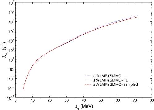
Figure 12: (Color online) Pool-averaged electron capture rates for the trajectory of the $25M_{\odot}$ progenitor star. The rates based on the combined $sd$, LMP and the SMMC+RPA pool is shown by the dotted line. The averaged rate obtained when the FD+RPA pool of rates is also included is shown by the solid line. The dashed line shows the rates if the SMMC-sampled $(Q,\lambda)$ rates (see text) are used to replace the FD+RPA results.

4 Conclusions

Core-collapse supernova simulations require reliable electron-capture (and neutrino emission) rates to track the deleptonization process. In this pursuit we present here an enlarged pool of nuclei from which we derive NSE-averaged electron capture rates and the corresponding emitted neutrino spectra. This extended pool now consists of around $2700$ nuclei. The rates of the $sd$ shell nuclei are taken from Refs. [16, 17, 18, 19], modified by appropriate screening corrections. The $pf$ shell nuclei are adopted from the LMP rates [22]. The SMMC+RPA set [23, 31] was enlarged to include in total $250$ nuclei [38]. Additionally, more than $2200$ nuclei are calculated within the FD+RPA approach, adjusted to reproduce the SMMC+RPA rates. In the FD+RPA approach the parent nucleus occupation numbers at finite temperature are approximated by a Fermi-Dirac parameterization taking the parameter value $T_{\rm FD}=1.67$ MeV. The latter three sets of rates include screening effects directly, while for the FFN rates we use an approximate, but rather accurate, prescription. This huge number of individual electron-capture rates was used to obtain the averaged electron-capture rates at various stellar conditions $(\rho,T,Y_{e})$. The resulting table is available upon request from the authors.

*

Appendix A Screening corrections to electron capture rates

Coulomb corrections are known to play an important role in determining the thermodynamical properties of a high density plasma [55]. At the conditions we are interested in this work the matter can be assumed to be in nuclear statistical equilibrium. This regime has been studied by Bravo and García-Senz [59] and we have generalized their treatment to the study of electron capture rates. When Coulomb corrections are included the chemical potential of the nuclear species is given by:

$$\mu_{i}=\mu_{i,0}+\mu_{i,C}.$$ (14)

Here $\mu_{i,0}$ is the chemical potential in the absence of Coulomb effects which is generally given by the Boltzmann statistics, and $\mu_{i,C}$ is the contribution to the chemical potential due to the interaction of nucleus $i$ with the electron background.

The core of the star constitutes a multicomponent plasma that we will treat in the additive approximation. In this case, all the thermodynamic quantities are computed as the sum of the individual quantities for each species. If one further assumes that the electron distribution is not affected by the presence of the nuclear charges (uniform background approximation), the Coulomb chemical potential of species $i$ is given by [55]

$$\mu_{i,C}=k_{B}Tf_{C}(\Gamma_{i}),$$ (15)

where $f_{C}$ is the Coulomb free energy per ion in units of $k_{B}T$ and $\Gamma_{i}$ is the ion-coupling parameter,

$$\Gamma_{i}=Z_{i}^{5/3}\Gamma_{e}=\frac{Z_{i}^{5/3}e^{2}}{a_{e}k_{B}T},$$ (16)

where $a_{e}$ is the electron sphere radius, $a_{e}=(3/(4\pi n_{e}))^{1/3}$, with $n_{e}$ the electron density.

For the free energy in the regime $\Gamma>1$, we use the expression [55, 60]:

$$f_{C}(\Gamma)=a\Gamma+4b\Gamma^{1/4}-4c\Gamma^{-1/4}+d\ln\Gamma+e,$$ (17)

with the values of the parameters $a,b,c,d$ and $e$ taken from [61]:

$$a = -0.898004,\quad b=0.96786,\quad c=0.220703$$

$$d = -0.86097,\quad e=-2.52692.$$ (18)

For $\Gamma<1$, we use the expression suggested in ref. [55]:

$$f_{C}(\Gamma)=-\frac{1}{\sqrt{3}}\Gamma^{3/2}+\frac{\beta}{\gamma}\Gamma^{\gamma}.$$ (19)

The first term reproduces the Debye-Hückel limit for $\Gamma\ll 1$ and the parameters $\beta$ and $\gamma$ are determined requiring the continuity of the internal energy and its derivative at $\Gamma=1$. These conditions give $\beta=0.295614$ and $\gamma=1.98848$.

The Coulomb corrections contribute to the electron capture rates in two different ways. First, due to the fact that the chemical potential depends on $Z$, screening effects will change the threshold energy for the capture by the amount [62]:

$$\Delta Q_{C}=\mu_{C}(Z-1)-\mu_{C}(Z),$$ (20)

where $Z$ is the charge number of the capturing nucleus. As $\mu_{C}$ is negative, this correction increases the energy threshold and thus reduces the electron capture rate.

Second, the energy of the captured electron is affected by the presence of the background electron gas. Its energy will be reduced compared to the unscreened case. The magnitude of this effect can be determined using linear response theory [63]. Moreover, we can assume that the screening potential, $V_{s}$, is constant inside the nucleus with a value which can be determined from equation (17) of Itoh et al. [63] evaluated at the nuclear radius.

To consider both screening corrections the phase space integral [21] gets modified. The rate of the electron capture during the nuclear transition from an initial state $i$ to a final state $f$  is given by:

$$\lambda^{\rm ec}_{i\!f}=\frac{1}{\pi^{2}\hbar^{3}}\int_{\varepsilon_{e}^{0s}}^{\infty}p_{e}^{2}\sigma_{\rm ec}(\varepsilon_{e},\varepsilon_{i},\varepsilon_{f})f(\varepsilon_{e}+V_{s},\mu_{e},T)d\varepsilon_{e},$$ (21)

$\varepsilon_{e}^{0s}=\max(Q_{i\!f}^{s},m_{e}c^{2})$, and the energy of the emitted neutrino is related to the electron energy by $\varepsilon_{\nu}=\varepsilon_{e}-Q_{i\!f}^{s}$, where

$$Q_{i\!f}^{s}=Q_{i\!f}+\Delta Q_{C},$$ (22)

with $Q_{i\!f}$ being the capture threshold in the absence of screening corrections.

Assuming a Fermi-Dirac distribution for the electrons and using the property $f(\varepsilon_{e}+V_{s},\mu_{e},T)=f(\varepsilon_{e},\mu_{e}-V_{s},T)$ one can rewrite equation (21) as follows:

$$\lambda^{\rm ec}_{i\!f}=\frac{1}{\pi^{2}\hbar^{3}}\int_{\varepsilon_{e}^{0s}}^{\infty}p_{e}^{2}\sigma_{\rm ec}(\varepsilon_{e},\varepsilon_{i},\varepsilon_{f})f(\varepsilon_{e},\mu_{e}-V_{s},T)d\varepsilon_{e}.$$ (23)

The presence of the electron background effectively reduces the electron chemical potential and hence also reduces the capture rate. In summary, in order to evaluate the electron capture rates under the presence of screening the threshold energy should be modified following equation (22) and the chemical potential of the electrons should be reduced by $V_{s}$.

The formalism discussed above allows to include the screening corrections in the evaluation of electron capture rates provided that one uses some nuclear model to determine the initial and final states. However, many currently available tabulations of electron capture rates [16, 17, 18, 19, 22, 64, 65, 66] have been computed without including screening corrections. (Note that for this paper we recalculated the LMP rates [22] with the screening corrections included directly.) For such tabulations it is thus important to determine an aposteriori prescription to incorporate screening effects for the use of such rate tables in astrophysical simulations.

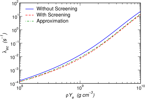
Figure 13: Rate for electron capture on ⁵⁸Fe for a temperature of 7.5 GK as a function of the electron density, $\rho Y_{e}$. The solid line corresponds to the rate computed in ref. [22], the dashed line uses the same matrix elements but includes screening corrections as discussed in the text, see eq. (23). The dashed-dotted line has been obtained using the approximation suggested in equation (26).

A very good approximation can be obtained by using the effective $ft$ value formalism introduced by Fuller et al. [19] which allows accurate interpolations of the tabulated electron capture rates. In this approach an effective $ft$-value is defined that represents an average nuclear matrix element which characterizes the capture rate on a given nucleus:

$$ft_{\rm eff}\equiv\ln 2\frac{F(Q,\mu_{e})}{\lambda_{\rm ec}},$$ (24)

where $\lambda_{\rm ec}$ is the tabulated electron capture rate, $Q$ is the ground-state to ground-state transition energy, and $F$ is the integral

$$F(Q,\mu_{e})=\frac{1}{m_{e}^{5}c^{10}}\int_{\max(Q,m_{e}c^{2})}^{\infty}w^{2}(Q+w)^{2}f(w,\mu_{e},T)dw,$$ (25)

Assuming that the average nuclear matrix element $ft_{\rm eff}$ is unaffected by screening, the ratio of electron capture rates with and without screening is equal to the ratio of $f$ functions, leading to:

$$\lambda_{\rm ec}^{C}=\frac{F(Q+\Delta Q_{C},\mu_{e}-V_{s})}{F(Q,\mu_{e})}\lambda_{\rm ec}$$ (26)

Figure 13 compares the electron capture rate on ⁵⁸Fe computed using the shell-model calculations of [22] with and without screening corrections. In addition, the approximation (26) is also shown. The difference between the exact implementation of screening corrections, eq. (23), and the approximation is never larger than $20\%$ for the conditions shown in figure 13.

References

- [1] H.A. Bethe, Rev. Mod. Phys. 62 (1990) 801.
- [2] S.W. Bruenn, Astrophys. J. Suppl. Ser. 58 (1985) 771.
- [3] S.W. Bruenn, Astrophys. J. 340 (1989) 955; 341 (1989) 385.
- [4] M. Rampp and H.-Th. Janka, Astrophys. J. 539 (2000) L33.
- [5] A. Mezzacappa, M. Liebendörfer, O.E.B. Messer, W.R. Hix, F.-K. Thielemann, and S.W. Bruenn, Phys. Rev. Lett. 86 (2001) 1935.
- [6] M. Liebendörfer, A. Mezzacappa, F.-K. Thielemann, O.E.B. Messer, W.R. Hix, and S.W. Bruenn, Phys. Rev. D 63 (2001) 103004.
- [7] J.R. Wilson, in Numerical Astrophysics, Edited by J.M. Centrella, J.M. LeBlanc and R.L. Bowers (Jones and Bartlett, Boston 1985).
- [8] H.A. Bethe and J.R. Wilson, Astrophys. J. 295 (1985) 14.
- [9] R. Buras, M. Rampp, H.-Th. Janka, and K. Kifonidis, Phys. Rev. Lett. 90 (2003) 241101.
- [10] M. Liebendörfer, M. Rampp, H.-Th. Janka, and A. Mezzacappa, Astrophys. J. 620 (2005) 840.
- [11] R. Buras, H.-Th. Janka, M. Rampp, and K. Kifonidis, Astronom. Astrophys. 447 (2006) 1049; 457 (2006) 281.
- [12] A. Burrows, E. Livne, L. Dessart, C. D. Ott, and J. Murphy, Astrophys. J. 640, (2006) 878 .
- [13] A. Marek and H.-T. Janka, Astrophys. J. 694, (2009) 664 .
- [14] H.-T. Janka, K. Langanke, A. Marek, G. Martínez-Pinedo, and B. Müller, Phys. Rep. 442, (2007) 38.
- [15] S.W. Bruenn, A. Mezzacappa, W.R. Hix, J.M. Blondin, P. Marronetti, O.E.B. Messer, C.J. Dirk, and S. Yoshida, AIP Conf. Proc. 1111 (2009) 593.
- [16] G. M. Fuller, W. A. Fowler, and M. J. Newman, Astrophys. J. Suppl. 42 (1980) 447.
- [17] G. M. Fuller, W. A. Fowler, and M. J. Newman, Astrophys. J. 252 (1982a) 715.
- [18] G. M. Fuller, W. A. Fowler, and M. J. Newman, Astrophys. J. Suppl. 48 (1982b) 279.
- [19] G. M. Fuller, W. A. Fowler, and M. J. Newman, Astrophys. J. 293 (1985) 1.
- [20] E. Caurier, K. Langanke, G. Martínez-Pinedo, and F. Nowacki, Nucl. Phys. A653 (1999) 439.
- [21] K. Langanke and G. Martínez-Pinedo, Nucl. Phys. A673 (2000) 481.
- [22] K. Langanke and G. Martínez-Pinedo, At. Data. Nucl. Data Tables 79 (2001) 1.
- [23] J.M. Sampaio, K. Langanke, G. Martínez-Pinedo, E. Kolbe, and D.J. Dean, Nucl. Phys. A718 (2003) 440c.
- [24] G.H. Lang, C.W. Johnson, S.E. Koonin, and W.E. Ormand, Phys. Rev. C 48 (1993) 1518.
- [25] S.E. Koonin, D.J. Dean, and K. Langanke, Phys. Rep. 278 (1997) 1.
- [26] K. Langanke, E. Kolbe, and D.J. Dean, Phys. Rev. C 63 (2001) 032801.
- [27] A. Heger, K. Langanke, G. Martínez-Pinedo, and S.E. Woosley, Phys. Rev. Lett. 86 (2001) 1678.
- [28] A. Heger, S.E. Woosley, G. Martínez-Pinedo, and K. Langanke, Astrophys. J. 560 (2001) 307.
- [29] A. C. Calder, D. M. Townsley, I. R. Seitenzahl, F. Peng, O. E. B. Messer, N. Vladimirova, E. F. Brown, J. W. Truran, and D. Q. Lamb, Astrophys. J. 656 (2007) 313.
- [30] F. Brachwitz, D. Dean, W. Hix, K. Iwamoto, K. Langanke, G. Martinez-Pinedo, K. Nomoto, M. R. Strayer, and F.-K. Thielemann, Astrophys. J. 536 (2000) 934.
- [31] K. Langanke, G. Martínez-Pinedo, J.M. Sampaio, D.J. Dean, W.R. Hix, O.E.B. Messer, A. Mezzacappa, M. Liebendörfer, H.-Th. Janka, and M. Rampp, Phys. Rev. Lett. 90 (2003) 241102.
- [32] W.R. Hix, O.E.B. Messer, A. Mezzacappa, M. Liebendörfer, J.M. Sampaio, K. Langanke, D.J. Dean, G. Martínez-Pinedo, Phys. Rev. Lett. 91 (2003) 201102.
- [33] G. M. Fuller, Astrophys. J. 252, (1982) 741.
- [34] J. Cooperstein and J. Wambach, Nucl. Phys. A420 (1984) 591.
- [35] N. Paar, G. Colo, E. Khan and D. Vretenar, Phys. Rev. C80 (2009) 055801.
- [36] A.A. Dzhioev, A.I. Vdovin, V.Yu. Ponomarev, J. Wambach, K. Langanke and G. Martinez-Pinedo, Phys. Rev. C81 (2010) 15804.
- [37] K. Langanke, G. Martínez-Pinedo, B. Müller, H.-Th. Janka, A. Marek, W.R. Hix, A. Juodagalvis, and J.M. Sampaio, Phys. Rev. Lett. 100 (2008) 011101.
- [38] A. Juodagalvis, J.M. Sampaio, K. Langanke, and W.R. Hix, Journ. Phys. G: Nucl. Part. Phys. 35 (2008) 014031.
- [39] P. Möller, J.R. Nix, W.D. Myers, and W.J. Swiatecki, At. Data Nucl. Data Tables 59 (1995) 185.
- [40] G. Audi, A.H. Wapstra, and C. Thibault, Nucl. Phys. A729 (2003) 337.
- [41] E. Caurier, G. Martínez-Pinedo, F. Nowacki, A. Poves, A.P. Zuker, Rev. Mod. Phys. 77 (2005) 427.
- [42] I. R. Seitenzahl, D. M. Townsley, F. Peng, and J. W. Truran, At. Data Nuc. Data Tab. 95 (2009) 96.
- [43] S. Gupta, E. F. Brown, H. Schatz, P. Möller, and K. Kratz, Astrophys. J. 662 (2007) 1188.
- [44] D.R. Bes and R.A. Sörensen, Adv. Nucl. Phys. 2 (1969) 129.
- [45] E. Kolbe, K. Langanke, and P. Vogel, Nucl. Phys. A652 (1999) 91.
- [46] K. Langanke, D.J. Dean and W. Nazarewicz, Nucl. Phys. A757 (2005) 360.
- [47] G. Co and S. Krewald, Nucl. Phys. A433 (1985) 351.
- [48] S. Krewald, K. Nakayama and J. Speth, Phys. Rep. 161 (1988) 103.
- [49] E. Kolbe, K. Langanke, and P. Vogel, Phys. Rev. C 62 (2000) 055502.
- [50] N.T. Zinner, K. Langanke, and P. Vogel, Phys. Rev. C 74 (2006) 024326.
- [51] K. Langanke and G. Martínez-Pinedo, Rev. Mod. Phys. 75 (2003) 819.
- [52] W.R. Hix and F.-K. Thielemann, Astrophys. J. 460 (1996) 869.
- [53] W.L. Slattery, G.D. Doolen, and H.E. DeWitt, Phys. Rev. A 26 (1982) 2255.
- [54] S. Ichimaru, Rev. Mod. Phys. 65 (1993) 255.
- [55] D. G. Yakovlev and D. A. Shalybkov, Sov. Sci. Rev. E. Astrophys. Space Phys. 7 (1989) 311.
- [56] T. Rauscher, Astrophys. Jour. Suppl. Ser. 147 (2003) 403.
- [57] F.X. Timmes and F.D. Swesty, Astrophys. J. Suppl. 126 (2000) 501.
- [58] W.R. Hix, A. Mezzacappa, O.E.B. Messer, and S.W. Bruenn, J. Phys. G: Nucl. Part. Phys. 29 (2003) 2523.
- [59] E. Bravo and D. García-Senz, Mon. Not. Roy. Ast. Soc. 307 (1999) 984.
- [60] W. L. Slattery, G. D. Doolen, and H. E. DeWitt, Phys. Rev. A 26 (1982) 2255.
- [61] S. Ichimaru, Rev. Mod. Phys. 65 (1993) 255.
- [62] R. G. Couch and G. L. Loumos, Astrophys. J. 194 (1974) 385.
- [63] N. Itoh, N. Tomizawa, M. Tamamura, S. Wanajo, and S. Nozawa, Astrophys. J. 579 (2002) 380.
- [64] T. Oda, M. Hino, K. Muto, M. Takahara, and K. Sato, At. Data Nucl. Data Tables 56 (1994) 231.
- [65] J.-U. Nabi and H. V. Klapdor-Kleingrothaus, At. Data. Nucl. Data Tables 71 (1999) 149 .
- [66] J. Pruet and G. M. Fuller, Astrophys. J. Suppl. 149 (2003) 189.