The Riemann-Roch Theorem and Zero Energy Solutions of the Dirac Equation on the Riemann Sphere

Abstract

In this paper, we revisit the connection between the Riemann-Roch theorem and the zero energy solutions of the two-dimensional Dirac equation in the presence of a delta-function like magnetic field. Our main result is the resolution of a paradox - the fact that the Riemann-Roch theorem correctly predicts the number of zero energy solutions of the Dirac equation despite counting what seems to be the wrong type of functions.

I Introduction

The cross fertilization between mathematics and physics has proven itself fruitful over the history of science. Often important results in one field generate new ideas in others. For example, the seminal Atiyah-Singer index theorem in mathematics has spawned many novel directions of research in physics due to its connection with the Dirac equation with a background magnetic field. Examples include: string theory, particle theory, condensed matter theory, etc. While solving the Dirac equation with magnetic fields over arbitrary Riemann surfaces is an arduous task, the Riemann-Roch theorem, which counts functions of a particular type (namely, meromorphic functions), correctly predicts the analytic index of the Dirac Hamiltonian. When the magnetic field is sufficiently strong, this index agrees with the multiplicity of the zero energy solution. Therefore it is natural to suspect that the Riemann-Roch theorem can yield information for the $E=0$ eigenfunctions of the solutions to the Dirac equation.

The celebrated Riemann-Roch theoremmiranda deals with functions that are analytic everywhere except a finite set of poles on a closed and compact Riemann surface $X$ (a Riemann surface is a smooth, orientable surface). These functions of interest are known as meromorphic functions. The characteristics of meromorphic functions are summarized by a “divisor” $D=\sum_{p\in X}n_{p}~{}p$, where $\{p\}$ is a finite (and therefore discrete) set of points on $X$ and $n_{p}$ are integers miranda . The vector space $L(D)$ consisting of meromorphic functions that have poles of order $\leq|n_{p}|$ at the points with $n_{p}<0$, and zeros of order $\geq n_{p}$ at for the points with $n_{p}\geq 0$ is the entity of interest. The Riemann-Roch theorem states that $\dim(L(D))-\dim(L(K-D))=\deg(D)+1-g$ with $K$ any “canonical divisor”, $g$ is the genus of $X$ and $\deg(D)=\sum_{p\in X}n_{p}$, the degree of the divisor. The concept of the canonical divisor is irrelevant for the purpose of this paper; this is because for divisors with sufficiently large degree, $\dim(L(K-D))=0$, hence $K$ does not enter. This is the situation we will be focusing on; however for further reading about canonical divisors, we refer the interested reader to Miranda or Hartshornemiranda .

In physics it is known that the Riemann-Roch theorem is connected to the analytical indexatiyah of the two-dimensional Dirac equation under a constant magnetic field pnueli ; iengo . When the total number of flux quantafq is sufficiently big, the latter reduces to the degeneracy of the $E=0$ energy level. In this paper we show that this connection is quite subtle. First of all, meromorphic functions can diverge while the solutionsnote of the Dirac equation in uniform magnetic field do not. This discrepancy can easily be removed by deforming the magnetic field so that

$$B(\vec{r})=\sum_{i}2\pi n_{i}\delta(\vec{r}-\vec{r}_{i})$$ (1)

while maintaining the total magnetic flux. After such deformation it is possible for the $E=0$ solution of the Dirac equation to diverge at a subset of $\{\vec{r}_{i}\}$note2 . The fact that such deformation preserves the analytic index of the Dirac operator is a consequence of the Atiyah-Singer index theorematiyah . However a discrepancy remains even after this deformation, namely, the solutions of the Dirac equation depends on both $z$ and its conjugate $\bar{z}$; these functions are not meromorphic. In this paper we examine and resolve this discrepancy when $X$ is the Riemann sphere. This case is particularly simple because for any divisor $D$ with $\deg(D)\geq 0$ on the Riemann sphere, $\dim(L(K-D))=0$. Moreover, this is the a relevant example to realistic physical systems. Nevertheless, we believe that the idea exposed here can be generalized to other Riemann surfaces with higher genera.

II The Riemann-Roch Problem on the Sphere

For the sake of completeness, in this section the mathematics of the Riemann-Roch problem will be introduced.

II.1 Divisors

In order to assist in the study of meromorphic functions, mathematicians introduce the concept of divisor.

Definition II.1.

A divisor (Fig. 1) is a formal finite linear combination of points of $X$ with integral coefficients. The collection of divisors on a surface $X$, denoted $Div(X)$ form an abelian group with the additive group operation defined as though distinct points were linearly independent vectors. Mathematicians define a partial ordering on $Div(X)$ by defining $D\geq 0$ if all its coefficients are nonnegative.

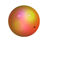
Figure 1: (color on-line) A graphical representation of a divisor. The white and black points denotes poles and zeros resp.

Divisors are of importance in the study of Riemann surfaces because the set of zeros and poles of a meromorphic function on a surface $X$ can be associated to a divisor.

Definition II.2.

Let $f$ be a nonzero meromorphic function on a compact Riemann surface $X$. Then the the divisor of $f$ is defined to be $div(f)=\sum_{p\in X}n_{p}p$ where $n_{p}$ is the order of the zero or pole of $f$ at $p$. By convention, $n_{p}$ is positive when $f$ has a zero at $p$ and negative when $f$ has a pole at $p$. Such divisors are called principal divisors.

It is important to note that such a divisor is always well defined because a meromorphic function on a compact Riemann surface can only have finitely many zeros and polesstein .

Definition II.3.

Let $D$ be a divisor over a Riemann surface $X$, we define a complex vector space $L(D)=\{f{\rm~{}is~{}meromorphic~{}on~{}}X~{}|div(f)+D\geq 0\}$

The dimension of this space is the quantity of interest. While in general, it is very difficult to find the functions in $L(D)$, for the Riemann sphere, we can do so easily.

II.2 L(D) and its Dimension on the Riemann Sphere

First, we preform a stereographic projection to map the Riemann sphere onto $\mathbb{C}_{\infty}:=\mathbb{C}\cup\{\infty\}$, the one-point compactification of the complex plane munkres . Without loss of generality, we may assume that in any divisor $D$, the coefficient associated to the point $\infty$ is $0$. This can be done by appropriately choosing the point from which to stereographically project.

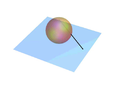
Figure 2: (color on-line) The stereographic projection. The south pole is the base point. A point $P$ on the sphere is projected to the plane by finding the intersection of the line connecting the north pole and $P$ and the plane.

Theorem II.1.

Let $D=\sum_{i=1}^{N}n_{i}p_{i}\in Div({\mathbb{C}_{\infty}})$ and $\deg(D)\geq 0$. Let $f_{D}(z)=\prod_{i=1}^{n}(z-p_{i})^{-n_{i}}$. Then $L(D)=\{g(z)f_{D}(z)|g(z){\rm~{}is~{}a~{}polynomial~{}with~{}}\deg(g)\leq\deg(D)\}$

For those who are not interested in the proof, read corollary II.2 before proceeding to the following section.

Proof.

We will reproduce the proof in Miranda miranda page 149. Let $g(z)$ be a polynomial with degree $d$. Then $div(g)\geq-d~{}\infty$, Hence we have

$$div(f_{D})=\sum_{i}-n_{i}p_{i}+(\sum n_{i})\infty.$$ (2)

Therefore

$$div(g(z)f_{D}(z))+D=div(g)+div(f_{D})+D$$

$$\geq(\sum_{i}n_{i}-d)\infty=(\deg(D)-d)\infty$$ (3)

which is greater than or equal to $0$ if $d\leq\deg(D)$. Thus the space $\{g(z)f_{D}(z)|g(z)$ is a polynomial with $\deg(g)\leq\deg(D)\}$ is a subspace of $L(D)$. Now, for the other inclusion, take any nonzero $h\in L(D)$. Then

$$div(h/f_{D})=div(h)-div(f_{D})$$

$$\geq-D-div(f_{D})=(-\sum_{i}n_{i})\infty=-\deg(D)\infty$$ (4)

which means that $g$ can only have a pole of order at most $\deg(D)$ at $\infty$. Thus $g$ is a polynomial of order at most $\deg(D)$. ∎

It is important to note that in the preceding equations, $\infty$ denotes the antipode of the point projecting to $0$. This point arises because in general as $|z|\rightarrow\infty$, the function $f_{D}(z)$ can have a pole or zero.

Corollary II.2.

Let $D\in Div(\mathbb{C}_{\infty})$ with $\deg(D)\geq 0$. Then $\dim(L(D))=1+\deg(D)$.

Proof.

The set $\{f_{D}(z)...,z^{n}f_{D}(z),...z^{\deg(D)}f_{D}(z)\}$ generates $L(D)$ as a complex vector space, therefore $\dim(L(D))=\deg(D)+1$∎

III The Zero Energy Solutions of the Dirac Equation in a Background Magnetic Field

We will now see the connection between the Riemann-Roch theorem and the Dirac equation. In order to do so, we first introduce the Dirac equation on two dimensional surfacesaharonov . It is a well known result from topology that any two dimensional manifold can be constructed from a planar polygon with edges identified appropriatelymunkres . Therefore, writing the Dirac equation over these surfaces amounts to imposing additional periodic boundary conditions on the corresponding Dirac equation for flat space.

We will use natural units by setting $c=\hbar=1$ as well as fixing the charge $q$ of the particle so Dirac flux quantum $2\pi\hbar/qc=2\pi$.

III.1 The Vector Potential and the Magnetic Field

Let $B(x,y)$ be a magnetic field. We define the vector potential $A_{x}(x,y)$ and $A_{y}(x,y)$ so that

$$\partial_{x}A_{y}(x,y)-\partial_{y}A_{x}(x,y)=B(x,y)$$ (5)

Eq.(5) defines the vector potential up to a gauge transformation. The set of vector potentials which differ from each other by a gauge transformation form an equivalence class and may be considered the same. Choosing a representative of such an equivalence class is known as gauge fixing. In the following, we will fix the gauge by imposing

$$\partial_{x}A_{y}(x,y)+\partial_{y}A_{x}(x,y)=0$$ (6)

It will turn out that this choice of gauge will best exhibit interaction between the Dirac equation and complex geometry.

With the vector potential defined above, the time independent Dirac equation in the presence of a magnetic field becomesjackiw ; aharonov ; pnueli

$$\left(\begin{array}[]{cc}0&-i\partial_{x}-A_{x}-\partial_{y}+iA_{y}\\ -i\partial_{x}-A_{x}+\partial_{y}-iA_{y}&0\end{array}\right)\left(\begin{array}[]{c}u(x,y)\\ v(x,y)\end{array}\right)=E\left(\begin{array}[]{c}u(x,y)\\ v(x,y)\end{array}\right)$$ (7)

III.2 The Magnetic Flux and Divisors

The type of magnetic field given by Eq.(1) admits a natural representation by a divisor, namely

$$D=\sum_{i=1}^{N}n_{i}p_{i}\Leftrightarrow B(\vec{r})=2\pi\sum_{i=1}^{N}n_{i}\delta(\vec{r}-\vec{r}_{p_{i}})$$ (8)

III.3 The Vector Potential as a Complex Function

Note that away from the $\vec{r}_{i}$s, $B(x,y)=0$. Therefore, we have

$$\partial_{x}A_{y}-\partial_{y}A_{x}=0$$

$$\partial_{x}A_{x}+\partial_{y}A_{y}=0$$ (9)

Let us define

$$F(z,\bar{z})=A_{y}(x,y)+iA_{x}(x,y)$$ (10)

Then Eq.(9) becomes $\partial_{\bar{z}}F(z,\bar{z})=0$, the Cauchy-Riemann condition on $F(z,\bar{z})$. As usual, $\partial_{z}=(\partial_{x}-i\partial_{y})/2$, and $\partial_{\bar{z}}=(\partial_{x}+i\partial_{y})/2$. Moreover, by the Stokes theorem, the equation $\partial_{x}A_{y}-\partial_{y}A_{x}=2\pi\sum_{i}n_{i}\delta(\vec{r}-\vec{r}_{i})$ rewrites into the integral form

$$\oint_{C_{i}}\vec{A}(x,y)\cdot d\vec{r}=2\pi n_{i}$$ (11)

where $C_{i}$ is a counter-clockwise loop enclosing only the $i$-th magnetic flux point (Fig. 3)

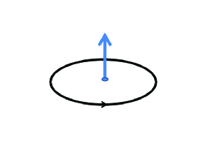
Figure 3: (color online) As dictated by the Stokes theorem, the loop integral of the vector potential is equal to the magnetic flux.

This integral equation translates into

$$\oint_{C_{i}}F(z)dz=2\pi in_{i}$$ (12)

Now, by the Cauchy residue theoremstein ; miranda , we can represent $F(z)$ as

$$F(z)=\sum_{i=1}^{N}\frac{n_{i}}{z-z_{i}}$$ (13)

where $z_{i}$ represents the position of the $i$-th magnetic flux point. The reader might have noticed that a holomorphic function $G(z)$ could be added to $F(z)$ while still preserving the integral. Ignoring the holomorphic part of $G(z)$ amounts to a further fixing of gauge.

III.4 The Dirac Equation in Complex Coordinates

We first make the following standard definitions:

$$A_{z}=\frac{1}{2}(A_{x}-iA_{y})$$

$$A_{\bar{z}}=\frac{1}{2}(A_{x}+iA_{y})$$ (14)

Using $z$ and $\bar{z}$ as coordinates, the Dirac equation in the presence of a magnetic field reads

$$2i\left(\begin{array}[]{cc}0&\partial_{z}-iA_{z}\\ \partial_{\bar{z}}-iA_{\bar{z}}&0\end{array}\right)\left(\begin{array}[]{c}u(z,\bar{z})\\ v(z,\bar{z})\end{array}\right)=E\left(\begin{array}[]{c}u(z,\bar{z})\\ v(z,\bar{z})\end{array}\right)$$ (15)

Taking $E=0$, Eq.(15) becomes:

$$(\partial_{\bar{z}}-iA_{\bar{z}})u(z,\bar{z})=0$$

$$(\partial_{z}-iA_{z})v(z,\bar{z})=0$$ (16)

Substituting in Eq.(10), these two equations become

$$(\partial_{\bar{z}}+\frac{1}{2}\bar{F}(z))u(z,\bar{z})=0$$

$$(\partial_{z}-\frac{1}{2}F(z))v(z,\bar{z})=0$$ (17)

III.5 Solving the Dirac Equation

The second line of Eq.(9) ensures that it is possible to pick a $\Phi(x,y)$ so that

$$A_{x}=-\partial_{y}\Phi~{}~{}A_{y}=\partial_{x}\Phi,$$ (18)

or equivalently, $A_{z}=-i\partial_{z}\Phi/2$ and $A_{\bar{z}}=i\partial_{\bar{z}}\Phi/2$. Since $A_{z}=-iF/2$ and $A_{\bar{z}}=i\bar{F}/2$, this means

$${1\over 2}\sum_{i=1}^{N}\frac{n_{i}}{\bar{z}-\bar{z}_{i}}=\frac{1}{2}\bar{F}(z)=\partial_{\bar{z}}\Phi$$

$${1\over 2}\sum_{i=1}^{N}\frac{n_{i}}{z-z_{i}}=\frac{1}{2}F(z)=\partial_{z}\Phi$$ (19)

In writing down the above equations we have used Eq.(10).

A simple calculation shows that

$$\Phi(z,\bar{z})=\sum_{i=1}^{N}\log\left(|z-z_{i}|^{n_{i}}\right)$$ (20)

satisfies the above equations. Substituting $\Phi$ into the Dirac equation allows us to write the two differential equations as

$$(\partial_{\bar{z}}+\partial_{\bar{z}}\Phi(z,\bar{z}))u(z,\bar{z})=0$$

$$(\partial_{z}-\partial_{z}\Phi(z,\bar{z}))v(z,\bar{z})=0$$ (21)

Solving this equation by separation of variables gives the solutions

$$u(z,\bar{z})=f(z)e^{-\Phi(z,\bar{z})}$$

$$v(z,\bar{z})=g(\bar{z})e^{\Phi(z,\bar{z})}$$ (22)

Notice that the functions $f(z)$ and $g(\bar{z})$ do not contribute to differentiation with respect to $\bar{z}$ and $z$ respectively. Substituting in $\Phi(z,\bar{z})$ gives

$$u(z,\bar{z})=f(z)\prod_{i=1}^{N}\frac{1}{|z-z_{i}|^{n_{i}}}$$

$$v(z,\bar{z})=g(\bar{z})\prod_{i=1}^{N}|z-z_{i}|^{n_{i}}$$ (23)

Because our original divisor does not specify any poles or zeroes at $\infty$, $v(z,\bar{z})$ is not a valid solution because it diverges as $|z|\rightarrow\infty$. Now in order for $u$ to remain bounded at infinity, $f(z)$ must be a polynomial satisfying $\deg(f(z))\leq\sum_{i}n_{i}$. The reason that $f(z)$ cannot be a rational function of the form, say $1/z^{m}$, is because it makes the divisor smaller under the partial ordering of $Div(X)$ (see “Divisors”). Thus we conclude that there are $1+\sum_{i}n_{i}$ linearly independent solutions obtained by setting $f(z)$ equal to $1,z,z^{2}...z^{1+\sum_{i}n_{i}}$. Notice that $1+\sum_{i}n_{i}=\deg(D)+1$, a number which we calculated to be the complex dimension of $L(D)$ from a purely mathematical viewpoint in the previous sections.

Despite the above success, the function $u(z,\bar{z})$ in Eq.(23) is not meromorphic hence is not a member of $L(D)$. Another equivalent statement is that Eq.(21) is not the Cauchy-Riemann equation $\partial_{\bar{z}}u=0$. We will remedy this situation with the use of a phase transformation.

IV The phase Transformation

Our objective now is to transform functions $u(z,\bar{z})=f(z)\prod_{i=1}^{N}\frac{1}{|z-z_{i}|^{n_{i}}}$ into meromorphic functions. This can be done by multiplying $u$ by the unit modulus complex valued function $\chi(z,\bar{z})=\prod_{i=1}^{N}(\frac{\bar{z}-\bar{z}_{i}}{z-z_{i}})^{n_{i}/2}$. By taking the product $\chi u$, we get the meromorphic function

$$\chi(z,\bar{z})u(z,\bar{z})=f(z)\prod_{i=1}^{N}\frac{1}{(z-z_{i})^{n_{i}}}.$$ (24)

Where $f(z)=1,z,...,z^{\sum n_{i}}$. Notice that this gives exactly the space $L(D)$ of Theorem 2.1.

IV.1 Monodromy

We now show $\chi$ is single valued. It is in fact a nontrivial result that $\chi$ does not have any branches. Because $\chi$ has unit modulus, we can write it as $e^{i\theta(z,\bar{z})}$. After doing so, it suffices to study the behavior of this function along a loop around any one of the $z_{k}$.

Theorem IV.1.

As $\chi(z,\bar{z})$ wraps once around any one of the $z_{k}$, $\theta(z,\bar{z})$ changes by $-2\pi n_{k}$ (an example is shown in Fig.4).

Proof.

First it is clear that if the loop encloses only $z_{k}$, the only factor in $\chi$ that will exhibit winding is $(\frac{\bar{z}-\bar{z}_{k}}{z-z_{k}})^{n_{k}/2}$. Now, we have

$$\bar{z}-\bar{z}_{k}=|z-z_{k}|e^{i\arg(z-z_{k})}$$

$$z-z_{k}=|z-z_{k}|e^{-i\arg(z-z_{k})}$$ (25)

Therefore, we have

$$\left(\frac{\bar{z}-\bar{z}_{k}}{z-z_{k}}\right)^{n_{k}/2}=e^{-in_{k}\arg(z-z_{k})}$$ (26)

Now clearly as $z$ wraps around $z_{k}$ once counterclockwise, the exponent of the right hand side changes by $-2\pi n_{k}$∎

Now we can demonstrate that this phase transformation is single valued.

Corollary IV.2.

$\chi(z,\bar{z})$ has no branches.

Proof.

After a full loop $\Delta\theta=-2\pi n_{k}$, so $e^{i\Delta\theta}=1$ thus after a loop, the value of $\chi(z,\bar{z})$ remains the same. ∎

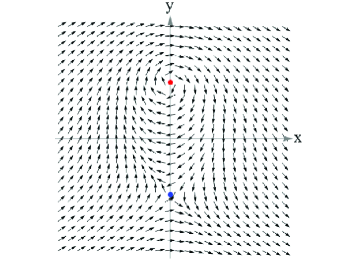
Figure 4: (color on-line) A plot of the real and imaginary parts of $\chi(z,\bar{z})$ as a vector field.The $n_{k}$ associated with the red/blue points are $\pm 1$.

IV.2 Recovery of Cauchy-Riemann Equations from the Dirac Equation

We will now show that the transformation of $u(z,\bar{z})$ into a meromorphic function is not a coincidence. It results from the fact that the Dirac equation transforms into the Cauchy-Riemann equations after the phase transformation.

Theorem IV.3.

The equation $(\partial_{\bar{z}}+\partial_{\bar{z}}\Phi)u=0$ transforms into $\partial_{\bar{z}}(\chi u)=0$.

Proof.

Let $\zeta(z)=\chi(z,\bar{z})u(z,\bar{z})$. Then $u=\chi^{-1}\zeta=\bar{\chi}\zeta$. We have

$$\partial_{\bar{z}}u=\partial_{\bar{z}}(\bar{\chi}\zeta)=\zeta\partial_{\bar{z}}\bar{\chi}+\bar{\chi}\partial_{\bar{z}}\zeta$$ (27)

By an elementary computation $\chi\partial_{\bar{z}}\bar{\chi}=-\partial_{\bar{z}}\Phi$. As a result, the Dirac equation becomes

$$\zeta\partial_{\bar{z}}\bar{\chi}+\bar{\chi}\partial_{\bar{z}}\zeta+(\partial_{\bar{z}}\Phi)(\bar{\chi}\zeta)=0$$ (28)

Now we can write

$$\zeta\partial_{\bar{z}}\bar{\chi}=\zeta\bar{\chi}\chi\partial_{\bar{z}}\bar{\chi}=-\partial_{\bar{z}}\Phi(\zeta\bar{\chi})$$ (29)

This cancels the extraneous $\partial_{\bar{z}}\Phi(\zeta\bar{\chi})$ in the previous equation giving us the Cauchy-Riemann equation. ∎

V Conclusion

On the Riemann sphere, we have shown that upon a phase transformation the zero energy solutions of the Dirac equation in the presence of a magnetic field given by Eq.(1) becomes the meromorphic functions of the Riemann-Roch theorem. We have also performed the analogous calculation for the complex torus in which there is a periodic boundary condition requiring us to represent the vector potential in terms of the elliptic theta functionmiranda . In this case, the phase transformation is replaced by the ratio of elliptic theta functions.

In general, for Riemann surfaces of higher genera, it is not clear that such phase transformations exist. This is because the phase transformation must be consistent with the appropriate periodic boundary conditions discussed earlier. A related fact is that it is difficult to prove the existence of nonconstant meromorphic functions on arbitrary compact Riemann surfaces; this was first demonstrated by Riemannmiranda . We conjecture that the existence of a phase transformation is equivalent to the existence of nonconstant meromorphic functions. If this is true, there might be an alternative proof for the fact that compact Riemann surfaces are “projective algebraic”miranda .

Acknowledgements I thank Prof. Dung-Hai Lee of the University of California Berkeley for explaining the Dirac equation and its solutions to me. In addition, I thank Prof. Wu-Yi Hsiang of the University of California Berkeley for general discussions about mathematics. I also am grateful to Prof. R. Jackiw for pointing out relevant references.

References

- (1) See, e.g., Miranda, R. Algebraic Curves and Riemann Surfaces. Providence, RI.: American Mathematical Society, 1995; Hartshorne, R. Algebraic Geometry (Graduate Texts in Mathematics). New York: Springer, 1997. page 441.
- (2) Atiyah, M. F. and Singer, I. M. Annals of Math. 87, 484 (1968).
- (3) Aharonov, Y. and Casher, A. Phys. Rev. A 19, 2461 (1979).
- (4) Jackiw, R. Phys. Rev. D 29 2375 (1984); Jackiw, R. Phys. Rev. D 33 2500 (1986).
- (5) Pnueli, A. J. Phys. A: Math. Gen. 27 1345 (1994).
- (6) Iengo, R. and Li, D. P. Nucl. Phys. B. 413 735 (1994).
- (7) The number of flux quanta is defined as where is the total flux passing through the Riemann surface and is the Dirac flux quantum. We shall choose the natural unit and fix the charge of the particle so that .
- (8) In the rest of this paper the phrase ”solutions of the Dirac equation” is used to denote the solutions of the time-independent Dirac equation in the presence of magnetic field.
- (9) The reader might wonder if deforming the magnetc flux to make divergent solutions spoils square integrability. The fact is that the Dirac equation always is a low energy effective theory, hence has a short-distance cutoff. This cutoff rounds off the divergence.
- (10) Stein, E. M. and Shakarchi R. Complex Analysis (Princeton Lectures in Analysis). New York: Princeton UP, 2003.
- (11) Munkres, J. R. Topology. Upper Saddle River, NJ: Prentice Hall, Inc., 2000.