Quantum Stackelberg duopoly in the presence of correlated noise

Abstract

We study the influence of entanglement and correlated noise using correlated amplitude damping, depolarizing and phase damping channels on the quantum Stackelberg duopoly. Our investigations show that under the action of amplitude damping channel a critical point exists for unentangled initial state as well, at which firms get equal payoffs. The game becomes a follower advantage game when the channel is highly decohered. Two critical points corresponding to two values of the entanglement angle are found in the presence of correlated noise. Within the range of these limits of entanglement angle, the game is follower advantage game. In case of depolarizing channel, the payoffs of the two firms are strongly influenced by the memory parameter. The presence of quantum memory ensures the existence of Nash equilibrium for the entire range of decoherence and entanglement parameters for both the channels. A local maximum in the payoffs is observed which vanishes as the channel correlation increases. Moreover, under the influence of depolarizing channel, the game is always a leader advantage game. Furthermore, it is seen that phase damping channel does not effect the outcome of the game.
PACS: 02.50.Le, 03.67.-a, 05.30.-d.
Keywords: Quantum channels; correlated noise; Stackelberg duopoly.

1 Introduction

Game theory is the mathematical study of interaction among independent, self interested agents. It emerged from the work of Von Neumann [1], and is now used in various disciplines like economics, biology, medical sciences, social sciences and physics [2, 3]. Due to dramatic development in quantum information theory [4], the game theorists [$5$-$12$] have made strenuous efforts to extend the classical game theory into the quantum domain. The first attempt in this direction was made by Meyer [13] by quantizing a simple coin tossing game. Applications of quantum games are reviewed by several authors [$14$-$18$]. A formulation of quantum game theory based on the Schmidt decomposition is presented by Ichikawa et al. [19]. Recently, Xia et al. [20, 21] have investigated the quantum Stackelberg duopoly game under the influence of decoherence and have found a critical point for the maximally entangled initial state against the damping parameter for the amplitude damping environment under certain conditions.

In practice no system can be fully isolated from its environment. The interaction between system and environment leads to the destruction of quantum coherence of the system. It produces an inevitable noise and results in the loss of information encoded in the system [22]. This gives rise to the phenomenon of decoherence. Quantum information are encoded in qubits during its transmission from one party to another and require communication channels. In a realistic situation, the qubits have a nontrivial dynamics during transmission because of their interaction with the environment. Therefore, a party may receive a set of distorted qubits because of the disturbing action of the channel. Studies on quantum channels have attracted a lot of attention in recent past [23, 24]. Early work in this direction was devoted mainly to memoryless channels for which consecutive signal transmissions through the channel were not correlated. In the correlated channels (i.e. the channels with memory), the noise acts on consecutive uses of the channel. The effect of decoherence and correlated noise in quantum games have produced interesting results and is studied by number of authors  [$23$-$28$].

In this paper, we study the effect of correlated noise introduced through amplitude damping, phase damping and depolarizing channels parameterized by the decoherence parameters $p_{1}$ and $p_{2}$ and the memory parameters $\mu_{1}$ and $\mu_{2}$, on the quantum Stackelberg duopoly game. The decoherence parameters $p_{i}$ and the memory parameters $\mu_{i}$ range from $0$ to $1$. The lower and upper limits of decoherence parameter $p_{i}$ correspond to the undecohered and fully decohered cases, respectively. Whereas the lower and upper limits of memory parameter $\mu_{i}$ correspond to the uncorrelated and fully correlated cases, respectively. It is seen that there exists a critical point in the case of amplitude damping channel for initially unentangled state at which both firms have equal payoffs. The game transforms from leader advantage to the follower advantage game beyond this point, for highly decohered case in the presence of memory. For initially entangled state under the influence of amplitude damping channel we found two critical points. The game behaves as a follower advantage game within these two critical points. In the case of depolarizing channel the high correlation results in high payoffs. However, phase damping channel has no effect on the game dynamics.

2 Stackelberg duopoly game

Stackelberg duopoly is a market game, which is rather different from the Cournot duopoly game. In Cournot duopoly game, two firms simultaneously provide a homogeneous product to the market and guess that what action the opponent will take. However Stackelberg duopoly is a dynamic model of duopoly game in which one firm, say firm $A$ moves first and the other firm, say $B$, goes after. Before making its decision, firm $B$ observes the move of firm $A$. This transforms the static nature of Cournot duopoly game to a dynamic one. Firm $A$ is usually called the leader and firm $B$ the follower, on this basis the game is also called the leader-follower model [30]. In classical Stackelberg duopoly it is assumed that firm $B$ will respond optimally to the strategic decision of firm $A$. As firm $A$ can precisely predict firm $B$’s strategic decision, firm $A$ chooses its move in such a way that maximizes its own payoff. This informational asymmetry makes the Stackelberg duopoly as the first mover advantage game.

A number of authors have proposed various quantization protocols for observing the behavior of Stackelberg duopoly game in the quantum realm [9,29-32]. It has been shown that quantum entanglement affects payoff of the first mover and produces an equilibrium that corresponds to classical static form of the same game [33]. The effects of decoherence produced by various prototype quantum channels on quantum Stackelberg duopoly have been studied by Zhu et al. [20]. We study the effects of correlated noise on quantum Stackelberg duopoly, using amplitude damping, phase damping and depolarizing channels.

3 Calculations

In a quantum Stackelberg duopoly game, for each firm $A$ and $B$ the game space is a two dimensional complex Hilbert space of basis vectors $|0\rangle$ and $|1\rangle$, that is, the game consists of two qubits, one for each firm. We consider that the initial state of the game is given by

$$|\psi_{i}\rangle=\cos\theta|00\rangle+\sin\theta|11\rangle$$ (1)

where $\theta$ is a measure of entanglement. The state is maximally entangled at $\theta=\frac{\pi}{4}$. In the presence of noise the evolution of an arbitrary system can be described in terms of Kraus operators as [4]

$$\rho=\sum\limits_{l}E_{l}\rho_{i}E_{l}^{{\dagger}}$$ (2)

where $\rho_{i}=|\psi_{i}\rangle\langle\psi_{i}|$ is the initial density matrix and the Kraus operators $E_{l}$ satisfy the following completeness relation

$$\sum\limits_{l}E_{l}^{{\dagger}}E_{l}=1$$ (3)

The single qubit Kraus operators for uncorrelated quantum amplitude damping channel are given as [23, 24]

$$E_{0}=\left(\begin{array}[]{cc}1&0\\ 0&\sqrt{1-p}\end{array}\right),\mathrm{\qquad}E_{1}=\left(\begin{array}[]{cc}0&\sqrt{p}\\ 0&0\end{array}\right)$$ (4)

The Kraus operators for amplitude damping channel with correlated noise for a two qubit system are given as [24]

$$E_{00}^{c}=\left(\begin{array}[]{cccc}\sqrt{1-p}&0&0&0\\ 0&1&0&0\\ 0&0&1&0\\ 0&0&0&1\end{array}\right),\mathrm{\qquad}E_{11}^{c}=\left(\begin{array}[]{cccc}0&0&0&0\\ 0&0&0&0\\ 0&0&0&0\\ \sqrt{p}&0&0&0\end{array}\right)$$ (5)

The action of such a channel on the the initial density matrix  of the system is given by

$$\rho=\left(1-\mu\right)\sum\limits_{m,n=0}^{1}E_{mn}^{u}\,\rho_{i}\,E_{mn}^{u{\dagger}}+\mu\sum\limits_{l=0}^{1}E_{ll}^{c}\,\rho_{i}\,E_{ll}^{c{\dagger}}$$ (6)

where the superscripts $u$ and $c$ represent the uncorrelated and correlated parts of the channel, respectively. The above relation means that with probability $\mu$ the noise is correlated and with probability $\left(1-\mu\right)$ it is uncorrelated. The Kraus operators for phase damping channel with uncorrelated noise for a system of two qubits are given as [23, 24]

$$E_{mn}^{u}=\sqrt{e_{m}e_{n}}\sigma_{m}\otimes\sigma_{n},\hskip 36.135ptm,n=0,\mathrm{{\ }3}$$ (7)

whereas the one with correlated noise are given as

$$E_{ll}^{c}=\sqrt{e_{l}}\sigma_{l}\otimes\sigma_{l},\mathrm{{\hskip 36.135pt}l=0,{\ }3}$$ (8)

Similarly, the Kraus operators for depolarizing channel are described by equations (7) and (8) with indices run from $0$ to $3$. Where $\sigma_{0}$ is identity operator for a single qubit and $\sigma_{1},\sigma_{2}$ and $\sigma_{3}$ are the Pauli spin operators. For phase damping channel, $e_{0}=\left(1-p_{i}\right)$ and $e_{3}=p_{i}$ and for depolarizing channel $e_{0}=\left(1-p_{i}\right)$, $e_{1}=e_{2}=e_{3}=\frac{1}{3}p_{i}$, where $p_{i}$ correspond to the decoherence parameters of the first and second use of the channel. The action of such a channel on the quantum system can be defined in a similar fashion as described earlier in equation (6).

In quantum Stackelberg duopoly game each firm has two possible strategies $I$, the identity operator and $C$, the inversion operator or Pauli’s bit-flip operator. Let $x$ and $1-x$ stand for the probabilities of $I$ and $C$ that firm $A$ applies and $y$, $1-y$, are the probabilities that firm $B$ applies, respectively. The final state after the action of the channel is given by [32]

$$\rho_{f} = xyI_{A}\otimes I_{B}\ \rho\ I_{A}^{{\dagger}}\otimes I_{B}^{{\dagger}}+x\left(1-y\right)I_{A}\otimes C_{B}\ \rho\ I_{A}^{{\dagger}}\otimes C_{B}^{{\dagger}}$$ (9)

$$+y\left(1-x\right)C_{A}\otimes I_{B}\ \rho\ C_{A}^{{\dagger}}\otimes I_{B}^{{\dagger}}$$

$$+\left(1-x\right)\left(1-y\right)C_{A}\otimes C_{B}\ \rho\ C_{A}^{{\dagger}}\otimes C_{B}^{{\dagger}}$$

where $\rho$ (equation (6)) is the density matrix of the game after the channel action.

Suppose that the player’s moves in the quantum Stackelberg duopoly are given by probabilities lying in the range $[0,1]$. In classical duopoly game the moves of firms $A$ and $B$ are given by quantities $q_{1}$ and $q_{2}$, which have values in the range $[0,\infty)$. We assume that firms $A$ and $B$ agree on a function that uniquely defines a real positive number in the range $(0,1]$ for every quantity $q_{1}$, $q_{2}$ in $[0,\infty)$. Such a function is given by $1/(1+q_{i})$, so that firms $A$ and $B$ find $x$ and $y$, respectively, as

$$x=\frac{1}{1+q_{1}}\mathrm{,\qquad}y=\frac{1}{1+q_{2}}$$ (10)

The payoffs of firms $A$ and $B$ are given by the following trace operations

$$P_{A}\left(q_{1},q_{2}\right)=\mathrm{Tr}\left[\rho_{f}P_{A}^{\mathrm{op}}\left(q_{1},q_{2}\right)\right]\mathrm{,\qquad}P_{B}\left(q_{1},q_{2}\right)=\mathrm{Tr}\left[\rho_{f}P_{B}^{\mathrm{op}}\left(q_{1},q_{2}\right)\right]$$ (11)

where $P_{A}^{\mathrm{op}}$, $P_{B}^{\mathrm{op}}$ are payoff operators of the firms and are given by

$$P_{A}^{\mathrm{op}}\left(q_{1},q_{2}\right) = \frac{q_{1}}{q_{12}}\left(k\rho_{11}-\rho_{22}-\rho_{33}\right)$$

$$P_{B}^{\mathrm{op}}\left(q_{1},q_{2}\right) = \frac{q_{2}}{q_{12}}\left(k\rho_{11}-\rho_{22}-\rho_{33}\right)$$ (12)

where $\rho_{ii}$ are the diagonal elements of the final density matrix, $k$ is a constant as given in ref. [30] and $q_{12}$ is given by

$$q_{12}=\frac{1}{\left(1+q_{1}\right)\left(1+q_{2}\right)}$$ (13)

The backward-induction outcome in the Stackelberg duopoly is found by first finding the reaction $R_{2}\left(q_{1}\right)$ of firm $B$ to an arbitrary quantity $q_{1}$ chosen by firm $A$. It is found by differentiating firm $B$’s payoff with respect to $q_{2}$, and maximizing the result for $q_{1}$ and can be written as

$$R_{2}\left(q_{1}\right)=\max P_{B}\left(q_{1},q_{2}\right)$$ (14)

Once firm $B$ chooses this quantity, firm $A$ can compute its optimization problem by differentiating its own payoff with respect to $q_{1}$and then maximizing it to find the value $q_{1}=q_{1}^{\ast}$. Using the value of $q_{1}^{\ast}$ in equation (14) we can get the value of $q_{2}^{\ast}$. These quantities define the backward-induction outcome of quantum Stackelberg duopoly game and represent the subgame perfect Nash equilibrium point. The payoffs of the firms at this point can be found using equation (11).

4 Results and discussion

We suppose that before the firms measure their payoffs the game evolves twice through different quantum correlated channels. That is, the state, prior and after the firms apply their operators, is influenced by the correlated noisy channels.

4.1 Correlated amplitude damping channel

The subgame perfect Nash equilibrium point for the game under the influence of correlated quantum amplitude damping channel becomes

$$q_{1}^{\ast} = \frac{-k\cos^{2}\theta+A_{1}\left(p_{1},p_{2},\mu_{1},\mu_{2}\right)}{-4+A_{2}\left(p_{1},p_{2},\mu_{1},\mu_{2}\right)}$$

$$q_{2}^{\ast} = \frac{\frac{1}{4}k\cos^{2}\theta-B_{1}\left(p_{1},p_{2},\mu_{1},\mu_{2}\right)}{16+B_{2}\left(p_{1},p_{2},\mu_{1},\mu_{2}\right)}$$ (15)

where the damping function $A_{i}$ and $B_{i}$ are given in appendix A.

If we consider the influence of decoherence in the second evolution only ($p_{1}=0$), equation (15) for unentangled initial state reduces to the following form

$$q_{1}^{\ast} = \frac{1}{2-4p_{2}(1-\mu_{2})}$$

$$q_{2}^{\ast} = \frac{1-2p_{2}(1-\mu_{2})}{2[2-p_{2}\{6-5\mu_{2}-p_{2}(1-\mu_{2})(5-8\mu_{2})\}]}$$ (16)

Here we have taken $k=1$. The firms’ payoffs under this situation become

$$P_{A} = \frac{1}{8-16p_{2}(1-\mu_{2})}$$

$$P_{B} = \frac{1-2p_{2}(1-\mu_{2})}{8\{2-p_{2}(6-5\mu_{2})+p_{2}^{2}(8\mu_{2}+5)(\mu_{2}-1)\}}$$ (17)

In the classical form of the duopoly the perfect game Nash equilibrium is a point, whereas in this case it is a function of both decoherence and memory parameters. It can be easily seen that the results of ref. [20] are retrieved by setting $\mu_{2}=0$, and setting $p_{2}=0$ reproduces the results of classical game. The existence of Nash equilibrium requires that firms’ moves ($q_{1}^{\ast}$ and $q_{2}^{\ast}$) should have positive values. It can easily be checked using equation (16) that in the absence of quantum memory, no Nash equilibrium exists for $p_{2}>\frac{1}{2}$. The presence of quantum memory allows the existence of Nash equilibrium for the entire range of values of $p_{2}$, when $\mu_{2}\geq 0.85$.

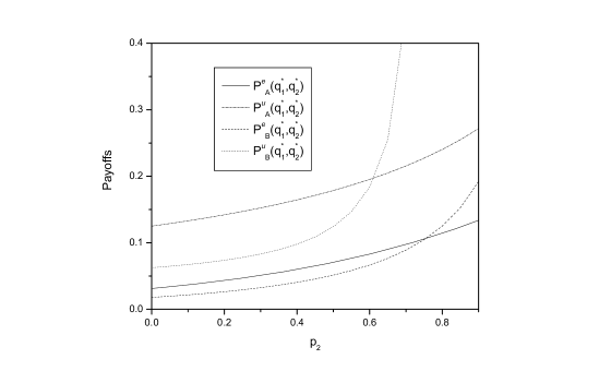
\put(-350.0,220.0){}

Figure 1: The payoffs ($P_{A}(q_{1}^{\ast},q_{2}^{\ast})$ and $P_{B}(q_{1}^{\ast},q_{2}^{\ast})$) are plotted at the subgame perfect Nash equilibrium point against the decoherence parameter $p_{2}$ both for entangled and unentangled initial states under the action of amplitude damping channel, with values of other parameters $k=1$ and $p_{1}=\mu_{1}=0$. For maximally entangled initial state the memory parameter $\mu_{2}=0.9$, and for unentangled initial state $\mu_{2}=0.7$

To see the influence of decoherence and quantum memory on firms’ payoffs at the subgame perfect Nash equilibrium, we plot the payoffs (equation (17)) in figure $1$ as a function of decoherence parameter $p_{2}$. In the figure the dotted and dashed-dotted lines represent firm $A$ and firm $B$ payoffs for unentangled initial state, respectively. The superscripts $u$ and $e$ of $P_{A}$ ($P_{B}$) in the figure stand for unentangled and entangled initial states respectively. It can be seen from the figure that a critical point exists due to the presence of memory at which both firms are equally benefited. This situation has not been observed, in the absence of memory, for unentangled initial state of the game. That is, in the absence of quantum memory the game is always first mover advantage game. For highly decohered channel and $\mu<1$, a transition from first mover advantage into second mover advantage occurs in the game behavior. It can also be seen from equation (17) that for fully correlated and fully decohered channel, both firms are equally benefited and get a payoff equal to $\frac{1}{8}$. It can also be shown that for smaller values of decoherence, the game is always first mover advantage irrespective of the value of the quantum memory.

For a maximally entangled initial state of the game, the subgame perfect Nash equilibrium point becomes

$$q_{1}^{\ast} = \frac{1-3p_{2}^{2}(-1+\mu_{2})-p_{2}(2-3\mu_{2})}{4-8p_{2}(1-\mu_{2})}$$

$$q_{2}^{\ast} = \frac{\begin{array}[]{c}[[-1+p_{2}\{2+3p_{2}(-1+\mu_{2})-3\mu_{2}\}]\\ \times\{1+2p_{2}(-1+\mu_{2})\}]\end{array}}{\begin{array}[]{c}[-7+p_{2}(28-26\mu_{2})+9p_{2}^{4}(-1+\mu_{2})^{2}+p_{2}^{2}\\ \times(-22+46\mu_{2}-23\mu_{2}^{2})-6p_{2}^{3}(2-5\mu_{2}+3\mu_{2}^{2})]\end{array}}$$ (22)

The firms’ payoffs corresponding to these values of $q_{i}^{\ast}$ become

$$P_{A} = \frac{\{-1+p_{2}(2-3\mu_{2})+3p_{2}^{2}(-1+\mu_{2})\}^{2}}{32(1+2p_{2}(-1+\mu_{2}))}$$

$$P_{B} = \frac{\begin{array}[]{c}[-\{1+2p_{2}(-1+\mu_{2})\}\{-1+p_{2}(2-3\mu_{2})\\ +3p_{2}^{2}(-1+\mu_{2})\}^{2}]\end{array}}{\begin{array}[]{c}[8\{-7+p_{2}(28-26\mu_{2})+9p_{2}^{4}(-1+\mu_{2})^{2}\\ +p_{2}^{2}(-22+46\mu_{2}-23\mu_{2}^{2})-6p_{2}^{3}(2-5\mu_{2}+3\mu_{2}^{2})\}]\end{array}}$$ (27)

One can easily check that these results reduce to the results of refs. [20, 33] by setting $\mu_{2}=0$ and $p_{2}=0$ respectively. The payoffs of firms for the maximally entangled initial state are plotted as function of decoherence parameter $p_{2}$ in figure $1$. The solid line represents firm $A$ payoff and the dashed line represents firm $B$ payoff for maximally entangled initial state. One can easily check that for a maximally entangled initial state, the presence of quantum memory makes the firms better off as compared to the uncorrelated case of the channel. Furthermore, quantum memory shifts the critical point to higher payoffs than the critical point for maximally entangled initial state when the channel is uncorrelated. This can also be shown that for a given decoherence level, the firms become worse off and the game becomes a follower advantage as the channel becomes more correlated.

\put(-350.0,220.0){}

Figure 2: The payoffs of the two firms are plotted at the subgame perfect Nash equilibrium point against the entanglement angle $\theta$ under the action of amplitude damping channel, with other parameters $p_{1}=p_{2}=0.5$, $k=1$ and $\mu_{1}=\mu_{2}=0.5$.

The effect of entanglement in the initial state on the firms’ payoffs is shown in figure $2$. Here we have taken into account the two decohering correlated processes. It can be checked that for certain range of decoherence parameters, in the absence of quantum memory, the moves of firms are negative. This means that no Nash equilibrium exists in the region of these values of decoherence parameters. The presence of quantum memory, however, resolves this problem. As can be seen from figure $2$, the presence of quantum memory in the payoff functions results into two critical points corresponding to two different values of entanglement parameter. The game is a follower advantage in this range of entanglement angle. The leader firm is worse off in this range of values of $\theta$ and a global minimum in payoffs occurs at $\theta=\frac{\pi}{2}$.

4.2 Correlated Depolarizing channel

When the game evolves under the influence of correlated depolarizing channel, the moves of firms at subgame perfect Nash equilibrium point become

$$q_{1}^{\ast} = \frac{81k\cos^{2}\theta+A_{1}^{\prime}\left(p_{1},p_{2},\mu_{1},\mu_{2}\right)}{3244+A_{2}^{\prime}\left(p_{1},p_{2},\mu_{1},\mu_{2}\right)}$$

$$q_{2}^{\ast} = \frac{6561k\cos^{2}\theta+B_{1}^{\prime}\left(p_{1},p_{2},\mu_{1},\mu_{2}\right)}{52488+B_{2}^{\prime}\left(p_{1},p_{2},\mu_{1},\mu_{2}\right)}$$ (28)

where the damping parameters $A_{1}^{\prime},A_{2}^{\prime},B_{1}^{\prime}$ and $B_{2}^{\prime}$ are given in appendix A. For unentangled initial state, firms’ payoffs at the subgame perfect Nash equilibrium point become

$$P_{A} = -\frac{(3-2p_{2})^{2}\{1+2p_{2}(-1+\mu_{2})\}^{2}}{24\{-3-6p_{2}(-1+\mu_{2})+4p_{2}^{2}(-1+\mu_{2})\}}$$

$$P_{B} = -\frac{(3-2p_{2})^{2}\{1+2p_{2}(-1+\mu_{2})\}^{2}\{-3+2p_{2}(-3+2p_{2})(-1+\mu_{2})\}}{48[9+p_{2}(-3+2p_{2})\{10+2p_{2}(-3+2p_{2})(-1+\mu_{2})^{2}-9\mu_{2}\}]}$$

where we have considered decoherence only in the second evolution of the game and have set $k=1$. It can easily be checked that for uncorrelated channel, firms’ moves for $p_{2}>0.5$ become negative and hence no Nash equilibrium exits for $p_{2}>0.5$. On the other hand, it can be easily shown that the Nash equilibrium exits for the entire range of values of decoherence parameter, when the channel is correlated.

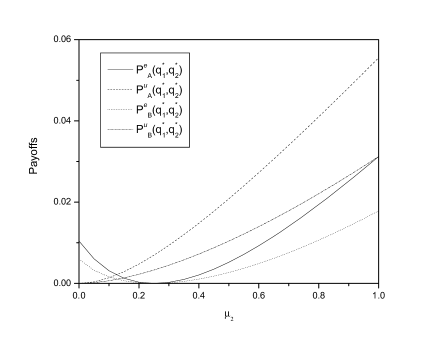
\put(-350.0,220.0){}

Figure 3: The payoffs ($P_{A}(q_{1}^{\ast},q_{2}^{\ast})$ and $P_{B}(q_{1}^{\ast},q_{2}^{\ast})$) are plotted at the subgame perfect Nash equilibrium point against the memory parameter $\mu_{2}$ both for entangled and unentangled initial states under the action of depolarizing channel, with the other parameters$\ p_{1}=\mu_{1}=0$, $k=1$ and $\ p_{2}=0.5$

The effect of quantum memory on firms’ payoffs for unentangled initial state under depolarizing channel is shown in figure $3$. The dashed line represents firm $A$’s payoff and dashed-dotted line represnets firm $B$’s payoff for unentangled initial state. The payoffs grow up with increasing value of memory parameter and the game remains the first mover advantage game.

When the initial state is maximally entangled and only the second decohering process is taken into account, the moves and payoffs of the firms for $k=1$ become

$$q_{1}^{\ast} = \frac{1}{2}+\frac{3}{4\{-3+2p_{2}(-3+2p_{2})(-1+\mu_{2})\}}$$

$$q_{2}^{\ast} = \frac{\{-3+2p_{2}(-3+2p_{2})(-1+\mu_{2})\}\{-3+4p_{2}(-3+2p_{2})(-1+\mu_{2})\}}{63+8p_{2}(-3+2p_{2})\{-9+2p_{2}(-3+2p_{2})(-1+\mu_{2})\}(-1+\mu_{2})}$$

$$P_{A} = -\frac{\{3-4p_{2}(-3+2p_{2})(-1+\mu_{2})\}^{2}}{96\{-3+2p_{2}(-3+2p_{2})(-1+\mu_{2})\}}$$

$$P_{B} = -\frac{\{3-4p_{2}(-3+2p_{2})(-1+\mu_{2})\}^{2}\{-3+2p_{2}(-3+2p_{2})(-1+\mu_{2})\}}{24[63+8p_{2}(-3+2p_{2})\{-9+2p_{2}(-3+2p_{2})(-1+\mu_{2})\}(-1+\mu_{2})]}$$

From equation (LABEL:23) one can easily check that no Nash equilibrium exists for decoherence parameter $p_{2}>0.32$ when the channel is uncorrelated. However, the presence of quantum correlations ensure the presence of Nash equilibrium for the entire range of decoherence parameter. It can be checked that for a given value of memory parameter the payoffs decrease when plotted as function of decoherence parameter and the game is always first mover advantage game. The dependence of payoffs for the maximally entangled initial state on the memory parameter is shown in figure $3$. The solid line in the figure represents firm $A$’s payoff and the dotted line represents firm $B$’s payoff for the maximally entangled initial state. It can be seen that the game is no-payoff game around $\mu_{2}=0.25$. For other values of memory parameter, the game is first mover advantage game and the firms are better off when the channel is fully correlated.

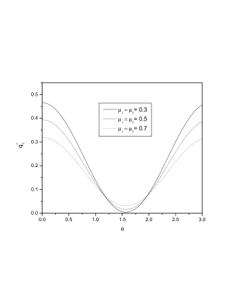
\put(-350.0,220.0){}

Figure 4: The payoffs ($P_{A}(q_{1}^{\ast},q_{2}^{\ast})$ and $P_{B}(q_{1}^{\ast},q_{2}^{\ast})$) are plotted at the subgame perfect Nash equilibrium point against the memory parameter $\mu_{2}$ both for entangled and unentangled initial states under the action of depolarizing channel, with the other parameters$\ p_{1}=\mu_{1}=0$, $k=1$ and $\ p_{2}=0.5$

To analyze the effect of entanglement in the initial state of the game on the Nash equilibrium, we plot the firms’ moves $q_{1}^{\ast}$, $q_{2}^{\ast}$ in figures $4$ and $5$, respectively. From figure 4, one can see that the move of the leader firm is positive for the whole range of entanglement angle. However, for memory parameters $\mu_{1}=\mu_{2}<0.5$, the move $q_{2}$ of the follower firm is negative for a particular range of values of entanglement parameter $\theta$ as can be seen from figure $5$.

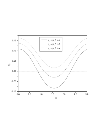
\put(-350.0,220.0){}

Figure 5: The move of firm $B$ at the subgame perfect Nash equilibrium point under the influence of depolarizing channel is plotted against the entanglement angle $\theta$ with other parameters$\ p_{1}=p_{2}=0.25$, $k=1$.

The negative value of $q_{2}$ shows that no Nash equilibrium of the game exists in this range of values of $\theta$. On the other hand, the existence of Nash equilibrium is ensured for the whole range of values of the entanglement parameter for highly correlated channel.

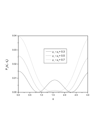
\put(-350.0,220.0){}

Figure 6: The payoff of firm $A$ at the subgame perfect Nash equilibrium point under the influence of depolarizing channel is plotted against the entanglement angle $\theta$ with other parameters$\ p_{1}=p_{2}=0.25$, $k=1$.

The payoffs of firms as function of entanglement parameter are plotted in figures $6$ and $7$. A local maximum exists at $\theta=\pi$ for smaller values of memory parameters which disappears for the values of memory parameters $>0.5$.

\put(-350.0,220.0){}

Figure 7: The payoff of firm $B$ at the subgame perfect Nash equilibrium point under the influence of depolarizing channel is plotted against the entanglement angle $\theta$ with the following values of the other parameters$\ p_{1}=p_{2}=0.25$, $k=1$.

4.3 Correlated phase damping channel

The diagonal elements of the final density matrix of the game when it evolves under the action of correlated phase damping channel are given by

$$\rho_{11}^{\prime} = q_{12}(\cos^{2}\theta+q_{1}q_{2}\sin^{2}\theta)$$

$$\rho_{22}^{\prime} = q_{12}(q_{2}\cos^{2}\theta+q_{1}\sin^{2}\theta)$$

$$\rho_{33}^{\prime} = q_{12}(q_{1}\cos^{2}\theta+q_{2}\sin^{2}\theta)$$

$$\rho_{44}^{\prime} = q_{12}(q_{1}q_{2}\cos^{2}\theta+\sin^{2}\theta)$$ (32)

The payoffs of firms in quantum Stackelberg duopoly game depend only on the diagonal elements of the final density matrix as can be seen from equations (11 and 12). It is clear from equation (32) that the diagonal elements of the final density matrix are independent of the decoherence parameters as well as from the memory parameters. Therefore, the correlated phase damping channel does not effect the outcome of the game.

5 Conclusions

We study the influence of entanglement and correlated noise on the quantum Stackelberg duopoly game by considering the time correlated amplitude damping, depolarizing and phase damping channels using Kraus operator formalism. We have shown that in different entangling regions the follower advantage can be enhanced or weakened due to the existence of the initial state entanglement influenced by different correlated noise channels. The problem of nonexistence of the subgame perfect Nash equilibrium in various regions due to the presence of decoherence is resolved by quantum memory.

It is shown that under the action of amplitude damping channel, for initially unentangled state, the presence of quantum memory results into a critical point at the subgame perfect Nash equilibrium. The firms are equally benefited at this point and the leader advantage vanishes. Beyond this critical point, the Nash equilibrium of the game gives higher payoff to the follower firm as a result of quantum memory, that is, the game converts from leader advantage to the follower advantage game. Quantum memory, in the case of amplitude damping channel, favors the follower firm in a particular range of values of entanglement parameter at the subgame perfect Nash equilibrium. In this range of values of entanglement parameter, the leader firm get worse off and the follower firm is better off (see figure 2). It is also observed that quantum memory validates the existence of Nash equilibrium for the whole range of entanglement angle and decoherence parameter. It is also shown that quantum memory in the case of phase damping channel has no effect on the subgame perfect Nash equilibrium and thus does not change the outcome of the game.

In the case of depolarizing channel quantum memory and entanglement in the initial state influences the firms’ payoffs at the subgame perfect Nash equilibrium strongly in a way different from amplitude damping channel. It is seen that for $p>0.32$, no Nash equilibrium exists in case of unentangled initial state. Whereas the presence of entanglement in the initial state extends the span of decoherence parameter $p$ from $0-0.32$ to $0-0.5$ for the existence of subgame perfect Nash equilibrium in the absence of quantum memory. On the other hand, we have observed that in the presence of memory, the subgame perfect Nash equilibrium exists for the entire range of decoherence parameter in both of the situations (for entangled and unentangled initial states). Similarly, it has been shown that memory has a striking effect that there exists a Nash equilibrium of the game for the entire range of entanglement parameter as well. Whereas, in the absence of memory, the noisy environment limits the subgame perfect Nash equilibrium to exist in a particular range of entanglement angle. In addition, a local maximum in payoffs is observed for small values of quantum memory parameters $\mu_{1}$, $\mu_{2}$. For highly correlated channel this local maximum disappears and the payoffs reduce to zero. Unlike amplitude damping channel, the correlated depolarizing channel does not give rise to a critical point at the subgame perfect Nash equilibrium and as a result, the game always remains a leader advantage game.

6 Acknowledgment

We would like to thank the referees of Journal of Physics A: Mathematical and Theoretical, for their substantial contribution to the improvement of the manuscript by their useful suggestions. One of the authors (Salman Khan) is thankful to World Federation of Scientists for partially supporting this work under the National Scholarship Program for Pakistan.

Appendix A

The damping functions $A_{i}$ in equation (15) are given as

$$A_{1} = \frac{1}{2}[-k-4(-1+p_{1})(-1+p_{2})p_{2}(-1+\mu_{2})$$ (33)

$$-2kp_{2}(p_{2}+\mu_{2}-p_{2}\mu_{2})-2kp_{1}[\mu_{1}+p_{2}\{2-p_{2}(-2+\mu_{1})$$

$$\times(-1+\mu_{2})-4\mu_{2}+\mu_{1}(-2+3\mu_{2})\}]$$

$$-k\cos 2\theta+4(-1+p_{1})(-1+p_{2})p_{2}(-1+\mu_{2})\cos 2\theta$$

$$+2kp_{2}(p_{2}+\mu_{2}-p_{2}\mu_{2})\cos 2\theta+2kp_{1}[\mu_{1}+p_{2}\{2-p_{2}(-2+\mu_{1})$$

$$\times(-1+\mu_{2})-4\mu_{2}+\mu_{1}(-2+3\mu_{2})\}]\cos 2\theta]-2p_{1}(-1+\mu_{1})$$

$$\times[2+p_{1}[-2+k\{-1+p_{2}(2-3\mu_{2})+p_{2}^{2}(-1+\mu_{2})\}$$

$$-4p_{2}(-1+\mu_{2})+2p_{2}^{2}(-1+\mu_{2})]+4p_{2}(-1+\mu_{2})$$

$$-2p_{2}^{2}(-1+\mu_{2})]\sin^{2}\theta$$

$$A_{2} = -4(1+k)p_{2}(-1+\mu_{2})-4(-1+p_{1})p_{1}(-1+\mu_{1})$$ (34)

$$\times[-2+k\{-1+p_{2}(2-3\mu_{2})+p_{2}^{2}(-1+\mu_{2})\}$$

$$-4p_{2}(-1+\mu_{2})+2p_{2}^{2}(-1+\mu_{2})]\sin^{2}\theta$$

The damping functions $B_{i}$ in equation (15) are given as

$$B_{1} = -2+\frac{1}{8}k[1+2p_{2}(p_{2}+\mu_{2}-p_{2}\mu_{2})$$

$$+2p_{1}[\mu_{1}+p_{2}\{2-4\mu_{2}+\mu_{1}(-2+3\mu_{2})\}]$$

$$+[1-2[p_{2}(p_{2}+\mu_{2}-p_{2}\mu_{2})+p_{1}\{\mu_{1}+p_{2}(2-2\mu_{1}$$

$$-4\mu_{2}+3\mu_{1}\mu_{2})\}]]\cos 2\theta]-\frac{1}{2}p_{1}(-1+\mu_{1})[k(-4+3p_{1})$$

$$\times\{-1+p_{2}(2-3\mu_{2})+p_{2}^{2}(-1+\mu_{2})\}+6(-1+p_{1})\{-1-2p_{2}$$

$$\times(-1+\mu_{2})+p_{2}^{2}(-1+\mu_{2})\}]\sin^{2}\theta-\frac{1}{2}p_{2}(-1+\mu_{2})$$

$$\times[4(1+k)+[2(-1+p_{2})+p_{1}\{2+p_{2}(-2+k(-2+\mu_{1}))\}]\sin^{2}\theta]$$

$$B_{2} = -16+2[2\{-1-(1+k)p_{2}(-1+\mu_{2})\}+p_{1}^{2}(-1+\mu_{1})$$ (36)

$$\times[(2+k)(-1+p_{2})^{2}+p_{2}\{4+3k-(2+k)p_{2}\}\mu_{2}]$$

$$+p_{1}(-1+\mu_{1})[-(2+k)(-1+p_{2})^{2}+p_{2}\{-4-3k$$

$$+(2+k)p_{2}\}\mu_{2}]+(-1+p_{1})p_{1}(-1+\mu_{1})[-(2+k)(-1+p_{2})^{2}$$

$$+p_{2}\{-4-3k+(2+k)p_{2}\}\mu_{2}]\cos 2\theta][\{1+(1+k)p_{2}$$

$$\times(-1+\mu_{2})\}\cos^{2}\theta+[1+(1+k)p_{2}(-1+\mu_{2})+p_{1}(-1+\mu_{1})$$

$$\times[(2+k)(-1+p_{2})^{2}+p_{2}\{4+3k-(2+k)p_{2}\}\mu_{2}]$$

$$+p_{1}^{2}(-1+\mu_{1})[-(2+k)(-1+p_{2})^{2}+p_{2}\{-4-3k$$

$$+(2+k)p_{2}\}\mu_{2}]\sin^{2}\theta]-[-2(-1+p_{1})[p_{1}(-1+\mu_{1})$$

$$\times\{-1+(-2+p_{2})p_{2}(-1+\mu_{2})\}+(-1+p_{2})p_{2}(-1+\mu_{2})]$$

$$-k[1+p_{2}(p_{2}+\mu_{2}-p_{2}\mu_{2})+p_{1}^{2}(-1+\mu_{1})\{-(-1+p_{2})^{2}$$

$$+(-3+p_{2})p_{2}\mu_{2}\}+p_{1}[\mu_{1}+p_{2}\{2-p_{2}(-2+\mu_{1})(-1+\mu_{2})$$

$$-4\mu_{2}+\mu_{1}(-2+3\mu_{2})\}]]+(-1+p_{1})[2\{p_{1}(-1+\mu_{1})$$

$$\times\{-1+(-2+p_{2})p_{2}(-1+\mu_{2})\}+(-1+p_{2})p_{2}(-1+\mu_{2})\}$$

$$+k[(-1+p_{2})\{-1+p_{2}(-1+\mu_{2})\}+p_{1}(-1+\mu_{1})\{-(-1+p_{2})^{2}$$

$$+(-3+p_{2})p_{2}\mu_{2}\}]]\cos 2\theta][p_{2}\{-2-(2+k)p_{2}(-1+\mu_{2})$$

$$+(2+k)\mu_{2}\}\cos^{2}\theta+[2p_{1}[-1+\mu_{1}+p_{1}(-1+\mu_{1})$$

$$\times\{-1+(-2+p_{2})p_{2}(-1+\mu_{2})\}-p_{2}\{1+(-2+p_{2})\mu_{1}\}(-1+\mu_{2})]$$

$$+k[1+p_{1}[-2+\mu_{1}+p_{1}(-1+\mu_{1})\{-(-1+p_{2})^{2}+(-3+p_{2})p_{2}\mu_{2}\}$$

$$+p_{2}\{2-2\mu_{2}+\mu_{1}(-2+p_{2}+3\mu_{2}-p_{2}\mu_{2})\}]]]\sin^{2}\theta]$$

The damping functions $A_{i}^{\prime}$ in equation (28) are given as

$$A_{1}^{\prime} = 4(2+k)p_{1}(-3+2p_{1})(-1+\mu_{1})\{-9+8p_{2}(-3+2p_{2})$$ (37)

$$\times(-1+\mu_{2})\}-36(2+k)p_{2}(-3+2p_{2})(-1+\mu_{2})$$

$$+\frac{9}{2}k[9+\{9-24p_{2}+8p_{1}(-3+4p_{2})\}\cos 2\theta]$$

$$A_{2}^{\prime} = 8(2+k)[p_{1}(-3+2p_{1})(-1+\mu_{1})\{-9+8p_{2}(-3+2p_{2})$$ (38)

$$\times(-1+\mu_{2})\}-9p_{2}(-3+2p_{2})(-1+\mu_{2})]$$

The damping functions $B_{i}^{\prime}$ in equation (28) are given as

$$B_{1}^{\prime} = 8(2+k)^{2}(3-2p_{2})^{2}p_{2}^{2}\{9-8p_{1}(-3+2p_{1})(-1+\mu_{1})\}^{2}$$ (39)

$$\times[k\{-9+4p_{1}(-3+2p_{1})(-1+\mu_{1})\}+8p_{1}(-3+2p_{1})$$

$$\times(-1+\mu_{1})-k(-3+4p_{1})(-3+4p_{2})\cos 2\theta]+18(2+k)$$

$$\times p_{2}(-3+2p_{2})\{-9+8p_{1}(-3+2p_{1})(-1+\mu_{1})\}(-1+\mu_{2})$$

$$\times[(2+k)\{9-8p_{1}(-3+2p_{1})(-1+\mu_{1})\}+k(-3+4p_{1})$$

$$\times(-3+4p_{2})\cos 2\theta]$$

$$B_{2}^{\prime} = -72(2+k)p_{2}(-3+2p_{2})[4\{-9+2p_{1}(-3+2p_{1})(-1+\mu_{1})\}$$ (40)

$$+k\{9+4p_{1}(-3+2p_{1})(-1+\mu_{1})\}]\{-9+8p_{1}$$

$$\times(-3+2p_{1})(-1+\mu_{1})\}(-1+\mu_{2})+16(2+k)^{2}(3-2p_{2})^{2}$$

$$\times p_{2}^{2}\{9-8p_{1}(-3+2p_{1})(-1+\mu_{1})\}^{2}(-1+\mu_{2})^{2}$$

$$+81[k^{2}\{-81+8p_{1}(-3+2p_{1})\{9+2p_{1}(-3+2p_{1})(-1+\mu_{1})\}$$

$$\times(-1+\mu_{1})\}+64p_{1}(-3+2p_{1})\{-9+p_{1}(-3+2p_{1})$$

$$\times(-1+\mu_{1})\}(-1+\mu_{1})+16kp_{1}(-3+2p_{1})\{-9+4p_{1}$$

$$\times(-3+2p_{1})(-1+\mu_{1})\}(-1+\mu_{1})+k^{2}(3-4p_{1})^{2}$$

$$\times(3-4p_{2})^{2}\cos^{2}2\theta]$$

References

• [1] von Neumann J 1951 Appl. Math. Ser. 12 36
• [2] Piotrowski E W, Sladkowski J 2002 Physica A 312 208
• [3] Baaquie B E 2001 Phys. Rev. E 64
• [4] Nielson M A ,Chuang I L 2000 Quantum Computation and Quantum Information ( Cambridge: Cambridge University Press)
• [5] Eisert J, Wilkens M and Lewenstein M 1999 Phy. Rev. Lett 83 3077
• [6] Benjamin S C and Hayden P M 2001 Phys. Rev. Lett. 87 0689801
• [7] Marinatto L and Weber T 2001 Phys. lett. A 280 249
• [8] Li CΒ F et al. 2001 Phys. Lett. A 280 257
• [9] Lo CΒ F, Kiang D 2003 Phys Lett. A 318 333
• [10] Flitney AΒ P and Abbott D 1999 Phys. Rev. A 65 062318
• [11] P. Gawron et al 2008 IJTP 6 667
• [12] I. Pakula 2008 Fluctuation and Noise Letters 8 L23
• [13] Meyer DΒ A 1999 Phys. Rev. Lett. 82 1052
• [14] Piotrowski E and Sladowski J 2004 The next stage: quantum game theory, in CV Benton (ed.), Mathematical Physics Research at Cutting Edge, Hauppauge, NY, p. 251
• [15] Iqbal A 2004 Studies in the Theory of Quantum Games, Ph.D thesis, Quaid-i-Azam University, Department of Electronics
• [16] Cheon T and Tsutsui I 2006 Phys. Lett. A 348 147
• [17] Ichikawa T and Tsutsui I 2007 Ann. Phys. 322 531
• [18] Iqbal A and Cheon T 2007 Phys. Rev. Lett. E 76 061122
• [19] Ichikawa T, Tsutsui I and Cheon T 2008 J. Phys. A: Math. Theor. 41 135303
• [20] Zhu X and Kuang LΒ M 2007 J. Phys. A: Math. Theor. 40 7729
• [21] Zhu X and Kuang LΒ M 2008 Commun. Theor. Phys. 49 111
• [22] Zurek W H et al. 1991 Phys. Today 44 36
• [23] Macchiavello C and Palma G M 2002 Phys. Rev. A 65 050301R
• [24] Yeo Y and Skeen A 2003 Phys. Rev. A 67 064301
• [25] Chen LΒ K, Ang H, Kiang D, Kwek LΒ C and Lo CΒ F 2003 Phys. Lett. A 316 317
• [26] Flitney AΒ PΒ and Hollenberg LΒ CΒ L 2007 Quant. Inform. Comput. 7 111
• [27] Khan S, Ramzan M and Khan M K 2010 Int. J. Theor. Phys. 49 31
• [28] Ramzan M et al. 2008 J. Phys. A: Math. Theor. 40 055307
• [29] Ramzan M and Khan MΒ K 2008 J. Phys. A: Math. Theor.Β 40 435302
• [30] Gibbons R 1992 Game theory for Applied Economists (Princeton University Press, Princeton, NJ)
• [31] Li H, Du J and Massar S 2002 Phys. Lett. A 306 73
• [32] Marinatto L and Weber T 2000 Phys. Lett. A 272 291
• [33] Iqbal A and Toor A H 2002 Phys. Rev. AΒ 65 052328
• [34] Lo F and Kiang 2005 Phys Lett A 346 65