Abstract

One of the main challenges of the Tevatron at Fermilab and the Large Hadron Collider (LHC) at CERN is the determination of Standard Model (SM) parameters at the TeV scale. In this context various processes will be investigated which involve bottom-quark jets in the final state, for example decays of top-quarks or gauge bosons of the weak interaction. Hence the theoretical understanding of processes with bottom-quark jets is necessary. In this paper analytic results will be presented for the weak corrections to bottom-quark jet production — neglecting purely photonic corrections. The results will be used to study differential distributions, where sizeable effects are observed.

I Introduction

With the start of the LHC a new energy regime is accessible, either to confirm the Standard Model (SM) or to verify new physics at the TeV scale. Famous possible SM extensions are heavy gauge bosons (e.g. $Z^{\prime}$), Supersymmetry or Kaluza-Klein resonances in models with extra dimensions. Beside the outstanding discovery of the Higgs boson, processes involving top-quarks, gauge bosons of the weak interaction and jets are of particular interest. The experimental identification will rely on their characteristic decay products with leptons or bottom jets as characteristic examples. In particular in processes including top-quarks or a (light) Higgs boson the identification of the bottom-quark jets will play a crucial role. In addition to these SM processes, bottom-quark jets are also involved in many decays originating from signals for physics beyond the SM. In particular new resonances, e.g. heavy gauge bosons, decaying into $b$-jets require a detailed SM-based prediction to prove a deviation from the SM. The discrimination of $b$-jets from light quark- and gluon-jets, $b$-tagging, makes use of the large lifetime of B-mesons. In the last years there were large efforts by several experimental groups to develop new or to improve established $b$-tagging algorithms. This requires a detailed theoretical understanding of the corresponding processes like bottom-quark pair and single bottom-quark production. Both processes were studied in the past. The differential cross section for bottom-quark pair production is known to next-to-leading order (NLO) accuracy in quantum chromodynamics (QCD) [1, 2]. For massless single bottom production the NLO QCD corrections can be extracted from di-jet production [3, 4].

It is well known that weak corrections can also be significant because of the presence of possible large Sudakov logarithms. These effects were studied intensively for several processes like weak boson, jet and top-quark pair production [5, 6, 7, 8, 9, 10, 11, 12, 13]. Earlier work on Sudakov logarithms in four-fermion processes can be found in Refs. [14, 15, 16, 17, 18, 19, 20, 21, 23]. A first study for $b\bar{b}$ production can be found in Ref. [24], where the partonic sub-processes $gg\rightarrow b\bar{b}$ and $q\bar{q}\rightarrow b\bar{b}$ were considered.

In experimental studies, e.g. of top-quark pair production at the Tevatron, often only one $b$-jet is required. Considering the importance of these background studies also single bottom-quark production will be studied in this paper.

The outline of the paper is as follows: In Section II the leading-order cross sections for the production of one and two bottom jets are presented. The partonic contributions are split into quark-, gluon- and pure bottom-induced processes and relations based on crossing symmetries are introduced. After a discussion at the hadronic level we find, that leading order processes involving electroweak gauge boson exchange can be neglected. Concerning the differential ${p_{\rm T}}$ distribution at high energies the effects from pure bottom-induced contributions are also negligible. In Section III we present the virtual and real corrections of order $\alpha_{s}^{2}\alpha$ for the remaining processes. The virtual contributions to quark-induced processes contain infrared and ultraviolet singularities, while the gluon-induced ones are infrared finite. Compact analytic expressions for the various channels are presented. In Section IV we present various consistency tests of our calculation and discuss the numerical results at the hadronic level. Our conclusions are given in Section V.

II Bottom-jet production at leading-order

At parton level three types of processes will be distinguished: Quark-induced processes (with two quarks in the initial state, one of these being $u,d,c,s$), gluon-induced contributions (with one or two gluons in the initial state) and finally pure bottom-quark induced processes:

$${\rm quark-induced}: q\bar{q}\rightarrow b\bar{b},\>\>\bar{b}q\rightarrow\bar{b}q,\>\>b\bar{q}\rightarrow b\bar{q},\>\>bq\rightarrow bq,\>\>\bar{b}\bar{q}\rightarrow\bar{b}\bar{q},$$ (II.1)

$${\rm gluon-induced}: gg\rightarrow b\bar{b},\>\>bg\rightarrow bg,\>\>\bar{b}g\rightarrow\bar{b}g,$$

$${\rm bottom-induced}: b\bar{b}\rightarrow b\bar{b},\>\>bb\rightarrow bb,\>\>\bar{b}\bar{b}\rightarrow\bar{b}\bar{b}.$$

Processes with initial state photons are neglected. Here the light quarks (denoted generically by $q$ and $\bar{q}$) and the bottom-quark ($b$ and $\bar{b}$) are taken as massless. Sample diagrams are shown in Fig. II.2 and Fig. II.2. The colour and spin averaged squared matrix element $\overline{\sum}|{{\cal M}}^{i,j\rightarrow k,l}|^{2}$ can be written either in terms of the Mandelstam variables $s$, $t$ and $u$ or as a function of $s$ and the cosine of the scattering angle $\cos\vartheta=z=(u-t)/s$

$$\overline{\sum}|{{\cal M}}^{i,j\rightarrow k,l}|^{2}(s,t,u)=\overline{\sum}|{{\cal M}}^{i,j\rightarrow k,l}|^{2}(s,z).$$ (II.2)

Various explicitly checked crossing relations will be useful below. For the quark-induced processes in Eq. (II.1) we find

$$\overline{\sum}|{{\cal M}}^{q\bar{b}\rightarrow q\bar{b}}|^{2}=\overline{\sum}|{{\cal M}}^{\bar{q}b\rightarrow\bar{q}b}|^{2} = \overline{\sum}|{{\cal M}}^{q\bar{q}\rightarrow b\bar{b}}|^{2}\Big{|}_{s\leftrightarrow t},$$

$$\overline{\sum}|{{\cal M}}^{qb\rightarrow qb}|^{2}=\overline{\sum}|{{\cal M}}^{\bar{q}\bar{b}\rightarrow\bar{q}\bar{b}}|^{2} = \overline{\sum}|{{\cal M}}^{\bar{q}b\rightarrow\bar{q}b}|^{2}\Big{|}_{s\leftrightarrow u}$$ (II.3)

$$= \overline{\sum}|{{\cal M}}^{q\bar{q}\rightarrow b\bar{b}}|^{2}\Big{|}_{s\rightarrow t,\>\>t\rightarrow-s,\>\>u\rightarrow-u}$$

and similarly for gluon-induced and pure bottom-induced processes

$$\overline{\sum}|{{\cal M}}^{gb\rightarrow gb}|^{2}=\overline{\sum}|{{\cal M}}^{g\bar{b}\rightarrow g\bar{b}}|^{2}=-\overline{\sum}|{{\cal M}}^{gg\rightarrow b\bar{b}}|^{2}\Big{|}_{s\leftrightarrow t},$$ (II.4)

$$\overline{\sum}|{{\cal M}}^{bb\rightarrow bb}|^{2}=\overline{\sum}|{{\cal M}}^{\bar{b}\bar{b}\rightarrow\bar{b}\bar{b}}|^{2}=\overline{\sum}|{{\cal M}}^{b\bar{b}\rightarrow b\bar{b}}|^{2}\Big{|}_{s\leftrightarrow u}.$$ (II.5)

The spin and colour averaged differential partonic cross section reads

$${{\rm d}\sigma^{i,j\rightarrow k,l}\over{\rm d}z}={1\over I}{1\over 32\pi s}\overline{\sum}|{{\cal M}}^{i,j\rightarrow k,l}|^{2}(s,z)$$ (II.6)

where $I=2$ for identical particles in the final state and $I=1$ otherwise.
Before presenting explicit results we complete the notation and definitions used in this and the following Sections. As usual $\alpha_{s}$ and $\alpha$ stand for the strong and electromagnetic coupling constant. The $Z$ boson mass is denoted by ${m_{Z}}$ and the (axial-)vector coupling is expressed in terms of the sine (cosine) of the weak mixing-angle ${s_{W}}$ (${c_{W}}$), the weak isospin $T_{3}^{f}$ and the electric charge $Q_{f}$ for a fermion of flavour $f$ in units of the elementary charge $e$:

$$g_{v}^{f} = {1\over 2{s_{W}}{c_{W}}}(T_{3}^{f}-2{s_{W}}^{2}Q_{f}),\quad g_{a}^{f}={1\over 2{s_{W}}{c_{W}}}T_{3}^{f}.$$ (II.7)

The Cabibbo-Kobayashi-Maskawa mixing matrix is set to 1 and the $W$ coupling to the quarks is

$${g_{W}}={1\over 2\sqrt{2}{s_{W}}}.$$ (II.8)

Let us start with the processes listed in Eq. (II.1), which involve only quarks in the initial state. These can be mediated by gluon, $Z$ boson and photon exchange. Consequently we seperate pure QCD ${\rm O}(\alpha_{s}^{2})$, electroweak ${\rm O}(\alpha^{2})$, and mixed QCD-electroweak ${\rm O}(\alpha_{s}\alpha)$ contributions. In the case of one or two gluons in the initial-state an interaction via electroweak gauge bosons is not possible at leading order and only QCD processes contribute. We start with the QCD-contribution for quark–antiquark annihilation into a $b\bar{b}$-pair

$$\overline{\sum}|{{\cal M}}_{\alpha_{s}^{2}}^{q\bar{q}\rightarrow b\bar{b}}|^{2}\Big{(}s,z(s,t,u)\Big{)}=4\*\alpha_{s}^{2}\*\pi^{2}{N^{2}-1\over N^{2}}\*(1+z^{2}),$$ (II.9)

with $N$ being the number of colors. The purely electroweak contributions are given by

$$\overline{\sum}|{{\cal M}}_{\alpha^{2}}^{q\bar{q}\rightarrow b\bar{b}}|^{2}\Big{(}s,z(s,t,u)\Big{)}=16\*\alpha^{2}\*\pi^{2}\*\Big{[}Q_{b}^{2}\*Q_{q}^{2}\*(1+z^{2})$$

$$\quad\quad+\quad{s^{2}\over(s-{m_{Z}}^{2})^{2}}\*\Big{(}({g_{v}^{q}}^{2}+{g_{a}^{q}}^{2})\*({g_{v}^{b}}^{2}+{g_{a}^{b}}^{2})\*(1+z^{2})-8\*{g_{v}^{q}}\*{g_{v}^{b}}\*{g_{a}^{q}}\*{g_{a}^{b}}\*z\Big{)}$$

$$\quad\quad+\quad 2\*{s\over s-{m_{Z}}^{2}}\*Q_{q}\*Q_{b}\*\Big{(}{g_{v}^{q}}\*{g_{v}^{b}}\*(1+z^{2})-2\*{g_{a}^{q}}{g_{a}^{b}}\*z\Big{)}\Big{]}.$$ (II.10)

Because of colour conservation the interference between the QCD and electroweak matrix elements vanish. The remaining quark-induced contributions can be obtained using the crossing relations in Eq. (II.3).
The gluon-induced processes in Eq. (II.1) proceed through QCD amplitudes only and the corresponding crossing relations are defined in Eq. (II.4). For the gluon fusion channel the squared matrix element is

$$\overline{\sum}|{{\cal M}}_{\alpha_{s}^{2}}^{gg\rightarrow b\bar{b}}|^{2}\Big{(}s,z(s,t,u)\Big{)}=8\alpha_{s}^{2}\*\pi^{2}\*{1\over N(N^{2}-1)}\*(N^{2}-2+N^{2}z^{2}){1+z^{2}\over 1-z^{2}}.$$ (II.11)

Finally we consider the pure bottom-quark induced contributions arising from pure QCD, mixed QCD-electroweak and electroweak matrix elements. Below we list the results for $b\bar{b}\rightarrow b\bar{b}$ scattering, those for $bb\rightarrow bb$ and $\bar{b}\bar{b}\rightarrow\bar{b}\bar{b}$ scattering can be deduced from Eq. (II.5).

$$\overline{\sum}|{{\cal M}}_{\alpha_{s}^{2}}^{b\bar{b}\rightarrow b\bar{b}}|^{2}\Big{(}s,z(s,t,u)\Big{)} = 4\*\alpha_{s}^{2}\*\pi^{2}\*{N^{2}-1\over N^{3}}$$

$$\times {2\*(1-z)\*(1-z^{2})+N\*(11-2\*z+4\*z^{2}+2\*z^{3}+z^{4})\over(1+z)^{2}},$$

$$\overline{\sum}|{{\cal M}}_{\alpha_{s}\alpha}^{b\bar{b}\rightarrow b\bar{b}}|^{2}\Big{(}s,z(s,t,u)\Big{)} = -16\*\alpha\*\alpha_{s}\*\pi^{2}\*{N^{2}-1\over N^{2}}\*\Big{[}2\*Q_{b}^{2}\*{(1-z)^{2}\over 1+z}$$

$$+ ({g_{v}^{b}}^{2}+{g_{a}^{b}}^{2})\*{s\over s-{m_{Z}}^{2}}\*{(1-z)^{2}\over 1+z}\*{2\*s\*(1+z)+{m_{Z}}^{2}\*(1-z)\over s\*(1+z)+2\*{m_{Z}}^{2}}\Big{]},$$

$$\overline{\sum}|{{\cal M}}_{\alpha^{2}}^{b\bar{b}\rightarrow b\bar{b}}|^{2}\Big{(}s,z(s,t,u)\Big{)} = 16\*\alpha^{2}\*\pi^{2}$$ (II.14)

$$\times \Bigg{[}Q_{b}^{4}\*{N\*(11-2\*z+4\*z^{2}+2\*z^{3}+z^{4})-2\*(1-z)\*(1-z^{2})\over N\*(1+z)^{2}}$$

$$+ {s^{2}\over N\*(s-{m_{Z}}^{2})^{2}\*(s\*(1+z)+2\*{m_{Z}}^{2})^{2}}$$

$$\times \Big{[}({g_{v}^{b}}^{4}+{g_{a}^{b}}^{4})\*\Big{(}2\*{m_{Z}}^{4}\*(2\*(1-z)^{2}+N\*(7-2\*z+3\*z^{2}))$$

$$- 2\*s\*{m_{Z}}^{2}\*(1-z)\*((1-z)^{2}+2\*N\*(4+z+z^{2}))$$

$$- s^{2}\*(2\*(1+z)\*(1-z)^{2}-N\*(11-2\*z+4\*z^{2}+2\*z^{3}+z^{4}))\Big{)}$$

$$+ {g_{a}^{b}}^{2}\*{g_{v}^{b}}^{2}\*\Big{(}4\*{m_{Z}}^{4}\*(6\*(1-z)^{2}+N\*(1-14\*z+5\*z^{2}))$$

$$- 4\*s\*{m_{Z}}^{2}\*(1-z)\*(3\*(1-z)^{2}-2\*N\*(2+5\*z-z^{2}))$$

$$- 2\*s^{2}\*(6\*(1+z)\*(1-z)^{2}+N\*(1+14\*z+2\*z^{3}-z^{4}))\Big{)}\Big{]}$$

$$- 2\*Q_{b}^{2}\*{s\over N\*(1+z)\*(s-{m_{Z}}^{2})\*(s\*(1+z)+2{m_{Z}}^{2})}$$

$$\times \Big{[}{g_{v}^{b}}^{2}\*\Big{(}{m_{Z}}^{2}\*\*(1-z)\*((1-z)^{2}+2\*N\*(4+z+z^{2}))$$

$$+ s\*(2\*(1+z)\*(1-z)^{2}-N\*(11-2\*z+4\*z^{2}+2\*z^{3}+z^{4}))\Big{)}$$

$$+ {g_{a}^{b}}^{2}\*\Big{(}{m_{Z}}^{2}\*(1-z)\*((1-z)^{2}-6\*N\*(1+z))$$

$$+ 2\*s\*(1+z)\*((1-z)^{2}+N\*(3+z^{2}))\Big{)}\Big{]}\Bigg{]}.$$

The term proportional to $\alpha{\alpha_{s}}$ originates from the interference between $s$ and $t$ exchange amplitudes and is present for the process $b\bar{b}\rightarrow b\bar{b}$ and its crossed versions only. The purely electroweak contributions proportional $\alpha^{2}$ are found to be negligible.

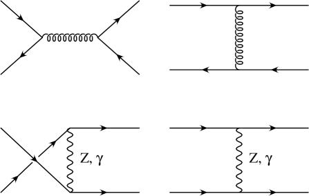
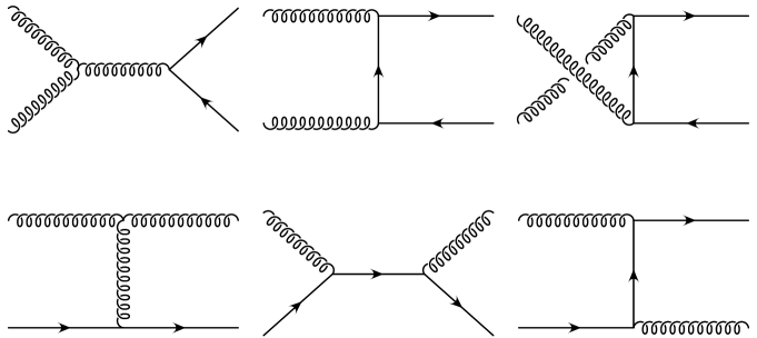
Figure II.1: Sample Born diagrams for quark-induced bottom-quark production.

Figure II.2: Sample Born diagrams for gluon-induced bottom-quark production.

With these ingredients we calculate the hadronic transverse momentum (${p_{\rm T}}$) distributions for single and double $b$-tag events and investigate the relative importance of the different processes described above. As a consequence of the massless approximation, most partonic contributions are ill-defined in the limit $z\to\pm 1$, where initial and final state parton become collinear. Since $b$-jets close to the beam pipe escape detection, we require a minimal transverse momentum ($p_{\rm T}^{\rm cut}$) of 50 GeV. The leading order cross section is obtained from

$${\rm d}\sigma_{H_{1},H_{2}\rightarrow X} = \sum_{i,j}\int_{0}^{1}{\rm d}x_{1}\int_{0}^{1}{\rm d}x_{2}f_{i/H_{1}}(x_{1})f_{j/H_{2}}(x_{2})$$ (II.15)

$$\times {\rm d}\hat{\sigma}_{i,j\rightarrow X}(x_{1}P_{1},x_{2}P_{2})\>\>\>\Theta({p_{\rm T}}>p_{\rm T}^{\rm cut}),$$

where the factorization scale dependence is suppressed and $x_{1}$ and $x_{2}$ are the partonic momentum fractions. The parton distribution functions (PDF’s) for parton $i$ in hadron $H$ are denoted by $f_{i/H}$. The sum runs over all possible parton configurations $(i,j)$ in the initial state.

For the study of $b$-jets we will distinguish between single $b$-tag and double $b$-tag events, and evaluate the ${p_{\rm T}}$ distributions with the following input parameters

$$\alpha_{s}=0.1,\quad\alpha={1\over 128},\quad{m_{Z}}=91.1876~{}{\rm GeV},\quad{m_{W}}=80.425~{}{\rm GeV}.$$ (II.16)

For ${s_{W}}$ we use the on-shell relation. Moreover we used the PDF’s from CTEQ6L with the factorisation scale set to ${\mu_{F}}=2p_{\rm T}^{\rm cut}$.

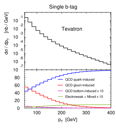
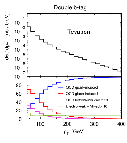
Figure II.3: Differential cross section as a function of ${p_{\rm T}}$ for single $b$-tag events (upper left figure) and double $b$-tag events (upper right figure) at the Tevatron ($\sqrt{s}=1.96$ TeV) and the relative composition normalized to the Born cross section (lower figures)

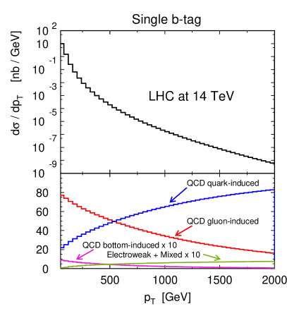
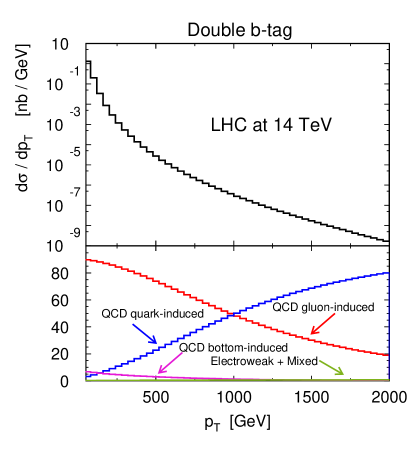
Figure II.4: Differential cross section as a function of ${p_{\rm T}}$ for single $b$-tag events (upper left figure), double $b$-tag events (upper right figure) at the LHC ($\sqrt{s}=14$ TeV) and the relative composition normalized to the Born cross section (lower figures)

Let us first discuss the results for the Tevatron ($\sqrt{s}=$ 1.96 TeV). The composition of the corresponding leading-order differential cross section for single $b$-tag events is shown in Fig. II.3(a). In the upper plot the cross section is depicted as a function of the transverse momentum ${p_{\rm T}}$, its relative composition in percent is shown below. For ${p_{\rm T}}$-values up to 200 GeV the gluon- and quark-induced QCD processes are of the same order, while for higher energies the quark-induced $b$-jet production is dominating the ${p_{\rm T}}$-distribution. Contributions from gluon-induced processes drop fast with increasing ${p_{\rm T}}$ and contribute only a few percent to the differential cross section for ${p_{\rm T}}>300$ GeV. The relative contributions from bottom-induced processes and processes with electroweak boson exchange are only of the order of few permille and therefore negligible for the ${p_{\rm T}}$-values considered.
For ${p_{\rm T}}<100$ GeV and in the double $b$-tag case the ${p_{\rm T}}$-distribution (Fig. II.3(b)) is dominated by the gluon fusion channel. For higher ${p_{\rm T}}$-values QCD quark–antiquark annihilation takes over and for transverse momenta larger than 200 GeV it dominates completely. The relative contributions from processes involving electroweak bosons are of the order of $1\%$ for ${p_{\rm T}}<80$ GeV and, for ${p_{\rm T}}>260$ GeV are of the same order (few permille) as the gluon-fusion process. Bottom-induced contributions yield a few percent to the differential cross section for ${p_{\rm T}}<100$ GeV and become insignificant for higher transverse momenta.
For the LHC the results are significantly different. The LO ${p_{\rm T}}$-distribution for single $b$-tag events is presented in Fig. II.4(a). The gluon-induced processes dominate in the low energy regime (${p_{\rm T}}<500$ GeV). For ${p_{\rm T}}$ larger than 500 GeV the quark-induced processes take over and finally dominate the distribution. This "cross over" of gluon- and quark-induced contributions is a consequence of the different behaviour of LHC quark and gluon luminosities. The relative contributions from the exchange of electroweak bosons and bottom-induced processes are always below $1\%$ and therefore negligible. A similiar picture is observed for the differential cross section for double $b$-tag events at the LHC (Fig. II.4(b)). Here the "cross over" of quark- and gluon-induced contributions is around ${p_{\rm T}}=1$ TeV. For low ${p_{\rm T}}$ the pure bottom-induced processes are as important as quark-induced contributions. This seems surprising, because the parton luminosities of bottom-quarks in a proton should be highly suppressed compared to the light flavours. There are two reasons for the relatively large cross section of the purely bottom-induced processes. First, the partonic cross sections of $bb$ and $b\bar{b}$ scattering are strongly enhanced for large $z$ values. In this region the parton processes with bottom-quarks in the initial state can be several orders of magnitude larger than the quark–antiquark-induced process. Second, the bottom-quark PDF is essentially obtained by multiplying the gluon distribution in the proton with the splitting function of a gluon into a bottom-quark pair. Because of the high gluon luminosities at low energies, the bottom-quark PDF becomes of the order of a few percent relative to the PDF’s of the light flavours. This, together with the large partonic contributions is responsible for the relatively large bottom-induced differential cross section. The argumentation implies that the main contribution from $bb$, $\bar{b}\bar{b}$ and $b\bar{b}$ scattering comes from the low ${p_{\rm T}}$ region, while for high ${p_{\rm T}}$ values these effects are small. It might be interesting to study whether the $b$-PDF could be further constrained using $b\bar{b}$ production at low ${p_{\rm T}}$.

As shown above, the leading order contributions from electroweak gauge boson exchange are always negligible for the study of $b$-jet production. This is also true in the context of NLO corrections with an expected size of serveral percent relative to the leading order distributions. Moreover, we have shown that the QCD contributions from processes with two bottom-quarks in the initial state are unimportant for the study of ${p_{\rm T}}$-distributions at large transverse momentum. In particular with regard to the Sudakov logarithms becoming important at high energies this approximation is justified. Consequently the weak ${\rm O}(\alpha)$ corrections to $bb\rightarrow bb$, $\bar{b}\bar{b}\rightarrow\bar{b}\bar{b}$ and $b\bar{b}\rightarrow b\bar{b}$ will not be discussed in this article.

III Weak corrections to bottom-quark production

In this Section we calculate the weak corrections of order $\alpha_{s}^{2}\alpha$ to the following partonic processes

$$\>\>q\bar{q}\rightarrow b\bar{b},\>\>\bar{b}q\rightarrow\bar{b}q,\>\>b\bar{q}\rightarrow b\bar{q},\>\>bq\rightarrow bq,\>\>\bar{b}\bar{q}\rightarrow\bar{b}\bar{q},$$

$$\>\>gg\rightarrow b\bar{b},\>\>bg\rightarrow bg,\>\>\bar{b}g\rightarrow\bar{b}g,$$

neglecting photonic corrections. We subdivide the ${\rm O}(\alpha)$ corrections in contributions from quark-induced processes (Section III.1) and gluon-induced processes (Section III.2). Before presenting analytic results for the weak corrections, let us add some technical remarks. For the calculation of the next-to-leading order weak corrections the ‘t Hooft-Feynman gauge with gauge parameters set to 1 is used. The longitudinal degrees of freedom of the massive gauge bosons $Z$ and $W$ are thus represented by the goldstone fields $\chi$ and $\phi$. As mentioned in Section II, all incoming and outgoing partons are massless and consequently there are no contributions from the Goldstone boson $\chi$ and the Higgs boson. Ghost fields do not contribute at the order under consideration. For the analytic reduction of the tensor integrals to scalar integrals we used the Passarino-Veltman reduction scheme [25]. The scalar integrals were calculated either analytically with standard techniques or evaluated numerically using the FF-library [26]. The convention for the scalar integrals in this article is:

$${\rm X}_{0}={1\over i\pi^{2}}\int{\rm d}^{d}\ell{(2\pi\mu)^{2\varepsilon}\over(\ell^{2}-m_{1}^{2}+i\epsilon)\cdots}.$$ (III.1)

The bare Lagrangian $\cal L$ is rewritten in terms of renormalised fields and couplings as follows

$${\cal L}(\Psi_{0},A_{0},m_{0},g_{0}) = {\cal L}(Z^{1/2}_{\Psi}\Psi_{R},Z^{1/2}_{A}A_{R},Z_{m}m_{R},Z_{g}g_{R})$$ (III.2)

$$\equiv {\cal L}(\Psi_{R},A_{R},m_{R},g_{R})+{\cal L}_{ct}(\Psi_{R},A_{R},m_{R},g_{R})$$

(see e.g. Ref. [27]). For the present calculation only wave function renormalization is needed and no mass or coupling renormalization has to be performed. The partonic NLO corrections are, furthermore, independent of the factorization scale $\mu_{F}$. The wave function renormalization is performed in the on-shell scheme

$$\Psi^{\rm R,L}_{0} = \left(Z^{\rm R,L}\right)^{1/2}\Psi^{\rm R,L}=\left(1+{1\over 2}\delta Z^{\rm R,L}\right)\Psi^{\rm R,L},$$ (III.3)

where the renomalization constants are given in terms of self-energy corrections $\Sigma$ and their derivatives:

$$\delta Z_{\rm V} = {1\over 2}(\delta Z^{\rm L}+\delta Z^{\rm R}),$$

$$\delta Z_{\rm A} = {1\over 2}(\delta Z^{\rm L}-\delta Z^{\rm R}).$$ (III.4)

Here only $\delta Z_{\rm V}$ is required. For bottom-quarks it is given by [27]:

$$\delta Z_{\rm V}^{b} = {\alpha\over 4\*\pi}\*\Bigg{[}({g_{v}^{b}}^{2}+{g_{a}^{b}}^{2})\*\left({3\over 2}-{1\over{m_{Z}}^{2}}\*{\rm A}_{0}({m_{Z}}^{2})\right)$$ (III.5)

$$+ 2\*{g_{W}}^{2}\*\Bigg{(}1+{1\over{m_{t}}^{2}-{m_{W}}^{2}}\*\left({\rm A}_{0}({m_{W}}^{2})-{\rm A}_{0}({m_{t}}^{2})\right)$$

$$- \*({m_{t}}^{2}-{m_{W}}^{2})\*{\partial\over\partial p^{2}}\*{\rm B}_{0}(p^{2},{m_{t}}^{2},{m_{W}}^{2})\Big{|}_{p^{2}=0}\Bigg{)}$$

$$+ {g_{W}}^{2}\*{{m_{t}}^{2}\over{m_{W}}^{2}}\*\Bigg{(}{1\over{{m_{t}}^{2}-{m_{W}}^{2}}}\*\left({\rm A}_{0}({m_{W}}^{2})-{\rm A}_{0}({m_{t}}^{2})\right)$$

$$- \*({m_{t}}^{2}-{m_{W}}^{2})\*{\partial\over\partial p^{2}}\*{\rm B}_{0}(p^{2},{m_{t}}^{2},{m_{W}}^{2})\Big{|}_{p^{2}=0}\Bigg{)}\Bigg{]}$$

corresponding to the massless limit of the formulae given in Ref. [12] after the exchange of bottom and top mass. For light quark flavours the renormalisation constant reads:

$$\delta Z_{\rm V}^{q} = {\alpha\over 4\*\pi}\*\Bigg{[}({g_{v}^{q}}^{2}+{g_{a}^{q}}^{2})\*\left({3\over 2}-{1\over{m_{Z}}^{2}}\*{\rm A}_{0}({m_{Z}}^{2})\right)$$ (III.6)

$$+ 2\*{g_{W}}^{2}\*\Big{(}{3\over 2}-{1\over{m_{W}}^{2}}\*\*{\rm A}_{0}({m_{W}}^{2})\Big{)}\Bigg{]}.$$

In the following, most results will be given using the explicit formulae of the scalar integrals. To evaluate the NLO corrections to the differential cross section only the real part of the virtual corrections contribute. Therefore we will skip the parameter for analytic continuation $\epsilon$ wherever possible. Hence the relations from crossing symmetries lead for example to the following replacements ($s>0$, $t<0$, $M^{2}>0$)

$$\ln\left({s\over M^{2}}\right)\stackrel{{\scriptstyle s\leftrightarrow t}}{{\longrightarrow}}\ln\left({|t|\over M^{2}}\right),\quad\ln^{2}\left({s\over M^{2}}\right)\stackrel{{\scriptstyle s\leftrightarrow t}}{{\longrightarrow}}\ln^{2}\left({|t|\over M^{2}}\right)-\pi^{2}.$$

III.1 Weak corrections to quark-induced processes

We start with the ${\rm O}(\alpha)$ corrections to quark-induced processes, consisting of vertex-, box- and real-contributions. In contrast to the gluon-induced reaction where electroweak corrections to the QCD Born amplitude can be clearly identified, the corresponding classification for $q\bar{q}\rightarrow b\bar{b}$ more precisely of all contributions of ${\rm O}({\alpha_{s}^{2}\alpha})$ is more involved. In this case QCD box amplitudes ${\rm O}({\alpha_{s}}^{2})$ may interfere with the weak amplitude of ${\rm O}(\alpha)$ and similarly, mixed box amplitudes of ${\rm O}({\alpha_{s}}\alpha)$ may interfere with the QCD Born amplitude of ${\rm O}({\alpha_{s}})$. Infrared singularities are cancelled by contributions from interference between initial state radiation and final state radiation. A closely related discussion can be found in Ref. [11] and for QED corrections to neutral current corrections in Refs. [28, 29]. Two types of box-diagrams can be distinguished:

1. The (box-type) weak correction to the QCD Born amplitude, interfering with the QCD Born amplitude.

2. The QCD box diagram interfering with the weak Born amplitude.

Sample diagrams are shown in Fig. III.1 b), c). The box-diagrams are UV finite. Their IR singularities cancel against those from real emission, specifically, from interference terms between initial and final state radiation. The vertex-corrections are infrared (IR) finite and their UV divergencies cancel against the wave function renormalization described above. All contributions are free from initial state mass singularities. To handle the infrared singularities we use the dipole subtraction method [30]. In the notation of Ref. [30] the NLO box and real corrections can be written as

$$\delta\sigma^{{\rm NLO}\>\>{\rm O}(\alpha_{s}^{2}\alpha)}\Big{|}_{\rm\Box+Real} = \Bigg{[}{\rm d}\sigma^{\rm\Box}+\left({\bf I}\>\>\>\otimes\>\>\>{\rm d}\sigma^{{\rm B}}\right)\Bigg{]}$$ (III.7)

$$+ \Bigg{[}{\rm d}\sigma^{\rm Real}-\left(\sum_{\rm Dipoles}{\rm d}V_{\rm Dipoles}\>\>\>\otimes\>\>\>{\rm d}\sigma^{{\rm B}}\right)\Bigg{]}$$

$$+ \Bigg{[}\int_{0}^{1}{\rm d}x\Big{(}{\bf K}(x)+{\bf P}(x)\Big{)}\>\>\>\otimes\>\>\>{\rm d}\sigma^{{\rm B}}(x)\Bigg{]}.$$

Here ${\rm d}\sigma^{\rm\Box}$ consists of the virtual box corrections. Their IR-singularities will be cancelled by the contribution involving the ${\bf I}$-operator. Note that the differential cross section ${\rm d}\sigma^{{\rm B}}$ is not the QCD leading order contribution. In order to respect the mixed QCD-weak structure of the box-diagrams and of the real corrections, ${\rm d}\sigma^{{\rm B}}$ is given by the interference between the QCD amplitude times the weak amplitude, where the colour correlations of the dipole formalism yield a non-vanishing colour factor. We use the symbol ‘$\otimes$’ in Eq. (III.7) to denote color as well as spin correlations. The ${\bf K}$ and ${\bf P}$ operators are finite remainders originating from dipoles, for details we refer to Ref. [30].
For the virtual and real corrections we present analytical results for the quark–antiquark annihilation process, while for the remaining quark-induced processes we refer to the crossing relations in Eq. (II.3). The results for

$$({\bf I}+{\bf K}+{\bf P})\otimes{\rm d}\sigma^{{\rm B}}$$ (III.8)

will be given explicitly for each process. The virtual contributions ${\rm d}\sigma^{\rm Virtual}$ to the partonic differential cross section is given with Eq. (II.6)

$${{\rm d}\sigma^{{\rm O}(\alpha_{s}^{2}\alpha)q\bar{q}\rightarrow b\bar{b}}_{\rm Virtual}\over{\rm d}z} = {1\over 32\pi s}\Bigg{[}\sum_{i=Z,W}\overline{\sum}\left|{{\cal M}}^{V_{i}(q\bar{q}\rightarrow b\bar{b})}_{{\rm initial}}\right|^{2}+\sum_{i=Z,W,\phi}\overline{\sum}\left|{{\cal M}}^{V_{i}(q\bar{q}\rightarrow b\bar{b})}_{{\rm final}}\right|^{2}$$ (III.9)

$$+ \overline{\sum}\left|{{\cal M}}^{\Box{(q\bar{q}\rightarrow b\bar{b})}}_{\rm QCD}\right|^{2}+\overline{\sum}\left|{{\cal M}}^{\Box{(q\bar{q}\rightarrow b\bar{b})}}_{\rm EW}\right|^{2}\Bigg{]}.$$

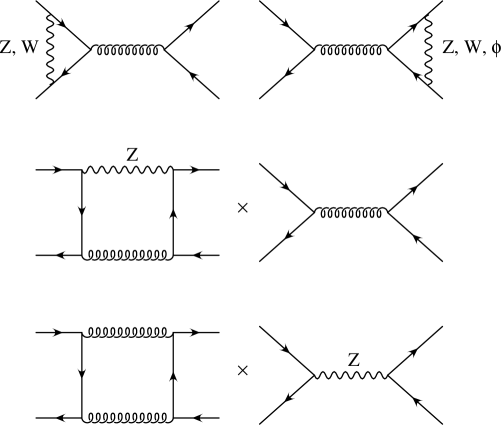
Figure III.1: Sample diagrams for the quark–antiquark annihilation process at ${\rm O}(\alpha_{s}^{2}\alpha)$.

The initial-state vertex corrections for $q\bar{q}\rightarrow b\bar{b}$ read

$$\overline{\sum}\left|{{\cal M}}^{V(q\bar{q}\rightarrow b\bar{b})}_{{\rm initial}}\right|^{2} = -\overline{\sum}\left|{{\cal M}}^{q\bar{q}\rightarrow b\bar{b}}_{{\alpha_{s}^{2}}}\right|^{2}$$ (III.10)

$$\times {\alpha\over 2\pi}\Bigg{[}{1\over 2}({g_{v}^{q}}^{2}+{g_{a}^{q}}^{2})\*f_{1}\left({{m_{Z}}^{2}\over s}\right)+{g_{W}}^{2}\*f_{1}\left({{m_{W}}^{2}\over s}\right)\Bigg{]}$$

with

$$f_{1}(x)=1+2\*\Big{[}\big{(}1+\ln(x)\big{)}\*\big{(}2\*x+3\big{)}-2\*\big{(}1+x\big{)}^{2}\Big{(}\mbox{Li}_{2}\left(1+{1\over x}\right)-{\pi^{2}\over 6}\Big{)}\Big{]}$$

and the squared leading order matrix element is given in Eq. (II.9). The final state vertex corrections read

$$\overline{\sum}\left|{{\cal M}}^{V_{Z}(q\bar{q}\rightarrow b\bar{b})}_{{\rm final}}\right|^{2}=-\overline{\sum}\left|{{\cal M}}^{q\bar{q}\rightarrow b\bar{b}}_{{\alpha_{s}^{2}}}\right|^{2}{\alpha\over 4\pi}\*({g_{v}^{b}}^{2}+{g_{a}^{b}}^{2})\*f_{1}\left({{m_{Z}}^{2}\over s}\right),$$ (III.11)

$$\overline{\sum}\left|{{\cal M}}^{V_{W}(q\bar{q}\rightarrow b\bar{b})}_{{\rm final}}\right|^{2} = \overline{\sum}\left|{{\cal M}}^{q\bar{q}\rightarrow b\bar{b}}_{{\alpha_{s}^{2}}}\right|^{2}\*{\alpha\over\pi}\*{g_{W}}^{2}$$ (III.12)

$$\times \*\Bigg{\{}-1+{2\*{m_{t}}^{2}-2\*{m_{W}}^{2}-3\*s\over s}$$

$$\times \bigg{(}{1\over{m_{t}}^{2}-{m_{W}}^{2}}\*\left({\overline{\rm A}_{0}({m_{W}}^{2})}-{\overline{\rm A}_{0}({m_{t}}^{2})}\right)+\*{\overline{\rm B}_{0}(s,{m_{t}}^{2},{m_{t}}^{2})}\bigg{)}$$

$$- {2\over s}\*\bigg{(}({m_{t}}^{2}-{m_{W}}^{2})^{2}+s\*(s-{m_{t}}^{2}+2\*{m_{W}}^{2})\bigg{)}\*{\rm C}_{0}(s,{m_{t}}^{2},{m_{W}}^{2},{m_{t}}^{2})$$

$$- ({m_{t}}^{2}-{m_{W}}^{2})\*{{\partial\over\partial p^{2}}{\rm B}_{0}(p^{2},{m_{t}}^{2},{m_{W}}^{2})\Big{|}_{p^{2}=0}}\Bigg{\}},$$

$$\overline{\sum}\left|{{\cal M}}^{V_{\phi}(q\bar{q}\rightarrow b\bar{b})}_{{\rm final}}\right|^{2} = \overline{\sum}\left|{{\cal M}}^{q\bar{q}\rightarrow b\bar{b}}_{{\alpha_{s}^{2}}}\right|^{2}\*{\alpha\over\pi}\*{g_{W}}^{2}\*{{m_{t}}^{2}\over 2{m_{W}}^{2}}$$ (III.13)

$$\times \*\Bigg{\{}-1+{2\*{m_{t}}^{2}-2\*{m_{W}}^{2}+s\over s}$$

$$\times \bigg{(}{1\over{m_{t}}^{2}-{m_{W}}^{2}}\*\left({\overline{\rm A}_{0}({m_{W}}^{2})}-{\overline{\rm A}_{0}({m_{t}}^{2})}\right)+\*{\overline{\rm B}_{0}(s,{m_{t}}^{2},{m_{t}}^{2})}\bigg{)}$$

$$- {2\over s}\*\bigg{(}({m_{t}}^{2}-{m_{W}}^{2})^{2}+s\*{m_{t}}^{2}\bigg{)}\*{\rm C}_{0}(s,{m_{t}}^{2},{m_{W}}^{2},{m_{t}}^{2})$$

$$- ({m_{t}}^{2}-{m_{W}}^{2})\*{{\partial\over\partial p^{2}}{\rm B}_{0}(p^{2},{m_{t}}^{2},{m_{W}}^{2})\Big{|}_{p^{2}=0}}\Bigg{\}},$$

where the scalar integrals are defined in the Appendix A. For the box-diagrams we find

$$\overline{\sum}\left|{{\cal M}}^{\Box{(q\bar{q}\rightarrow b\bar{b})}}_{\rm QCD}\right|^{2} = 4\*\pi\*\alpha\*\alpha_{s}^{2}\*{s\over s-{m_{Z}}^{2}}\*{N^{2}-1\over N^{2}}\*$$ (III.14)

$$\times \Bigg{\{}{g_{v}^{q}}\*{g_{v}^{b}}\*\Big{[}\ln\left({t\over u}\right)-z\*\ln\left({t\*u\over s^{2}}\right)$$

$$+ (1+z+z^{2})\*\ln^{2}\left(-{t\over s}\right)-(1-z+z^{2})\*\ln^{2}\left(-{u\over s}\right)\Big{]}$$

$$+ {g_{a}^{q}}\*{g_{a}^{b}}\*\Big{[}z\*\ln\left({u\over t}\right)+\ln\left({t\*u\over s^{2}}\right)$$

$$- z\*\ln^{2}\left(-{t\over s}\right)+z\*\ln^{2}\left(-{u\over s}\right)\Big{]}\Bigg{\}}$$

$$+ \*\pi\*\alpha\*\alpha_{s}^{2}\*{N^{2}-1\over N^{2}}\*{\rm B}^{q\bar{q}\rightarrow b\bar{b}}\*\Bigg{\{}(4\pi)^{\varepsilon}\Gamma(1+\varepsilon)\Big{[}{1\over\varepsilon}\ln\left({t\over u}\right)$$

$$+ {1\over 2}\ln^{2}\left({\mu^{2}\over-u}\right)-{1\over 2}\ln^{2}\left({\mu^{2}\over-t}\right)\Big{]}\Bigg{\}},$$

$$\overline{\sum}\left|{{\cal M}}^{\Box{(q\bar{q}\rightarrow b\bar{b})}}_{\rm EW}\right|^{2} = 4\*\pi\alpha\*\alpha_{s}^{2}\*{N^{2}-1\over N^{2}}$$ (III.15)

$$\times \Bigg{\{}{g_{v}^{q}}{g_{v}^{b}}\Bigg{[}2\*\ln\left({t\over u}\right)$$

$$- 2\*z\*\bigg{[}\ln\left({tu\over{m_{Z}}^{4}}\right)-2\*{s-{m_{Z}}^{2}\over s}\*\ln\left(\left|1-{s\over{m_{Z}}^{2}}\right|\right)-4\*\mbox{Li}_{2}\left(1-{s\over{m_{Z}}^{2}}\right)\bigg{]}$$

$$- 4\*\bigg{[}\Big{(}{s\*(1+z^{2})\over s-{m_{Z}}^{2}}-{{m_{Z}}^{2}\over s}\Big{)}\*\ln\left(1-{s\over{m_{Z}}^{2}}\right)\ln\left({t\over u}\right)$$

$$- z\*\ln\left(1-{s\over{m_{Z}}^{2}}\right)\ln\left({s^{2}\over tu}\right)\bigg{]}$$

$$- 2\*\bigg{[}\Big{(}{s\*(1+z^{2})\over s-{m_{Z}}^{2}}-{2\*{m_{Z}}^{2}\over s}\Big{)}\*\left(\mbox{Li}_{2}\left(1+{t\over{m_{Z}}^{2}}\right)-\mbox{Li}_{2}\left(1+{u\over{m_{Z}}^{2}}\right)\right)$$

$$+ 2\*z\*\left(\mbox{Li}_{2}\left(1+{u\over{m_{Z}}^{2}}\right)+\mbox{Li}_{2}\left(1+{t\over{m_{Z}}^{2}}\right)\right)\bigg{]}\Bigg{]}$$

$$+ {g_{a}^{b}}\*{g_{a}^{q}}\Bigg{[}2\*\ln\left({tu\over{m_{Z}}^{4}}\right)-2\*z\ln\left({t\over u}\right)-4\*{s-{m_{Z}}^{2}\over s}\*\ln\left(\left|1-{s\over{m_{Z}}^{2}}\right|\right)$$

$$+ {4{m_{Z}}^{2}\over s}\bigg{[}\mbox{Li}_{2}\left(1+{t\over{m_{Z}}^{2}}\right)+\mbox{Li}_{2}\left(1+{u\over{m_{Z}}^{2}}\right)-2\*\mbox{Li}_{2}\left(1-{s\over{m_{Z}}^{2}}\right)$$

$$- \ln\left(1-{s\over{m_{Z}}^{2}}\right)\ln\left({s^{2}\over tu}\right)\bigg{]}$$

$$+ 4\*z\*{s+{m_{Z}}^{2}\over s-{m_{Z}}^{2}}\ln\left(1-{s\over{m_{Z}}^{2}}\right)\ln\left({t\over u}\right)$$

$$+ {4\*{m_{Z}}^{2}\over s-{m_{Z}}^{2}}\*z\*\bigg{[}\mbox{Li}_{2}\left(1+{t\over{m_{Z}}^{2}}\right)-\mbox{Li}_{2}\left(1+{u\over{m_{Z}}^{2}}\right)\bigg{]}\Bigg{]}\Bigg{\}}$$

$$+ \pi\*\alpha\*\alpha_{s}^{2}\*{N^{2}-1\over N^{2}}\*{\rm B}^{q\bar{q}\rightarrow b\bar{b}}\*\Bigg{\{}(4\pi)^{\varepsilon}\Gamma(1+\varepsilon)\Big{[}{1\over\varepsilon}\ln\left({t\over u}\right)$$

$$+ {1\over 2}\ln^{2}\left({\mu^{2}\over-u}\right)-{1\over 2}\ln^{2}\left({\mu^{2}\over-t}\right)\Big{]}\Bigg{\}},$$

with

$${\rm B}^{q\bar{q}\rightarrow b\bar{b}} = {8\*s\over s-{m_{Z}}^{2}}\*\Big{(}(d-3+z^{2})\*{g_{v}^{q}}\*{g_{v}^{b}}-z\*(d-2)\*(d-3)\*{g_{a}^{q}}\*{g_{a}^{b}}\Big{)}.$$ (III.16)

The factor ${\rm B}^{q\bar{q}\rightarrow b\bar{b}}$ results from the interference between the leading order QCD amplitude and the weak amplitude. Terms proportional to the $Z$ vector couplings are odd functions in the scattering angle $z$ as a consequence of Furry’s theorem. The virtual corrections for the remaining quark-induced processes can be deduced by the crossing relations Eq. (II.3). For latter use we extract the IR divergent contribution to the differential cross section

$${{\rm d}\sigma_{q\bar{q}\rightarrow b\bar{b}}^{\Box\>\>\rm IR}\over{\rm d}z}={\alpha\*\alpha_{s}^{2}\over 32s}\*{N^{2}-1\over N^{2}}\*{\rm B}^{q\bar{q}\rightarrow b\bar{b}}\*\Bigg{\{}(4\pi)^{\varepsilon}\Gamma(1+\varepsilon)\Big{[}{2\over\varepsilon}\ln\left({t\over u}\right)+\ln^{2}\left({\mu^{2}\over-u}\right)-\ln^{2}\left({\mu^{2}\over-t}\right)\Big{]}\Bigg{\}}.$$ (III.17)

The contribution from real emission is given by

$$\overline{\sum}\left|{{\cal M}}^{q\bar{q}\rightarrow b\bar{b}g}\right|^{2} = \alpha_{s}^{2}\*\alpha\*(4\*\pi)^{3}\>\*{N^{2}-1\over N^{2}}$$

$$\times \Big{(}{g_{v}^{q}}\*{g_{v}^{b}}\*(t_{1}^{2}+t_{2}^{2}+u_{1}^{2}+u_{2}^{2})-{g_{a}^{q}}\*{g_{a}^{b}}\*(t_{1}^{2}+t_{2}^{2}-u_{1}^{2}-u_{2}^{2})\Big{)}$$

$$\times {1\over s}\>\>\*{1\over s-{m_{Z}}^{2}}\>\>\*{1\over s+t_{1}+t_{2}+u_{1}+u_{2}}\>\>\*{1\over s+t_{1}+t_{2}+u_{1}+u_{2}+{m_{Z}}^{2}}$$

$$\times {1\over s+t_{1}+u_{1}}\>\>\*{1\over s+t_{2}+u_{1}}\>\>\*{1\over s+t_{1}+u_{2}}\>\>\*{1\over s+t_{2}+u_{2}}$$

$$\times \Big{(}2\*s^{2}+(t_{1}+t_{2}+u_{1}+u_{2})\*(2\*s-{m_{Z}}^{2})\Big{)}$$

$$\times \Big{(}(t_{1}+t_{2}-u_{1}-u_{2})\*s^{2}+((t_{1}+t_{2})^{2}-(u_{1}+u_{2})^{2})\*s$$

$$+ (t_{1}+t_{2}+u_{1}+u_{2})\*(t_{1}\*t_{2}-u_{1}\*u_{2})\Big{)}$$

with

$$t_{1} = -2k_{q}k_{b},\quad t_{2}=-2k_{\bar{q}}k_{\bar{b}},$$

$$u_{1} = -2k_{q}k_{\bar{b}},\quad u_{2}=-2k_{\bar{q}}k_{b}.$$ (III.19)

The combination $s+t_{1}+t_{2}+u_{1}+u_{2}+{m_{Z}}^{2}$ appearing in Eq. (LABEL:eq:real-qqb) can vanish, corresponding to on-shell production of the $Z$ boson. Therefore we introduced according to the principal value prescription a cut around the singular point

$$\delta>\sqrt{|s+t_{1}+t_{2}+u_{1}+u_{2}+{m_{Z}}^{2}|}.$$

and demonstrated numerically that the result remains unchanged for $\delta$ between $10^{-1}$ and $10^{-5}$ GeV. Moreover we checked that also a fictitious $Z$ boson width $0.01\>\>{\rm GeV}\leq\Gamma_{Z}\leq 1\>\>{\rm GeV}$ produces the same numerical result. In analogy with the leading-order crossing relations we find for the remaining real corrections:

$$\overline{\sum}\left|{{\cal M}}^{q\bar{b}\rightarrow q\bar{b}g}\right|^{2}=\overline{\sum}\left|{{\cal M}}^{\bar{q}b\rightarrow\bar{q}bg}\right|^{2}=\overline{\sum}\left|{{\cal M}}^{q\bar{q}\rightarrow b\bar{b}g}\right|^{2}\Bigg{|}_{s\leftrightarrow t_{1},\>\>t_{2}\rightarrow-s-t_{1}-t_{2}-u_{1}-u_{2}},$$ (III.20)

$$\overline{\sum}\left|{{\cal M}}^{qb\rightarrow qbg}\right|^{2} = \overline{\sum}\left|{{\cal M}}^{\bar{q}\bar{b}\rightarrow\bar{q}\bar{b}g}\right|^{2}$$

$$= \overline{\sum}\left|{{\cal M}}^{q\bar{b}\rightarrow q\bar{b}g}\right|^{2}\Big{|}_{s\leftrightarrow u_{2},\>\>u_{1}\rightarrow-s-t_{1}-t_{2}-u_{2}-u_{1}}$$

$$= \overline{\sum}\left|{{\cal M}}^{q\bar{q}\rightarrow b\bar{b}g}\right|^{2}\Bigg{|}_{s\rightarrow t_{1},\>\>t_{1}\rightarrow u_{1},\>\>t_{2}\rightarrow u_{2},\>\>u_{1}\rightarrow s,\>\>u_{2}\rightarrow-s-t_{1}-t_{2}-u_{1}-u_{2}}.$$

For these contributions the $Z$ boson remains off-shell. To get an infrared finite result the corresponding subtraction terms from the dipole formalism were implemented. We checked explicitly the numerical stability of real corrections and dipoles and found the pointwise cancellation between the two contributions in the singular phase space regions. However the dipoles approximate the real corrections very well also in non-singular regions. This results in large cancellations in the integrated result. In contrast to the singular configurations this cancellation is not pointwise but takes place between different phase space regions. As a consequence of this behaviour one needs high statistics for the numerical integration. To check the numerical results we therefore implemented also a variant of the phase-space-slicing method [2] and find agreement comparing the results of both methods. The relevant formulae for the slicing method and the plot for the comparison are shown in the Appendix B.

Let us now come to the contributions from the dipole formalism ${\bf F}\otimes{\rm d}\sigma^{{\rm B}}$ with ${\bf F}={\bf I,K,P}$. The symbol ‘$\otimes$’ denotes spin and colour correlation between the operator ${\bf F}$ and the leading order amplitudes, which are treated in general as vectors in colour and spin space. For the processes under consideration, the gluon is always emitted from a fermion line and only trivial spin correlation appears. We start with the contribution for the quark–antiquark annihilation channel

$$\left({\bf I}\otimes{\rm d}\sigma^{{\rm B}}\right)^{q\bar{q}\rightarrow b\bar{b}} = -{\alpha\alpha_{s}^{2}\over 32s}\*{N^{2}-1\over N^{2}}{{\rm B}^{q\bar{q}\rightarrow b\bar{b}}}\Bigg{\{}{(4\pi)^{\varepsilon}\over\Gamma(1-\varepsilon)}\*\Big{[}{2\over\varepsilon}\*\ln\left({t\over u}\right)$$

$$+ \ln^{2}\left({\mu^{2}\over-u}\right)-\ln^{2}\left({\mu^{2}\over-t}\right)+3\ln\left({t\over u}\right)\Big{]}\Bigg{\}},$$

(III.22)

where ${{\rm B}^{q\bar{q}\rightarrow b\bar{b}}}$ is defined in Eq. (III.16). This contribution to the differential cross section cancells the IR-poles and the $\mu$-dependence from the virtual corrections in Eq. (III.17). For the finite ${\bf K}$ and ${\bf P}$ parts we find

$$\left({\bf K}\otimes{\rm d}\sigma^{{\rm B}}\right)^{q\bar{q}\rightarrow b\bar{b}}(x) = 0,$$ (III.23)

$$\left({\bf P}\otimes{\rm d}\sigma^{{\rm B}}\right)^{q\bar{q}\rightarrow b\bar{b}}(x) = {\alpha\alpha_{s}^{2}\over 32sx}\*{N^{2}-1\over N^{2}}{{\rm B}^{q\bar{q}\rightarrow b\bar{b}}}\*\ln\left({t\over u}\right)\left({1+x^{2}\over 1-x}\right)_{+}.$$ (III.24)

Of course in Eq. (III.24) ${{\rm B}^{q\bar{q}\rightarrow b\bar{b}}}$ is also a function of $x$ and for the evaluation of the plus distribution the well known relation

$$\int_{0}^{1}{\rm d}x\Big{(}f(x)\Big{)}_{+}g(x)=\int^{1}_{0}{\rm d}x\>f(x)\>[g(x)-g(1)]$$ (III.25)

is used. For $\bar{b}q\rightarrow\bar{b}q$ and $b\bar{q}\rightarrow b\bar{q}$ we find

$$\left({\bf I}\otimes{\rm d}\sigma^{{\rm B}}\right)^{\bar{b}q\rightarrow\bar{b}q} = \left({\bf I}\otimes{\rm d}\sigma^{{\rm B}}\right)^{b\bar{q}\rightarrow b\bar{q}}$$

$$= -{\alpha\alpha_{s}^{2}\over 32s}\*{N^{2}-1\over N^{2}}{{\rm B}^{\bar{b}q\rightarrow\bar{b}q}}\Bigg{\{}{(4\pi)^{\varepsilon}\over\Gamma(1-\varepsilon)}\*\Big{[}{2\over\varepsilon}\*\ln\left({s\over-u}\right)$$

$$+ \ln^{2}\left({\mu^{2}\over-u}\right)-\ln^{2}\left({\mu^{2}\over s}\right)+3\ln{\left({s\over-u}\right)}\Big{]}\Bigg{\}},$$

(III.26)

$$\left({\bf K}\otimes{\rm d}\sigma^{{\rm B}}\right)^{\bar{b}q\rightarrow\bar{b}q}(x) = \left({\bf K}\otimes{\rm d}\sigma^{{\rm B}}\right)^{b\bar{q}\rightarrow b\bar{q}}(x)$$ (III.27)

$$= {\alpha\alpha_{s}^{2}\over 32sx}\*{N^{2}-1\over N^{2}}{{\rm B}^{\bar{b}q\rightarrow\bar{b}q}}\*\Bigg{[}\delta(1-x)\*\left({3\over 2}-{\pi^{2}\over 3}\right)-(1+x)\*\ln(1-x)$$

$$+ {3\over 2}\left({1\over 1-x}\right)_{+}+\left({2\ln(1-x)\over 1-x}\right)_{+}\Bigg{]},$$

$$\left({\bf P}\otimes{\rm d}\sigma^{{\rm B}}\right)^{\bar{b}q\rightarrow\bar{b}q}(x) = \left({\bf P}\otimes{\rm d}\sigma^{{\rm B}}\right)^{b\bar{q}\rightarrow b\bar{q}}(x)$$ (III.28)

$$= -{\alpha\alpha_{s}^{2}\over 32sx}\*{N^{2}-1\over N^{2}}{{\rm B}^{\bar{b}q\rightarrow\bar{b}q}}\*\ln\left({-u\over s}\right)\left({1+x^{2}\over 1-x}\right)_{+},$$

where ${\rm B}^{\bar{b}q\rightarrow\bar{b}q}$ can be deduced from ${\rm B}^{q\bar{q}\rightarrow b\bar{b}}$ and Eq. (II.3). For $\bar{b}\bar{q}\rightarrow\bar{b}\bar{q}$ (and $bq\rightarrow bq$) we find

$$\left({\bf I}\otimes{\rm d}\sigma^{{\rm B}}\right)^{\bar{b}\bar{q}\rightarrow\bar{b}\bar{q}} = \left({\bf I}\otimes{\rm d}\sigma^{{\rm B}}\right)^{bq\rightarrow bq}$$

$$= {\alpha\alpha_{s}^{2}\over 32s}\*{N^{2}-1\over N^{2}}{{\rm B}^{\bar{b}\bar{q}\rightarrow\bar{b}\bar{q}}}\Bigg{\{}{(4\pi)^{\varepsilon}\over\Gamma(1-\varepsilon)}\*\Big{[}{2\over\varepsilon}\*\ln\left({s\over-u}\right)$$

$$+ \ln^{2}\left({\mu^{2}\over-u}\right)-\ln^{2}\left({\mu^{2}\over s}\right)+3\ln{\left({s\over-u}\right)}\Big{]}\Bigg{\}},$$

$$\left({\bf K}\otimes{\rm d}\sigma^{{\rm B}}\right)^{\bar{b}\bar{q}\rightarrow\bar{b}\bar{q}}(x) = \left({\bf K}\otimes{\rm d}\sigma^{{\rm B}}\right)^{bq\rightarrow bq}(x)$$ (III.30)

$$= -{\alpha\alpha_{s}^{2}\over 32sx}\*{N^{2}-1\over N^{2}}{{\rm B}^{\bar{b}\bar{q}\rightarrow\bar{b}\bar{q}}}\*\Bigg{[}\delta(1-x)\*\left({3\over 2}-{\pi^{2}\over 3}\right)-(1+x)\*\ln(1-x)$$

$$+ {3\over 2}\left({1\over 1-x}\right)_{+}+\left({2\ln(1-x)\over 1-x}\right)_{+}\Bigg{]},$$

$$\left({\bf P}\otimes{\rm d}\sigma^{{\rm B}}\right)^{\bar{b}\bar{q}\rightarrow\bar{b}\bar{q}}(x) = \left({\bf P}\otimes{\rm d}\sigma^{{\rm B}}\right)^{bq\rightarrow bq}(x)$$ (III.31)

$$= {\alpha\alpha_{s}^{2}\over 32sx}\*{N^{2}-1\over N^{2}}{{\rm B}^{\bar{b}\bar{q}\rightarrow\bar{b}\bar{q}}}\*\ln\left({-u\over s}\right)\left({1+x^{2}\over 1-x}\right)_{+},$$

and ${\rm B}^{\bar{b}\bar{q}\rightarrow\bar{b}\bar{q}}$ is obtained by the crossing relations Eq. (II.3) as above.

III.2 Weak corrections to gluon-induced processes

Sample diagrams for the virtual corrections to the gluon-induced processes are shown in Fig III.2. No infrared divergencies are present and no corrections from real radiation contribute. The weak corrections are again classified into those from self-energy-, vertex- and box-diagrams. The latter are UV finite, vertex and self-energy contributions must be renormalized. The differential cross section for the gluon fusion channel at next-to-leading order is decomposed as follows:

$${{\rm d}\sigma^{{\rm O}(\alpha_{s}^{2}\alpha)gg\rightarrow b\bar{b}}\over{\rm d}z} = {1\over 32\pi s}\sum_{i=Z,W,\phi}\Bigg{[}\overline{\sum}|{{\cal M}}^{\Box_{i}(gg\rightarrow b\bar{b})}|^{2}+\overline{\sum}|{{\cal M}}^{V_{i}(gg\rightarrow b\bar{b})}|^{2}$$ (III.32)

$$+ \overline{\sum}|{{\cal M}}^{\Sigma_{i}(gg\rightarrow b\bar{b})}|^{2}\Bigg{]}.$$

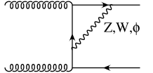
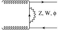
Figure III.2: Sample diagrams for the gluon fusion process at ${\rm O}(\alpha_{s}^{2}\alpha)$.

We start with the analytic results for the self-energy diagrams (Fig III.2(c)) in the $gg\rightarrow b\bar{b}$ channel, which can be written in a compact form

$$\overline{\sum}|{{\cal M}}^{\Sigma_{Z}(gg\rightarrow b\bar{b})}|^{2} = \pi\*\alpha_{s}^{2}\alpha\*\Bigg{\{}{2-N^{2}+N^{2}z\over N(N^{2}-1)\*s}({g_{v}^{b}}^{2}+{g_{a}^{b}}^{2}){1+z^{2}\over(1+z)^{2}}\*\Big{[}3\*s\*(1+z)+4\*{m_{Z}}^{2}$$

$$- {2\over s\*(1+z)}\*\Big{(}s\*(1+z)+2\*{m_{Z}}^{2}\Big{)}^{2}\*\ln\left(1+{s\*(1+z)\over 2\*{m_{Z}}^{2}}\right)\Big{]}+(z\rightarrow-z)\Bigg{\}},$$

$$\overline{\sum}|{{\cal M}}^{\Sigma_{W}(gg\rightarrow b\bar{b})}|^{2} = 4\*\pi\*\alpha_{s}^{2}\alpha\*\Bigg{\{}\*{2-N^{2}+N^{2}z\over N(N^{2}-1)\*s}{g_{W}}^{2}{1+z^{2}\over(1+z)^{2}}\*$$ (III.34)

$$\times \Bigg{[}{1\over 2\*({m_{t}}^{2}-{m_{W}}^{2})}\*\Big{(}s\*(1+z)\*({m_{t}}^{2}-3\*{m_{W}}^{2})-4\*({m_{t}}^{2}-{m_{W}}^{2})^{2}\Big{)}$$

$$+ {{m_{W}}^{2}\over({m_{t}}^{2}-{m_{W}}^{2})^{2}}\*\Big{(}s\*(1+z)\*(2\*{m_{t}}^{2}-{m_{W}}^{2})$$

$$- 2\*({m_{t}}^{2}-{m_{W}}^{2})^{2}\Big{)}\*\ln\left({{m_{t}}^{2}\over{m_{W}}^{2}}\right)$$

$$+ \left(s\*(1+z)+2{m_{W}}^{2}-2{m_{t}}^{2}\right)\*f(y_{1},y_{2})\Bigg{]}+(z\rightarrow-z)\Bigg{\}},$$

where

$$f(y_{1},y_{2})=-y_{1}\*\ln\left({y_{1}\over y_{1}-1}\right)-y_{2}\*\ln\left({y_{2}\over y_{2}-1}\right)$$ (III.35)

$$y_{1/2} = {t+{m_{W}}^{2}-{m_{t}}^{2}\over 2t}\*\times\left(1\pm\sqrt{1-{4{m_{W}}^{2}t\over(t+{m_{W}}^{2}-{m_{t}}^{2})^{2}}}\right).$$

The contributions involving $\phi$ and $W$ are closely related

$$\overline{\sum}|{{\cal M}}^{\Sigma_{\phi}(gg\rightarrow b\bar{b})}|^{2}={{m_{t}}^{2}\over 2\*{m_{W}}^{2}}\*\overline{\sum}|{{\cal M}}^{\Sigma_{W}(gg\rightarrow b\bar{b})}|^{2}.$$ (III.37)

The vertex corrections consist of $s$, $t$ and $u$ channel contributions. Since the corrections to the $s$ channel are proportional to the quark mass (see Ref. [12] Eqs.(II.18-22)) they vanish in the massless limit. The remaining vertex corrections (e.g. Fig. III.2(b)) can be expressed in terms of the self energies

$$\overline{\sum}|{{\cal M}}^{V_{i}(gg\rightarrow b\bar{b})}|^{2}=-2\overline{\sum}|{{\cal M}}^{\Sigma_{i}(gg\rightarrow b\bar{b})}|^{2}.$$ (III.38)

The box contributions (Fig III.2(a)) are more involved and are listed in Appendix C. Corrections to $gb\rightarrow gb$ and $g\bar{b}\rightarrow g\bar{b}$ are obtained via the relations Eq. (II.4).

IV Results

Apart of the obvious checks, like cancelation of UV and IR singularities, a numerical test was performed for the IR-divergent contributions, implementing the phase-space-slicing method. As illustrated in Appendix B we found complete agreement of the two methods. For the quark-antiquark annihilation and the gluon fusion channel we found complete analytical agreement with previous results for top-quark production [12], with the following replacements

$${m_{t}}\leftrightarrow{m_{b}},\quad{g_{v}^{t}}\rightarrow{g_{v}^{b}},\quad{g_{a}^{t}}\rightarrow{g_{a}^{b}}\quad{\rm and}\quad{{m_{t}}\rightarrow 0}.$$

These results also allow for a numerical comparison between the massive and the massless approach. In Fig. IV.1 the results for a massive bottom-quark (${m_{b}}=4.82$ GeV) are compared with those from the massless approximation. Agreement between the massive and the massless results is observed in the full kinematic range, which justifies the massless approximation for the bottom-quarks used in the paper. The difference of the massless and the massive result concerning the relative corrections is always below $0.5\%$. Furthermore all LO and NLO partonic corrections were calculated analytically and thus all crossing relations listed in the previous Sections are used as additional cross check. For the numerical evaluation we use the same input parameters as in Section II. As mentioned in Section III the results are leading order in QCD and therefore evaluated with the leading order PDF’s CTEQ6L.
We start with the results for the differential ${p_{\rm T}}$-distribution at the Tevatron. In Fig. IV.2 the relative corrections normalised to the full leading order cross section are shown.

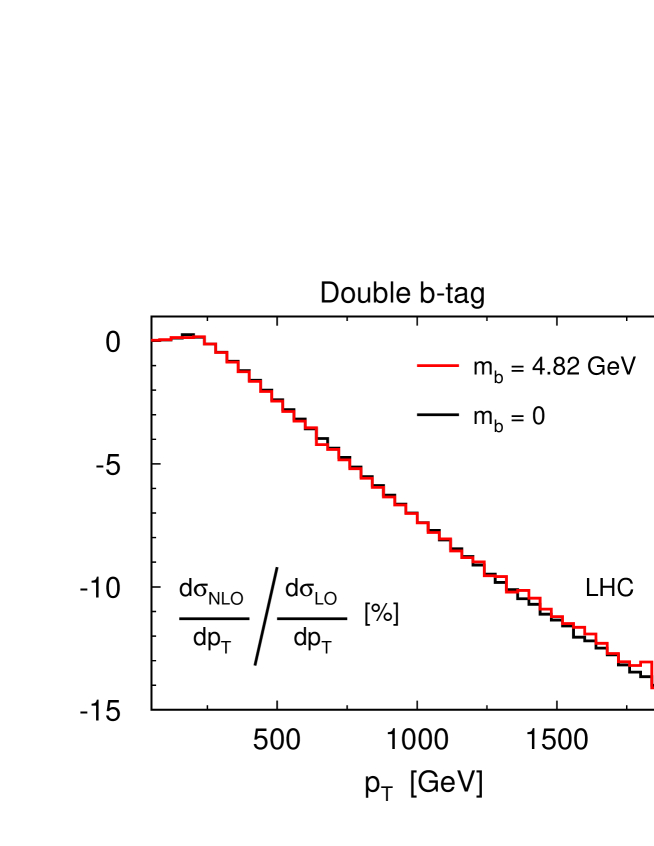
Figure IV.1: Relative weak corrections for double $b$-tag events at the LHC, comparing the results for a massless bottom-quark with the massive case.

Figure IV.2: Relative weak corrections for single $b$-tag (upper figure) and double $b$-tag events (lower figure) at the Tevatron.

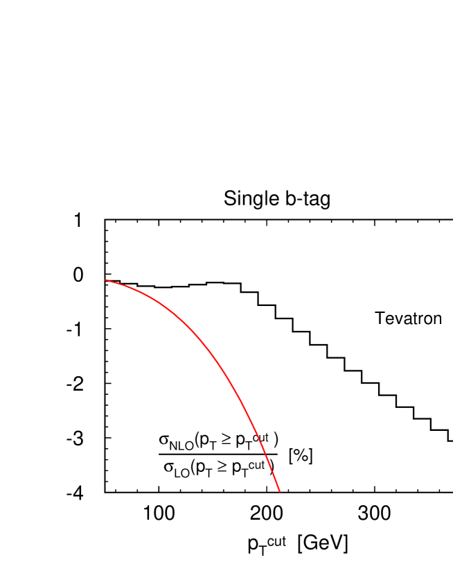
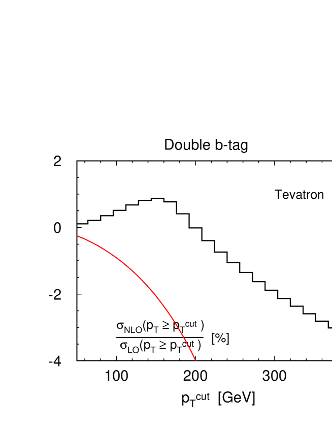
Figure IV.3: Relative corrections to the cross section for ${p_{\rm T}}>p_{\rm T}^{\rm cut}$ at the Tevatron for single $b$-tag (upper figure) and double $b$-tag events (lower figure). The red lines give an estimate on the statistical uncertainty as described in the text.

For single $b$-tag events (upper figure) the relative corrections are negative and of the order of a few permille up to ${p_{\rm T}}=120$ GeV. The following increase of the relative corrections with the resonant behaviour around ${p_{\rm T}}=180$ GeV is caused by the vertex corrections to $q\bar{q}\rightarrow b\bar{b}$ involving virtual top-quarks. In this range of ${p_{\rm T}}$ the weak corrections become positive and increase the differential cross section by a few permille. Above the resonance peak the weak corrections become negative again and the typical Sudakov behaviour is observed. The magnitude of the relative corrections increases with energy for ${p_{\rm T}}>200$ GeV and reaches $-3\%$ for ${p_{\rm T}}=400$ GeV.
Due to the aforementioned virtual top-quarks, the relative corrections for double $b$-tag events are positive for ${p_{\rm T}}$ values below 220 GeV (lower figure). In this case $q\bar{q}\rightarrow b\bar{b}$ and $gg\rightarrow b\bar{b}$ are the only contributing partonic channels, hence the resonance peak is more distinct than in the single $b$-tag case with the maximum ($+1.5\%$) of the relative corrections around ${p_{\rm T}}=180$ GeV. The influence of the Sudakov logarithms starts for ${p_{\rm T}}>220$ GeV, where the weak corrections change sign and become negative. For ${p_{\rm T}}=400$ GeV the relative corrections amount up to $-3\%$.
The relative corrections to the integrated cross section (${p_{\rm T}}>p_{\rm T}^{\rm cut}$) at the Tevatron are shown in Fig. IV.3. For the single $b$-tag (upper figure) and the double $b$-tag (lower figure) the peak around the $t\bar{t}$-threshold is smoothed by contributions from higher ${p_{\rm T}}$-values, leaving the integrated correction negative in the single $b$-tag case. Beyond ${p_{\rm T}}=200$ GeV the relative corrections to the integrated distributions are between $0$ and $-3\%$. In addition we give in Fig. IV.3 a rough estimate of the expected statistical error at the Tevatron. The estimated number of events for ${p_{\rm T}}>p_{\rm T}^{\rm cut}$ is based on an integrated luminosity of 8 ${\rm fb}^{-1}$. A comparison of the statistical uncertainty with the relative weak corrections shows that the weak effects will not be visible at the Tevatron.

At the LHC however the corrections are significantly larger. For the subsequent discsusion $\sqrt{s}=14$ TeV will be adopted. The relative corrections to the leading order ${p_{\rm T}}$-distributions are shown in Fig. IV.4. For single $b$-tag events (upper figure) the relative corrections are always negative and of the order of a few permille up to $-1\%$ for 50 GeV $<{p_{\rm T}}<$ 250 GeV. In contrast to the Tevatron results, the resonant behaviour arising from virtual top-quarks in quark–anti-quark annihilation is not visible, a consequence of the dominance of the gluon-induced processes in this ${p_{\rm T}}$-regime (Fig. II.4(a)). For 250 GeV $<{p_{\rm T}}<$ 1 TeV the weak NLO contributions vary between $-1\%$ and $-8\%$, compared to the leading order distribution, a consequence of the Sudakov logarithms. In the high energy regime (${p_{\rm T}}>1$ TeV) the relative corrections amount to $-10\%$ and will even reach $-14\%$ for ${p_{\rm T}}=2$ TeV.
The lower figure in Fig. IV.4 shows the relative corrections for double $b$-tag events at the LHC. Despite the strong suppression of $q\bar{q}\rightarrow b\bar{b}$ at leading order (see Fig. II.4(b)) a small remnant of the enhancement from virtual top-quarks is visible in the double $b$-tag case. With increasing ${p_{\rm T}}$ the Sudakov logarithms dominate the shape of the weak NLO contributions and yield relative corrections between $-1\%$ and $-7\%$ (250 GeV $<{p_{\rm T}}<$ 1 TeV). At the highest ${p_{\rm T}}$-values considered relative corrections up to $-14\%$ are observed.
Fig. IV.5 (upper figure) shows the integrated cross section for single $b$-tag events at the LHC together with an estimate of the statistical error based on an integrated luminosity of 200 ${\rm fb}^{-1}$. The same composition in shape and magnitude is observed as for the differential distribution. The statistical error estimate matches the size of the weak corrections up to ${p_{\rm T}}=1.5$ TeV. For higher ${p_{\rm T}}$-values the rate drops quickly and it will be difficult to observe the effect of the weak corrections. For double $b$-tag events (lower figure) we find again the smoothing of the $t\bar{t}$-threshold for the relative weak corrections, while the composition of the curve for ${p_{\rm T}}>250$ GeV is very similiar to the already discussed differential distribution. Considering the statistical error, the slight increase from virtual top-quarks will not be observable at the LHC. For ${p_{\rm T}}$-values between $250$-$1000$ GeV the weak corrections are larger than the statistical error, above ${p_{\rm T}}=1$ TeV they are comparable or smaller.
In Fig. IV.6 we show results for the LHC operating at $\sqrt{s}=10$ TeV. The absolute cross sections are by more than a factor two lower, due to the lower parton luminosities. However the impact of the electroweak corrections is nearly the same and qualitatively similiar results are obtained for the relative NLO corrections.

Figure IV.4: Relative weak corrections for single $b$-tag (upper figure) and double $b$-tag (lower figure) events at the LHC.

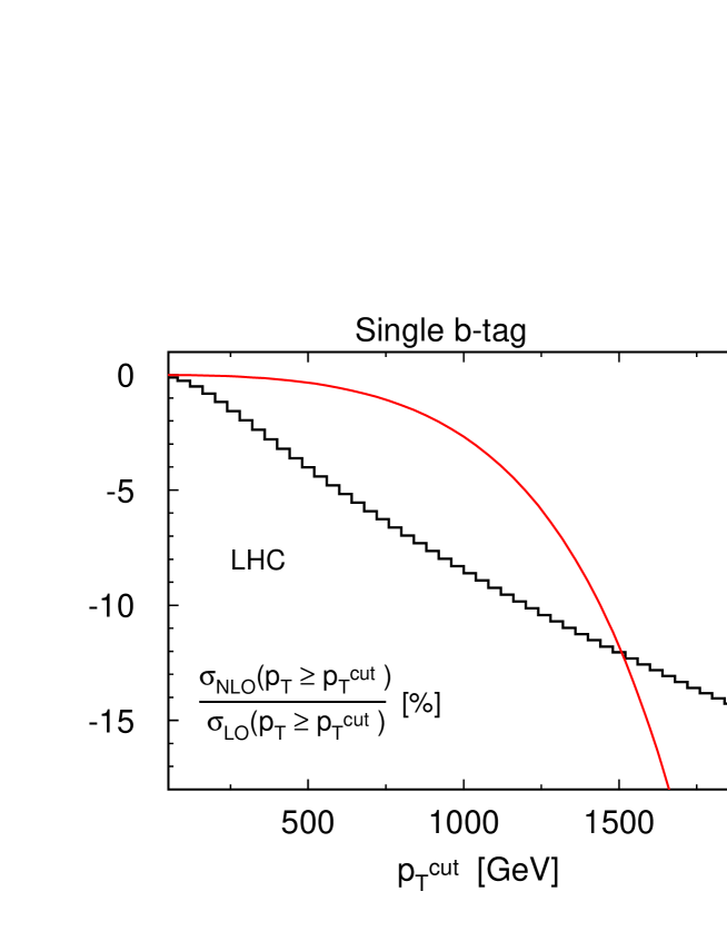
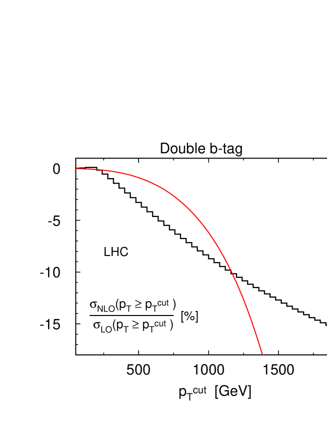
Figure IV.5: Relative corrections to the cross section for ${p_{\rm T}}>p_{\rm T}^{\rm cut}$ at the LHC for single $b$-tag (upper figure) and double $b$-tag events (lower figure). The red lines give an estimate on the statistical uncertainty as described in the text.

Figure IV.6: Relative corrections for single $b$-tag (a) and double $b$-tag events (b) at the LHC operating with a center-of-mass energy $\sqrt{s}=10$ TeV (upper figures) and the ratio of the differential leading order cross sections at the LHC operating at 10 TeV and 14 TeV $\left({\rm d}\sigma_{\rm LO}(10\>{\rm TeV})/{\rm d}{p_{\rm T}}\right)/\left({\rm d}\sigma_{\rm LO}(14\>{\rm TeV})/{\rm d}{p_{\rm T}}\right)$ (lower figures).

V Conclusion

In this article we present the weak corrections for $b$-jet production of order ${\alpha_{s}^{2}\alpha}$ neglecting purely photonic corrections. We derive compact analytic results for the NLO contributions in quark–anti-quark annihilation and the gluon-fusion. For the remaining partonic processes we list the crossing relations needed to derive the corresponding analytic results. We present the corrections to the ${p_{\rm T}}$-distribution and compare the results with the expected statistical uncertainty. In particular we find corrections up to ten percent for bottom-jets at high transverse momenta accessible at the LHC. These effects are larger than the anticipated statistical uncertainty.

Acknowledgements: This work is supported by the European Community’s Marie-Curie Research Training Network under contract MRTN-CT-2006-035505 “Tools and Precision Calculations for Physics Discoveries at Colliders”. P.U. acknowledges the support of the Initiative and Networking Fund of the Helmholtz Association, contract HA-101 (“Physics at the Terascale”).

Appendix A Notation

We define as usual

$${\rm A}_{0}({m_{1}}^{2})={1\over i\pi^{2}}\int{\rm d}^{d}\ell{(2\pi\mu)^{2\varepsilon}\over(\ell^{2}-{m_{1}}^{2}+i\varepsilon)}$$

$${\rm B}_{0}(p_{1}^{2},{m_{1}}^{2},{m_{2}}^{2})={1\over i\pi^{2}}\int{\rm d}^{d}\ell{(2\pi\mu)^{2\varepsilon}\over(\ell^{2}-{m_{1}}^{2}+i\varepsilon)((\ell+p_{1})^{2}-{m_{2}}^{2}+i\varepsilon)},$$

$${\rm C}_{0}(p_{1}^{2},p_{2}^{2},(p_{1}+p_{2})^{2},{m_{1}}^{2},{m_{2}}^{2},{m_{3}}^{2})=$$

$${1\over i\pi^{2}}\int{\rm d}^{d}\ell{(2\pi\mu)^{2\varepsilon}\over(\ell^{2}-{m_{1}}^{2}+i\varepsilon)((\ell+p_{1})^{2}-{m_{2}}^{2}+i\varepsilon)((\ell+p_{1}+p_{2})^{2}-{m_{3}}^{2}+i\varepsilon)},$$

$${\rm D}_{0}(p_{1}^{2},p_{2}^{2},p_{3}^{2},(p_{1}+p_{2})^{2},(p_{1}+p_{3})^{2},(p_{2}+p_{3})^{2},{m_{1}}^{2},{m_{2}}^{2},{m_{3}}^{2},{m_{4}}^{2})=$$

$${1\over i\pi^{2}}\int{{\rm d}^{d}\ell}{(2\pi\mu)^{2\varepsilon}\over(\ell^{2}-{m_{1}}^{2}+i\varepsilon)((\ell+p_{1})^{2}-{m_{2}}^{2}+i\varepsilon)((\ell+p_{1}+p_{2})^{2}-{m_{3}}^{2}+i\varepsilon)}$$

$$\qquad\qquad\times{1\over((\ell+p_{1}+p_{2}+p_{3})^{2}-{m_{4}}^{2}+i\varepsilon)},$$

$${\rm D}_{0}^{6}(p_{1}^{2},p_{2}^{2},p_{3}^{2},(p_{1}+p_{2})^{2},(p_{1}+p_{3})^{2},(p_{2}+p_{3})^{2},{m_{1}}^{2},{m_{2}}^{2},{m_{3}}^{2},{m_{4}}^{2})=$$

$${1\over i\pi^{2}}\int{{\rm d}^{6}\ell}{1\over(\ell^{2}-{m_{1}}^{2}+i\varepsilon)((\ell+p_{1})^{2}-{m_{2}}^{2}+i\varepsilon)((\ell+p_{1}+p_{2})^{2}-{m_{3}}^{2}+i\varepsilon)}$$

$$\qquad\qquad\times{1\over((\ell+p_{1}+p_{2}+p_{3})^{2}-{m_{4}}^{2}+i\varepsilon)}.$$

For the UV-divergent one-point integrals ${\rm A}_{0}$ and two-point integrals ${\rm B}_{0}$ we define the finite parts through

$${\rm A}_{0}(m^{2})=m^{2}\Delta+{\overline{\rm A}}_{0}(m^{2}),$$

$${\rm B}_{0}(p^{2},m_{1}^{2},m_{2}^{2})=\Delta+{\overline{\rm B}}_{0}(p^{2},m_{1}^{2},m_{2}^{2}),$$ (A.1)

with $\Delta=1/\varepsilon-\gamma+\ln{(4\pi)}$. The 6-dimensional four point functions used in this article are

$${\rm D}_{0}^{6}(0,0,0,s,u,t,0,0,0,0) = {\pi\over 2u}\ln^{2}\left({-t\over s}\right),$$ (A.2)

$${\rm D}_{0}^{6}(0,0,0,s,u,t,0,0,0,{m_{Z}}^{2}) = -{\pi\over su}\*\Bigg{\{}({m_{Z}}^{2}-s)\*\Big{[}{\rm Li_{2}}\left(1-{s\over{m_{Z}}^{2}}\right)$$

$$+ \ln{\left(\left|1-{s\over{m_{Z}}^{2}}\right|\right)}\ln{\left(-{s\over t}\right)}\Big{]}$$

$$+ {s\*(t+{m_{Z}}^{2})\over t}\*{\rm Li_{2}}{\left(1+{t\over{m_{Z}}^{2}}\right)}-{\pi^{2}\over 6}{{m_{Z}}^{2}(s+t)\over t}\Bigg{\}}.$$

The following abbreviations are used for the 4-dimensional four and three point function

$${\rm D}_{0}^{W}(z) = {\rm D}_{0}(0,0,0,t,u,s,{m_{t}}^{2},{m_{t}}^{2},{m_{W}}^{2},{m_{t}}^{2}),$$ (A.4)

$${\rm C}_{0}(s,{m_{t}}^{2},{m_{W}}^{2},{m_{t}}^{2}) = {\rm C}_{0}(0,0,s,{m_{t}}^{2},{m_{W}}^{2},{m_{t}}^{2}),$$

$${\rm C}_{0}(s,{m_{t}}^{2},{m_{t}}^{2},{m_{t}}^{2}) = {\rm C}_{0}(0,0,s,{m_{t}}^{2},{m_{t}}^{2},{m_{t}}^{2}),$$

$${\rm C}_{0}(t,{m_{t}}^{2},{m_{t}}^{2},{m_{W}}^{2}) = {\rm C}_{0}(0,0,t,{m_{t}}^{2},{m_{t}}^{2},{m_{W}}^{2}).$$ (A.5)

Appendix B Phase space slicing

In this appendix we list the relevant formulae for the phase-space slicing method applied to the quark-induced processes listed in Section III.1. The integral over the three-particle phase space can be written as

$$\int{{\rm d}^{d-1}k_{1}\over(2\pi)^{3}}{1\over 2E_{1}}\int{{\rm d}^{d-1}k_{2}\over(2\pi)^{3}}{1\over 2E_{2}}\int{{\rm d}^{d-1}k_{g}\over(2\pi)^{3}}{1\over 2E_{g}}\>\>\theta(E_{c}-E_{g})\left|{\cal{M}}\right|^{2}$$ (B.1)

$$+ \int{{\rm d}^{3}k_{1}\over(2\pi)^{3}}{1\over 2E_{1}}\int{{\rm d}^{3}k_{2}\over(2\pi)^{3}}{1\over 2E_{2}}\int{{\rm d}^{3}k_{g}\over(2\pi)^{3}}{1\over 2E_{g}}\>\>\theta(E_{g}-E_{c})\left|{\cal{M}}\right|^{2}+{\rm O}(\varepsilon).$$

where we introduced a cut $E_{c}$ on the gluon energy $E_{g}$. The second term in this equation is integrated in $d=4$ dimensions, yielding a logarithmic dependence of the result on the cut $E_{c}$. For the first term the real matrix element squared is calculated in the eikonal approximation and evaluated in $d$ dimensions, using the parametrisation given in Ref. [2]. For the eikonal factor for the $q\bar{q}\rightarrow b\bar{b}$ process we find

$$\int{{\rm d}^{d-1}k_{g}\over(2\pi)^{3}}{1\over 2E_{g}}\Bigg{[}{2k_{q}\cdot k_{b}\over 2k_{q}\cdot k_{g}2k_{b}\cdot k_{g}}+{2k_{\bar{q}}\cdot k_{\bar{b}}\over 2k_{\bar{q}}\cdot k_{g}2k_{\bar{b}}\cdot k_{g}}-{2k_{q}\cdot k_{\bar{b}}\over 2k_{q}\cdot k_{g}2k_{\bar{b}}\cdot k_{g}}-{2k_{\bar{q}}\cdot k_{b}\over 2k_{\bar{q}}\cdot k_{g}2k_{b}\cdot k_{g}}\Bigg{]}$$

$$= {1\over 8\pi^{2}}{1\over\varepsilon^{2}}\pi^{\varepsilon}{\Gamma(1-\varepsilon)\over\Gamma(1-2\varepsilon)}\left({\mu^{2}\over E_{c}^{2}}\right)^{\varepsilon}$$

$$\times \Bigg{[}\left({-t\over s}\right)^{-\varepsilon}\left(1+\varepsilon^{2}\mbox{Li}_{2}\left({-u\over s}\right)\right)-\left({-u\over s}\right)^{-\varepsilon}\left(1+\varepsilon^{2}\mbox{Li}_{2}\left({-t\over s}\right)\right)\Bigg{]}$$

Adding the corresponding contribution from the virtual corrections Eq. (III.17) we find

$${{\rm d}\sigma_{q\bar{q}\rightarrow b\bar{b}}^{\rm Soft}\over{\rm d}z} = \Bigg{[}{{\rm d}\sigma_{q\bar{q}\rightarrow b\bar{b}}^{\Box\>\>\rm IR}\over{\rm d}z}+{{\rm d}\sigma_{q\bar{q}\rightarrow b\bar{b}g}^{\rm Eikon}\over{\rm d}z}\Bigg{]}_{\varepsilon\rightarrow 0}$$

$$= {{\alpha_{s}^{2}\alpha}\over 16s}\*{N^{2}-1\over N^{2}}\*{\rm B}^{q\bar{q}\rightarrow b\bar{b}}\*\Big{[}\ln{\left(x_{\rm min}^{2}\right)}\ln{\left({t\over u}\right)}-\mbox{Li}_{2}\left(-{t\over s}\right)+\mbox{Li}_{2}\left(-{u\over s}\right)\Big{]}$$

with the dimensionless variable $x_{\rm min}\leq{2E_{g}\over\sqrt{s}}$. For the remaining partonic processes the "soft" contributions to the differential cross section are given through

$${{\rm d}\sigma_{q\bar{b}\rightarrow q\bar{b}}^{\rm Soft}\over{\rm d}z} = {{\alpha_{s}^{2}\alpha}\over 16s}\*{N^{2}-1\over N^{2}}\*{\rm B}^{q\bar{b}\rightarrow q\bar{b}}\*\Big{[}\ln{\left(x_{\rm min}^{2}\right)}\ln{\left(-{s\over u}\right)}-\mbox{Li}_{2}\left(-{t\over s}\right)+{\pi^{2}\over 2}\Big{]},$$ (B.4)

$${{\rm d}\sigma_{qb\rightarrow qb}^{\rm Soft}\over{\rm d}z} = -{{\alpha_{s}^{2}\alpha}\over 16s}\*{N^{2}-1\over N^{2}}\*{\rm B}^{qb\rightarrow qb}\*\Big{[}\ln{\left(x_{\rm min}^{2}\right)}\ln{\left(-{s\over u}\right)}-\mbox{Li}_{2}\left(-{t\over s}\right)+{\pi^{2}\over 2}\Big{]}.$$ (B.5)

Finally we present the comparison between the phase space slicing and the dipol subtraction method. In the figure below the difference for the differential cross sections at the LHC obtained with the two different methods in terms of standard deviations is shown. The agreement is always better than three sigma.

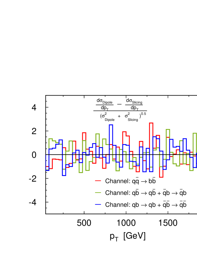
Figure B.1: Difference between results based on dipole formalism and phase space slicing for the differential cross sections for the different quark-induced channels in terms of standard deviations. For the comparison only the relevant IR contributions (boxes and real corrections) were taken into account.

Appendix C Box diagrams for gluon fusion

$$\overline{\sum}\left|{\cal{M}}^{\Box_{Z}\>\>{\alpha_{s}^{2}\alpha}}_{gg\rightarrow b\bar{b}}\right|^{2} = 2\*\pi\*{\alpha_{s}^{2}\alpha}\*{1\over s}\*{2-N^{2}+N^{2}\*z\over N\*(N^{2}-1)}({g_{v}^{b}}^{2}+{g_{a}^{b}}^{2}){1\over 1+z}\*$$ (C.1)

$$\Bigg{\{}4\*(s+{m_{Z}}^{2})+(s+4\*{m_{Z}}^{2})\*z+(5\*s+2\*{m_{Z}}^{2})\*z^{2}$$

$$- (1+z)\*(-2\*s+(3\*s+2\*{m_{Z}}^{2})\*z)\*\ln\left({s\over{m_{Z}}^{2}}\right)$$

$$- {s\*(1+z)+2\*{m_{Z}}^{2}\over s\*(1+z)}\*(6\*s+4\*{m_{Z}}^{2}-(s-2\*{m_{Z}}^{2})\*z+s\*z^{2})\ln\left(1-{t\over{m_{Z}}^{2}}\right)$$

$$- {2\*(s+{m_{Z}}^{2})^{2}\*(1+z)\*(4-z+z^{2})\over s\*(1-z)}$$

$$\times \left[\mbox{Li}_{2}\left(-{s\over{m_{Z}}^{2}}\right)+\ln\left({s\over{m_{Z}}^{2}}\right)\*\ln\left(1+{s\over{m_{Z}}^{2}}\right)\right]$$

$$+ {2\over s\*(1-z)}\*\Big{(}5\*s^{2}+12\*s\*{m_{Z}}^{2}+8\*{m_{Z}}^{4}+2\*s\*(s+2\*{m_{Z}}^{2})\*z+s^{2}\*z^{2}\Big{)}$$

$$\times \left[\mbox{Li}_{2}\left(t\over{m_{Z}}^{2}\right)+\ln\left(s\over{m_{Z}}^{2}\right)\*\ln\left(1-{t\over{m_{Z}}^{2}}\right)\right]\Bigg{\}}+(z\rightarrow-z),$$

$$\overline{\sum}|{{\cal M}}^{\Box_{W}(gg\rightarrow b\bar{b})}|^{2} = 4\*\pi\alpha_{s}^{2}\alpha\*{1\over s}\*{2-N^{2}+N^{2}\*z\over N\*(N^{2}-1)}\*{g_{W}}^{2}\*{1\over 1+z}\*$$ (C.2)

$$\Bigg{\{}s\*z\*(1+z)+{2\over{m_{t}}^{2}-{m_{W}}^{2}}\*\Big{(}2\*(s-{m_{t}}^{2}+{m_{W}}^{2})$$

$$- 2\*({m_{t}}^{2}-{m_{W}}^{2})\*z+(2\*s-{m_{t}}^{2}+{m_{W}}^{2})\*z^{2}\Big{)}\*\Big{(}{\overline{\rm A}_{0}({m_{W}}^{2})}-{\overline{\rm A}_{0}({m_{t}}^{2})}\Big{)}$$

$$- (1+z)\*\Big{(}2\*s-(3\*s-2\*{m_{t}}^{2}+2\*{m_{W}}^{2})\*z\Big{)}\*{\overline{\rm B}_{0}(s,{m_{t}}^{2},{m_{t}}^{2})}$$

$$+ \Big{(}6\*s-4\*{m_{t}}^{2}+4\*{m_{W}}^{2}-(s+2\*mt^{2}-2\*{m_{W}}^{2})\*z+s\*z^{2}\Big{)}\*\overline{\rm B}_{0}(t,{m_{t}}^{2},{m_{W}}^{2})$$

$$- {1\over 1-z}\*\Big{(}5\*s^{2}+4\*s\*(3\*{m_{W}}^{2}-2\*{m_{t}}^{2})+8\*({m_{t}}^{2}-{m_{W}}^{2})^{2}$$

$$+ 2\*s\*(s-2\*{m_{t}}^{2}+2\*{m_{W}}^{2})\*z+s^{2}\*z^{2}\Big{)}$$

$$\times \*\Big{(}{\rm C}_{0}(s,{m_{t}}^{2},{m_{t}}^{2},{m_{t}}^{2})-(1+z)\*{\rm C}_{0}(t,{m_{t}}^{2},{m_{t}}^{2},{m_{W}}^{2})\Big{)}$$

$$- {1\over 1-z}\*\Big{[}s\*(3\*s-4\*{m_{t}}^{2}+4\*{m_{W}}^{2})$$

$$+ \Big{(}2\*s\*(2\*s-3\*{m_{t}}^{2}+4\*{m_{W}}^{2})+6\*({m_{t}}^{2}-{m_{W}}^{2})^{2}\Big{)}\*z$$

$$- s^{2}\*z^{2}+2\*\Big{(}s\*(s-{m_{t}}^{2}+2\*{m_{W}}^{2})+({m_{t}}^{2}-{m_{W}}^{2})^{2}\Big{)}\*z^{3}\Big{]}$$

$$\times {\rm C}_{0}(s,{m_{t}}^{2},{m_{W}}^{2},{m_{t}}^{2})$$

$$- {1\over 2\*(1-z)}\*\Big{[}5\*s^{3}+22\*s^{2}\*{m_{W}}^{2}-10\*s^{2}\*{m_{t}}^{2}$$

$$+ 16\*s\*({m_{t}}^{4}+2\*{m_{W}}^{4}-3\*{m_{t}}^{2}\*{m_{W}}^{2})-16\*({m_{t}}^{2}-{m_{W}}^{2})^{3}$$

$$+ s\*\Big{(}7\*s^{2}-16\*s\*{m_{t}}^{2}+20\*s\*{m_{W}}^{2}+16\*({m_{t}}^{2}-{m_{W}}^{2})^{2}\Big{)}\*z$$

$$+ s\*\Big{(}3\*s^{2}+6\*s\*{m_{W}}^{2}-14\*s\*{m_{t}}^{2}+8\*{m_{t}}^{2}\*({m_{t}}^{2}-{m_{W}}^{2})\Big{)}\*z^{2}+s^{3}\*z^{3}\Big{]}\*{\rm D}_{0}^{W}(z)\Bigg{\}}$$

$$+ (z\rightarrow-z),$$

$$\overline{\sum}|{{\cal M}}^{\Box_{\phi}(gg\rightarrow b\bar{b})}|^{2} = 2\*\pi\*\alpha_{s}^{2}\alpha{1\over s}\*{2-N^{2}+N^{2}\*z\over N\*(N^{2}-1)}\*{g_{W}}^{2}\*{{m_{t}}^{2}\over{m_{W}}^{2}}\*{1\over 1+z}\*$$ (C.3)

$$\Bigg{\{}s\*z\*(1+z)+2\*\Big{(}2\*(1+z)+z^{2}\Big{)}\*\Big{(}{\overline{\rm A}_{0}({m_{t}}^{2})}-{\overline{\rm A}_{0}({m_{W}}^{2})}\Big{)}$$

$$- (1+z)\*\Big{(}2\*s+(s+2\*{m_{t}}^{2}-2\*{m_{W}}^{2})\*z\Big{)}\*{\overline{\rm B}_{0}(s,{m_{t}}^{2},{m_{t}}^{2})}$$

$$+ (2+z)\*\Big{(}s\*(1+z)-2\*({m_{t}}^{2}-{m_{W}}^{2})\Big{)}\*\overline{\rm B}_{0}(t,{m_{t}}^{2},{m_{W}}^{2})$$

$$- {1\over 1-z}\*\Big{(}s^{2}+4\*s\*{m_{W}}^{2}+8\*({m_{t}}^{2}-{m_{W}}^{2})^{2}$$

$$+ 2\*s\*(s-2\*{m_{t}}^{2}+2\*{m_{W}}^{2})\*z+s^{2}\*z^{2}\Big{)}$$

$$\times \*\Big{(}{\rm C}_{0}(s,{m_{t}}^{2},{m_{t}}^{2},{m_{t}}^{2})-(1+z)\*{\rm C}_{0}(t,{m_{t}}^{2},{m_{t}}^{2},{m_{W}}^{2})\Big{)}$$

$$- {1\over 1-z}\*\Big{[}s\*(s-4\*({m_{t}}^{2}-{m_{W}}^{2}))$$

$$+ 2\*\Big{(}s^{2}-s\*{m_{t}}^{2}+2\*s{m_{W}}^{2}+3\*({m_{t}}^{2}-{m_{W}}^{2})^{2}\Big{)}\*z$$

$$+ s^{2}\*z^{2}+2\*(s\*{m_{t}}^{2}+({m_{t}}^{2}-{m_{W}}^{2})^{2})\*z^{3}\Big{]}\*{\rm C}_{0}(s,{m_{t}}^{2},{m_{W}}^{2},{m_{t}}^{2})$$

$$- {1\over 2\*(1-z)}\*\Big{[}s^{3}+6\*s^{2}\*{m_{W}}^{2}-2\*s^{2}\*{m_{t}}^{2}$$

$$+ 16\*s\*{m_{W}}^{2}\*({m_{W}}^{2}-{m_{t}}^{2})+16\*({m_{W}}^{2}-{m_{t}}^{2})^{3}$$

$$+ s\*\Big{(}3\*s^{2}+12\*s\*{m_{W}}^{2}-8\*s\*{m_{t}}^{2}+16\*({m_{t}}^{2}-{m_{W}}^{2})^{2}\Big{)}\*z$$

$$+ s\*\Big{(}3\*s\*(s-2\*{m_{t}}^{2}+2\*{m_{W}}^{2})+8\*{m_{t}}^{2}\*({m_{t}}^{2}-{m_{W}}^{2})\Big{)}\*z^{2}+s^{3}\*z^{3}\Big{]}\*{\rm D}_{0}^{W}(z)\Bigg{\}}$$

$$+ (z\rightarrow-z).$$

References

- [1] P. Nason, S. Dawson and R. K. Ellis, Nucl. Phys. B 327, 49 (1989) [Erratum-ibid. B 335, 260 (1990)].
- [2] W. Beenakker, H. Kuijf, W. L. van Neerven and J. Smith, Phys. Rev. D 40 (1989) 54.
- [3] R. K. Ellis and J. C. Sexton, Nucl. Phys. B 269 (1986) 445.
- [4] W. T. Giele, E. W. N. Glover and D. A. Kosower, Nucl. Phys. B 403, 633 (1993) [arXiv:hep-ph/9302225].
- [5] J. H. Kühn, A. Kulesza, S. Pozzorini and M. Schulze, Nucl. Phys. B 727, 368 (2005) [arXiv:hep-ph/0507178].
- [6] J. H. Kühn, A. Kulesza, S. Pozzorini and M. Schulze, JHEP 0603, 059 (2006) [arXiv:hep-ph/0508253].
- [7] J. H. Kühn, A. Kulesza, S. Pozzorini and M. Schulze, Nucl. Phys. B 797, 27 (2008) [arXiv:0708.0476 [hep-ph]].
- [8] S. Moretti, M. R. Nolten and D. A. Ross, Phys. Lett. B 639, 513 (2006) [Erratum-ibid. B 660, 607 (2008)] [arXiv:hep-ph/0603083].
- [9] S. Moretti, M. R. Nolten and D. A. Ross, Nucl. Phys. B 759, 50 (2006) [arXiv:hep-ph/0606201].
- [10] W. Beenakker, A. Denner, W. Hollik, R. Mertig, T. Sack and D. Wackeroth, Nucl. Phys. B 411 (1994) 343.
- [11] J. H. Kühn, A. Scharf and P. Uwer, Eur. Phys. J. C 45 (2006) 139 [arXiv:hep-ph/0508092].
- [12] J. H. Kühn, A. Scharf and P. Uwer, Eur. Phys. J. C 51 (2007) 37 [arXiv:hep-ph/0610335].
- [13] W. Bernreuther, M. Fuecker and Z. G. Si, Phys. Rev. D 74, 113005 (2006) [arXiv:hep-ph/0610334].
- [14] J. H. Kuhn and A. A. Penin, arXiv:hep-ph/9906545.
- [15] J. H. Kuhn, A. A. Penin and V. A. Smirnov, Eur. Phys. J. C 17, 97 (2000) [arXiv:hep-ph/9912503].
- [16] J. H. Kuhn, S. Moch, A. A. Penin and V. A. Smirnov, Nucl. Phys. B 616, 286 (2001) [Erratum-ibid. B 648, 455 (2003)] [arXiv:hep-ph/0106298].
- [17] B. Feucht, J. H. Kuhn, A. A. Penin and V. A. Smirnov, Phys. Rev. Lett. 93, 101802 (2004) [arXiv:hep-ph/0404082].
- [18] B. Jantzen, J. H. Kuhn, A. A. Penin and V. A. Smirnov, Nucl. Phys. B 731, 188 (2005) [Erratum-ibid. B 752, 327 (2006)] [arXiv:hep-ph/0509157].
- [19] M. Beccaria, G. Montagna, F. Piccinini, F. M. Renard and C. Verzegnassi, Phys. Rev. D 58 (1998) 093014 [arXiv:hep-ph/9805250].
- [20] P. Ciafaloni and D. Comelli, Phys. Lett. B 446 (1999) 278 [arXiv:hep-ph/9809321].
- [21] V. S. Fadin, L. N. Lipatov, A. D. Martin and M. Melles, processes,” Phys. Rev. D 61 (2000) 094002 [arXiv:hep-ph/9910338].
- [22] M. Beccaria et al., Phys. Rev. D 61 (2000) 011301; D 61 (2000) 073005.
- [23] A. Denner and S. Pozzorini, Eur. Phys. J. C 18 (2001) 461 [arXiv:hep-ph/0010201]. A. Denner and S. Pozzorini, Eur. Phys. J. C 21 (2001) 63 [arXiv:hep-ph/0104127].
- [24] E. Maina, S. Moretti, M. R. Nolten and D. A. Ross, Phys. Lett. B 570 (2003) 205 [arXiv:hep-ph/0307021].
- [25] G. Passarino and M. J. G. Veltman, Nucl. Phys. B 160 (1979) 151.
- [26] G. J. van Oldenborgh, Comput. Phys. Commun. 66 (1991) 1.
- [27] A. Denner, Fortsch. Phys. 41 (1993) 307 [arXiv:0709.1075 [hep-ph]].
- [28] J. H. Kuhn and R. G. Stuart, Phys. Lett. B 200, 360 (1988).
- [29] S. Jadach, J. H. Kuhn, R. G. Stuart and Z. Was, Z. Phys. C 38, 609 (1988) [Erratum-ibid. C 45, 528 (1990)].
- [30] S. Catani and M. H. Seymour, Nucl. Phys. B 485 (1997) 291 [Erratum-ibid. B 510 (1998) 503] [arXiv:hep-ph/9605323].