Magellan Spectroscopy of Low-Redshift Active Galactic Nuclei

Abstract

We present an atlas of moderate-resolution ($R\approx 1200-1600$) optical spectra of 94 low-redshift ($z$ $\mathrel{\hbox{\hbox to0.0pt{\hbox{\lower 4.0pt\hbox{$\sim$}}\hss}\hbox{$<$}}}$ 0.5) active galactic nuclei taken with the Magellan 6.5 m Clay Telescope. The spectra mostly cover the rest-frame region $\sim 3600-6000$ Å. All the objects have preexisting Hubble Space Telescope imaging, and they were chosen as part of an ongoing program to investigate the relationship between black hole mass and their host galaxy properties. A significant fraction of the sample has no previous quantitative spectroscopic measurements in the literature. We perform spectral decomposition of the spectra and present detailed fits and basic measurements of several commonly used broad and narrow emission lines, including [O II] $\lambda$3727, He II $\lambda$4686, H$\beta$, and [O III] $\lambda$$\lambda$4959, 5007. Eight of the objects are narrow-line sources that were previously misclassified as broad-line (type 1) Seyfert galaxies; of these, five appear not to be accretion-powered.

1 Introduction

The spectral properties of active galactic nuclei (AGNs) are pertinent to many areas of astrophysics. With the recent interest in massive black holes and their apparently close connection with galaxy evolution (see Ho 2004, and references therein), there has been a resurgence of attention on AGN properties that might lead to expedient methods to estimate black hole masses for large samples of objects. A very promising technique exploits the velocity width of the broad emission lines in type 1 sources, in combination with the size of the line-emitting region estimated from the luminosity of the central source (Kaspi et al. 2005; Bentz et al. 2009), to calculate the “virial mass” of the black hole. This technique has been calibrated for local AGNs using the H$\beta$ (Kaspi et al. 2000) and H$\alpha$ (Greene & Ho 2005b) lines, and for higher redshift sources using ultraviolet lines (C IV $\lambda$1549: Vestergaard 2002; Mg II $\lambda$2800: McLure & Jarvis 2002). At the same time, the characteristics of the narrow emission lines themselves provide useful clues on the impact of AGN activity on certain aspects of the host galaxy (e.g., Netzer et al. 2004; Ho 2005; Kim et al. 2006).

This paper presents an atlas of moderate-resolution optical spectra of 94 low-redshift ($z$ $\mathrel{\hbox{\hbox to0.0pt{\hbox{\lower 4.0pt\hbox{$\sim$}}\hss}\hbox{$<$}}}$ 0.5), mostly broad-line (type 1) AGNs. The spectra have relatively high signal-to-noise ratios (S/N) and moderate resolution ($R=\lambda/\Delta\lambda\approx 1200-1600$), covering predominantly the rest-frame region $\sim 3600-6000$ Å. The observations were taken as part of an ongoing program to investigate the relationship between active black holes and their host galaxies. The ground-based, optical spectra provide the necessary material to estimate black hole masses, and existing images in the Hubble Space Telescope (HST) data archives give details on the host galaxy morphologies and structural parameters (for initial results, see Kim et al. 2007, 2008). Although many of the AGNs are bright, well-known sources, most of them do not have reliable, modern spectra. Of those that do, the published spectra often have highly heterogeneous quality or were analyzed in a manner inadequate for our purposes. The majority of the sample, in fact, was chosen to overlap with the AGNs selected from the Einstein Observatory Extended Medium-Sensitivity Survey (EMSS; Gioia et al. 1990), an unbiased subset of which was uniformly surveyed with HST by Schade et al. (2000). Schade et al. objects constitute an important component of our ongoing host galaxy investigations. The original optical classifications of the EMSS AGNs were based on the spectroscopy of Stocke et al. (1991), but these authors did not publish the actual spectra, nor did they present quantitative analysis of them. We have therefore decided to reobserve as many of the objects as possible from the list of Schade et al. (2000); of the 76 objects in their sample, we observed 61 (80%). When time permitted, we also observed additional targets from the HST studies of low-redshift quasars by Hamilton et al. (2002) and Dunlop et al. (2003) because we also draw heavily on these samples. Some of these brighter objects already have good-quality spectra in the literature (e.g., Boroson & Green 1992; Marziani et al. 2003), but we reobserved them anyway for the sake of homogeneity.

This paper is organized as follows. Section 2 describes the observations and data reductions. Section 3 presents our method of spectral decomposition and the resulting measurements. The spectral atlas is shown in Section 4. Section 5 provides a brief summary. Distance-dependent quantities are calculated assuming the following cosmological parameters: $H_{0}=71$ km s^-1 Mpc^-1, $\Omega_{m}=0.27$, and $\Omega_{\Lambda}=0.75$ (Spergel et al.  2003).

2 Observations and Data Reductions

The observations were obtained with the Magellan 6.5 m Clay Telescope on three observing runs in 23–28 February 2004, 14–18 September 2004, and 7–10 March 2005. Table 1 gives a log of the observations. The data were acquired as part of a backup program for a project that required exceptionally good seeing. We turned to the AGNs whenever the seeing conditions deteriorated to $\mathrel{\hbox{\hbox to0.0pt{\hbox{\lower 4.0pt\hbox{$\sim$}}\hss}\hbox{$>$}}}$ 1^′′, which is considered relatively poor by the standards of Las Campanas Observatory.

During the two 2004 observing runs, we used the now-retired Boller & Chivens (B&C) long-slit (length 2^′) spectrograph equipped with a 2048$\times$515 Marconi chip. The 13.5 $\mu$m pixels project to a scale of 0$\farcs$25. With a slit width of 0$\farcs$75, the

600 lines mm^-1 grating gave an average full-width at half maximum (FWHM) resolution of 4.2 Å (250 km s^-1 at 5000 Å). The spectral resolution, as judged by the widths of the comparison arc-lamp spectra and the night sky lines, was relatively uniform across the spectrum. Two grating tilts were used in order to observe the rest-frame region of most interest to us, 4200–5750 Å, which contains the diagnostically important lines of He II $\lambda$4686, H$\beta$, [O III] $\lambda$$\lambda$4959, 5007, and two of the prominent optical Fe II blends. For sources with $z\leq 0.185$, we covered the spectral range $\sim 3640-6820$ Å; for those with $z>0.185$, the grating tilt was set to cover $\sim 4900-8075$ Å.

The 2005 run employed the Low-Dispersion Survey Spectrograph (LDSS3) in long-slit mode. The 4096$\times$4096 detector has 15 $\mu$m pixels and a scale of 0$\farcs$189 pixel^-1. We cut three slit masks, each with a long slit 0$\farcs$8 wide, which, in combination with a blue and a red volume-phase holographic grating, gave us a total of four spectral settings, each covering $\sim 2500$ Å. The 1090 lines mm^-1 blue grating has a spectral resolution of FWHM = 3.2 Å (190 km s^-1 at 5000 Å), and the 660 lines mm^-1 red grating has a spectral resolution of FWHM = 6.5 Å (245 km s^-1 at 8000 Å).

Pixel-to-pixel variations in the response of the CCD were corrected using domeflats illuminated by external quartz lamps. The B&C data show low-level fringing at wavelengths longer than $\sim 6000$ Å. To remove this effect, for each science image we generated a hybrid flat by combining a contemporaneous domeflat for $\lambda>6000$ Å with a high-S/N flat for shorter wavelengths derived from median-combining a large number (40) of afternoon domeflats. Bias correction was achieved by subtracting a constant count level determined from the overscan region of the chip. We took dark frames to verify that the CCDs indeed have sufficiently low dark current that it can be ignored. The spectra were wavelength-calibrated using comparison arc-lamp spectra, taken at the position of each target, of He+Ar for the B&C runs and He+Ar+Ne for the LDSS3 run. The wavelength solution is typically accurate to $\sim 0.03$ Å rms.

We observed a number of bright G and K giant and subgiant stars, as well as a few A-type dwarfs, to model the host galaxy starlight (Section 3). To perform relative flux calibration, we observed spectrophotometric standard stars with nearly featureless continua—usually white dwarfs (Stone & Baldwin 1983; Baldwin & Stone 1984)—at two widely separated airmasses at the beginning and end of each night. Because of the narrowness of the slit and the (deliberately) non-optimal conditions of the observations, the absolute flux scale is not accurate. To obtain an approximate absolute flux calibration, we empirically bootstrap the observed flux scale to flux densities estimated from optical magnitudes collected from the literature (Table 1). Whenever possible, we chose literature fluxes that were taken with the smallest possible aperture in order to mimic our narrow slit width. As the literature values are quite heterogeneous, our final fluxes are only approximate, accurate perhaps to no better than a factor of $\sim 2$.

Most of the observations were taken with the slit oriented at the parallactic angle to minimize slit losses from atmospheric differential refraction (Filippenko 1982). In a few cases where this was not true, and the airmass was substantial, slit losses introduced significant distortion of the continuum shape in the blue. The total exposure time of each target varied from 90 to 3600 s, depending on the apparent brightness of the source and the prevailing weather conditions (some objects were observed under heavy cloud cover). To the extent possible, we attempted to reach a uniform minimum S/N threshold ($\sim 50-60$ per pixel in the continuum), as judged from real-time, quick-look reduction of the data. This was not always realized because of the challenging sky conditions. Multiple (long $+$ short) exposures were taken of some objects to prevent saturation of the brightest emission lines.

We reduced the spectra following standard procedures within the IRAF package longslit. Prior to generating one-dimensional spectra, which uses optimal extraction (Horne 1986), we removed cosmic rays using the algorithm of van Dokkum (2001). Sky subtraction for the B&C data was performed in a straightforward manner by averaging background regions on either side of the object. However, the LDSS3 data required more extensive treatment, incorporated into the COSMOS data reduction package, in order to rectify the significant curvature in the spatial direction of the images. In the end, the sky subtraction for the LDSS3 data was not fully satisfactory, and regions of the spectra near strong night sky lines were adversely affected. In most instances, this has no significant scientific impact, but in a few objects important spectral features were partly corrupted. For cosmetic purposes, in the final presentation of the spectra, we removed the small affected regions by interpolation. Finally, regions of the spectrum in long exposures that were saturated were replaced with suitably scaled portions from the shorter, unsaturated exposure.

Telluric oxygen absorption lines near 6280 Å, 6860 Å (the “B band”), and 7580 Å (the “A band”) were removed by division of normalized, intrinsically featureless spectra of the standard stars. Large residuals caused by mismatches at the strong bandheads were eliminated by interpolation in the plotted spectra. The reduction procedure also corrected for continuum atmospheric extinction.

3 Spectral Atlas

Figure 1 presents the spectra for the sources, arranged in increasing alphanumeric order. Each panel shows the final spectrum, corrected for foreground Galactic extinction using the $B$-band extinctions given by Schlegel et al. (1998) and the extinction curve of Cardelli et al. (1989). We shifted the spectra to the source rest-frame using the heliocentric radial velocity determined from the centroid of the narrow core of the [O III] $\lambda$5007 line (see Section 4), as listed in Table 1. The [O III] centroid is typically accurate to $\sim$0.13 Å, or $\sim$7.8 km s^-1, consistent with independent checks from published redshifts given in the NASA/IPAC Extragalactic Database (NED). For the purposes of the presentation, a few objects [whose names are followed by “(s)”] with particularly low S/N have been smoothed with a 5-pixel boxcar. As explained in Section 2, the flux density scale is only approximate; the reader should exercise caution in using it for quantitative analysis. These spectra are available upon request from the authors.

Figure 1: Spectral atlas. The ordinate is in units of $10^{-16}$ erg s^-1 cm^-2 Å^-1. Objects marked with “(s)” were smoothed with a 5-pixel boxcar.

Figure 1: Spectral atlas. The ordinate is in units of $10^{-16}$ erg s^-1 cm^-2 Å^-1. Objects marked with “(s)” were smoothed with a 5-pixel boxcar.

Figure 1: Spectral atlas. The ordinate is in units of $10^{-16}$ erg s^-1 cm^-2 Å^-1. Objects marked with “(s)” were smoothed with a 5-pixel boxcar.

Figure 1: Spectral atlas. The ordinate is in units of $10^{-16}$ erg s^-1 cm^-2 Å^-1. Objects marked with “(s)” were smoothed with a 5-pixel boxcar.

Figure 1: Spectral atlas. The ordinate is in units of $10^{-16}$ erg s^-1 cm^-2 Å^-1. Objects marked with “(s)” were smoothed with a 5-pixel boxcar.

Figure 1: Spectral atlas. The ordinate is in units of $10^{-16}$ erg s^-1 cm^-2 Å^-1. Objects marked with “(s)” were smoothed with a 5-pixel boxcar.

Figure 1: Spectral atlas. The ordinate is in units of $10^{-16}$ erg s^-1 cm^-2 Å^-1. Objects marked with “(s)” were smoothed with a 5-pixel boxcar.

Figure 1: Spectral atlas. The ordinate is in units of $10^{-16}$ erg s^-1 cm^-2 Å^-1. Objects marked with “(s)” were smoothed with a 5-pixel boxcar.

Figure 1: Spectral atlas. The ordinate is in units of $10^{-16}$ erg s^-1 cm^-2 Å^-1. Objects marked with “(s)” were smoothed with a 5-pixel boxcar.

Figure 1: Spectral atlas. The ordinate is in units of $10^{-16}$ erg s^-1 cm^-2 Å^-1. Objects marked with “(s)” were smoothed with a 5-pixel boxcar.

Figure 1: Spectral atlas. The ordinate is in units of $10^{-16}$ erg s^-1 cm^-2 Å^-1. Objects marked with “(s)” were smoothed with a 5-pixel boxcar.

Figure 1: Spectral atlas. The ordinate is in units of $10^{-16}$ erg s^-1 cm^-2 Å^-1. Objects marked with “(s)” were smoothed with a 5-pixel boxcar.

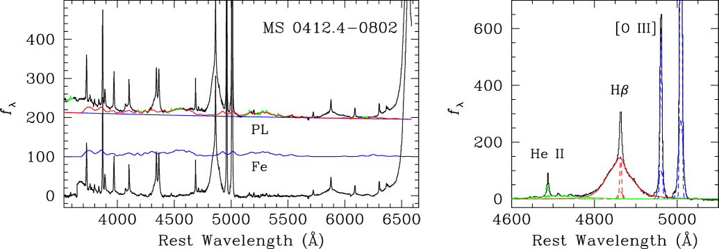
Figure 2: Example of spectral decomposition for MS 0412.4$-$0802. The ordinate is in units of $10^{-17}$ erg s^-1 cm^-2 Å^-1. The left panel shows the original data (black histograms), the different components of the continuum fit (blue lines; “PL” = power law, “Fe” = iron template), and the final model (red line), each offset in the ordinate by a constant, arbitrary amount for clarity. The regions used in the fit are highlighted in green. The bottom plot shows the residual, pure emission-line spectrum. The right panel illustrates our procedure for line fitting for He II (green), H$\beta$ (red), and [O  III] $\lambda$$\lambda$4959, 5007 (blue); solid and dashed lines denote broad and narrow components, respectively.

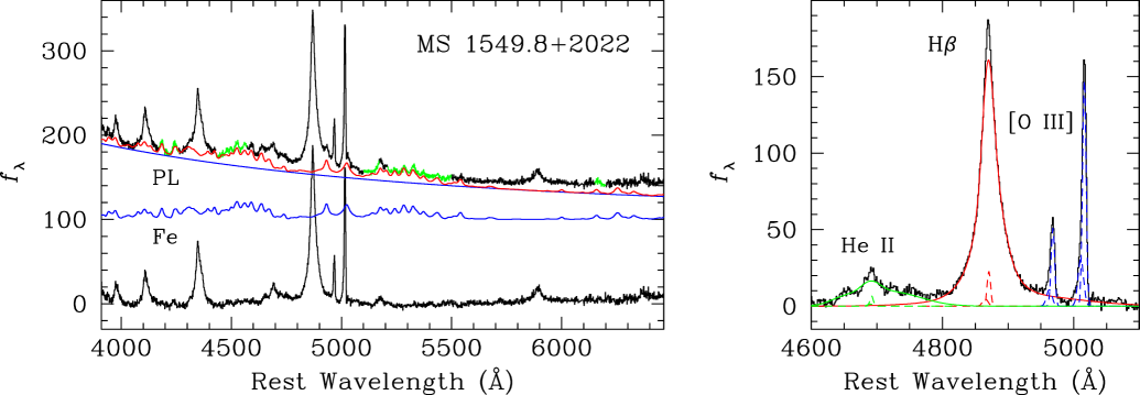
Figure 3: Example of spectral decomposition for MS 1549.8$+$2022; conventions same as in Figure 2.

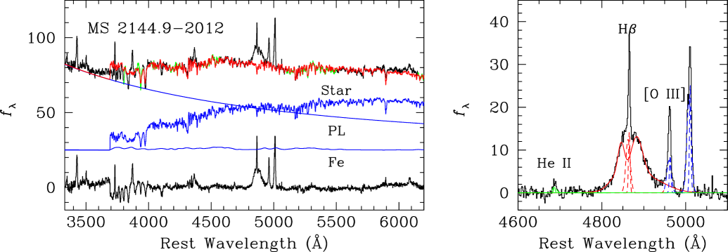
Figure 4: Example of spectral decomposition for MS 2144.9$-$2012; conventions same as in Figure 2, except that the continuum model in this case contains a component for starlight (“Star”) from the host galaxy.

4 Measurements

4.1 Spectral Decomposition

Although the primary purpose of this paper is to present the spectral atlas of our database, we also measure a number of basic spectral parameters for the continuum and strong emission lines commonly used by the AGN community. Our own forthcoming host galaxy analyses will draw heavily from this database. These measurements are summarized in Table 2. Because of our wavelength coverage, we concentrate on the following emission lines: [O II] $\lambda$3727, Fe II $\lambda$4570, He II $\lambda$4686, H$\beta$ $\lambda$4861, and [O III] $\lambda$$\lambda$4959, 5007. Our approach closely follows that of Greene & Ho (2005b) and Kim et al. (2006), which the reader can consult for more details. Here we briefly summarize a few key points.

The optical continuum is a complex mixture of several components, which must be modeled and subtracted prior to measuring the emission lines. We decompose the continuum using a model consisting of up to three components: (1) starlight from the host galaxy, (2) featureless continuum from the AGN, and (3) Fe II emission. We do not account for internal extinction, as there is no unambiguous, universally accepted method of doing so this type of data. We include a galaxy component only if the observed spectrum contains a sufficiently strong starlight component. Following Kim et al. (2006), we require that the equivalent width of the Ca II K line exceed 1.5 Å; this corresponds roughly to a starlight contribution of $\mathrel{\hbox{\hbox to0.0pt{\hbox{\lower 4.0pt\hbox{$\sim$}}\hss}\hbox{$>$}}}$10% to the local continuum. The galaxy continuum is modeled by a linear combination of a G-type and a K-type giant, which, in most cases, suffices to match host galaxies with a predominantly evolved stellar population. Some sources show a significant contribution from intermediate-age stars, as evidenced by the presence of strong higher-order Balmer lines (e.g., MS 1220.9$+$1601, MS 2144.9$-$2012, and MS 2159.5$-$5713; see Figure 1). For these cases adding an additional A-type star does an adequate job of representing the young population. Over the limited wavelength range under consideration, the featureless nonstellar continuum can be approximated using a single power-law function. In a few cases the AGN continuum is slightly more complex, and a better fit can be achieved using the sum of two power-law functions. Finally, blends of broad Fe II transitions form a complicated pseudocontinuum that affects significant portions of the ultraviolet and optical spectrum of most type 1 AGNs. Following standard practice, we model the Fe II component using a scaled and broadened Fe template derived from observations of the narrow-line Seyfert 1 (NLS1) galaxy I Zw 1 (Boroson & Green 1992); the Fe template was kindly provided by T. Boroson. As in Hu et al. (2008a, 2008b), we allow both the width and the radial velocity of the Fe template to be free parameters in the fit, because the kinematics of Fe II need not be identical to those of broad H$\beta$. The Boroson & Green Fe template, unfortunately, does not extend below 3700 Å. Because of this, we do not bother to include the Balmer continuum in the continuum model, since the fit below 3700 Å should not be trusted anyway.

The fit is performed over the following spectral regions devoid of strong emission lines: $3900-3950$, $4020-4070$, $4170-4260$, $4430-4570$, $5100-5170$, $5210-5500$, and $6150-6200$ Å. In practice, however, we adjust the exact fitting regions to achieve the best fit. Figures 2 and 3 give examples of two sources for which the AGN is sufficiently strong that the continuum can be modeled with just the power-law and Fe components; in the case shown in Figure 4, the stellar component clearly must be included too.

After continuum subtraction, we fit the residual spectrum in order to measure the parameters of several prominent emission lines. For the narrow emission lines, we follow the same procedure used by Kim et al. (2006). If the [S II] $\lambda$$\lambda$6716, 6731 doublet is included in the bandpass and the S/N is adequate, we use the profile of [S II] to constraint [N II] $\lambda$$\lambda$6548, 6583 and the the narrow component of H$\alpha$ and H$\beta$. However, in the majority of the objects [S II] lies outside of our spectral coverage. In this situation we have no choice but to rely on [O III] as a template for the narrow lines. As in Greene & Ho (2005a), we fit each of the lines of the [O III] $\lambda$$\lambda$4959, 5007 doublet with one or two Gaussians, depending on whether they show an extended or asymmetric wing. With the profile of the narrow component thus constrained, we fit the broad component of the permitted lines using as many Gaussian components as necessary to achieve an acceptable fit (typically only 2–3 suffice).

The He II $\lambda$4686 emission line, while diagnostically important, is challenging to measure accurately because it is much weaker than H$\beta$ and because it lies on the shoulder of the strong Fe II $\lambda$4570 blend to the blue and H$\beta$ to the red. We treat He II in the same manner as H$\beta$, using [O III] as a template for its narrow component, and a multi-Gaussian model for the broad component. If either component is undetected, we set an upper limit based on 3 times the rms noise of the local continuum and an assumed velocity width; for the narrow component, we use the [O III] profile, whereas the broad H$\beta$ profile is used for the broad component.

As in previous studies (e.g., Boroson & Green 1992; Marziani et al. 2003), we select the prominent Fe II blend at 4570 Å to represent the strength of the optical Fe emission. The flux of the feature is integrated over the region 4434–4684 Å. If undetected, we calculate the 3 $\sigma$ upper limit from the rms noise over this region.

Finally, we give measurements for [O II] $\lambda$3727, whose strength provides constraints on the ongoing star formation rate in AGNs (Ho 2005). As in Kim et al. (2006; see also Kuraszkiewicz et al. 2000), we measure the line strength by simply fitting a single Gaussian with respect to the local continuum near 3700 Å. This procedure suffices because the [O II] doublet remains unresolved at the relatively low resolution of our observations, and measuring the line locally bypasses the complications of the poor continuum fits in the blue part of the spectra. Upper limits are set using the local rms noise and the velocity width of [O III].

The velocity widths of [O III] listed in Table 2 pertain to the FWHM of the final model for the entire line profile, and have been corrected for instrumental resolution by subtracting it in quadrature.

4.2 Uncertainties

Robust uncertainties are notoriously difficult to derive for spectral measurements of the type presented above. In almost all cases the formal error bars from the fits underestimate the true errors, which are dominated by systematic uncertainties in the myriad assumptions that enter into the complicated fits. For this reason we resist assigning specific error bars to the entries in Table 2. Nevertheless, based on past experience with analysis of this type (e.g., Ho et al. 1997; Greene & Ho 2005b; Kim et al. 2006; Hu et al. 2008a, 2008b), in the notes to Table 2 we give some rough estimates of the typical uncertainties involved.

5 General Properties of the EMSS AGNs

As the EMSS AGNs have never been analyzed spectroscopically in a quantitative manner, and our survey contains a significant fraction (80%) of the sample studied by Schade et al. (2000), we will give a few general statistics on the spectroscopic properties of these objects. The EMSS was conducted in the 0.3–3.5 keV band and, as such, is expected to be biased toward sources that are bright in soft X-rays. Because of their strong soft X-ray emission (e.g., Boller et al. 1996; Grupe et al. 2004), NLS1s should be overrepresented in AGNs selected on the basis of their soft X-ray emission compared to selection in other wavelengths (e.g., optical). This is especially true because of the relatively low luminosities probed by the EMSS. We confirm this expectation. Among the 51 EMSS sources with detected broad H$\beta$ emission, 33% have H$\beta$ FWHM $<$ 2000 km s^-1, the conventional linewidth criterion for NLS1s. This fraction increases to 47% if we relax the (somewhat arbitrary) FWHM cutoff to 2500 km s^-1. As expected from previous studies, these sources tend to show relatively weak [O III] lines but prominent Fe II emission. By comparison, within the sample of $\sim 8500$ low-redshift ($z$ $\mathrel{\hbox{\hbox to0.0pt{\hbox{\lower 4.0pt\hbox{$\sim$}}\hss}\hbox{$<$}}}$0.35), optically selected type 1 AGNs studied by Greene & Ho (2007), the fraction of sources with H$\alpha$ FWHM $<$ 2000 km s^-1 is 24%, increasing to 40% for FWHM $<$ 2500 km s^-1. [To zeroth order, broad H$\alpha$ and H$\beta$ have similar line profiles (Greene & Ho 2005b).]

In terms of their luminosities, all of the EMSS sources should be regarded as Seyferts rather than quasars. Their broad H$\beta$ luminosities range from $\sim 10^{39}$ to $10^{43}$ erg s^-1, with a median value of $\sim 10^{42}$ erg s^-1; using a standard conversion from line to continuum luminosity (Greene & Ho 2005b), this corresponds to a median absolute magnitude of only $M_{B}\approx-19$, roughly near the knee of the luminosity function of local Seyfert galaxies (see Figure 8 in Ho 2008). Despite their modest luminosities, as discussed in M. Kim et al. (in preparation), the EMSS sources are radiating at a healthy fraction of their Eddington rates ($L_{\rm bol}/L_{\rm Edd}\approx 0.01-1$) because their black hole masses are relatively low ($M_{\rm BH}\approx 10^{6}-10^{8}$ $M_{\odot}$), consistent with their hosts being mostly spiral galaxies (Schade et al. 2000).

While our original intent was to observe type 1 AGNs for which we can estimate black hole masses, 10 objects from the EMSS sample turn out to reveal only narrow emission lines in our spectral range (see Table 2). Of these, two have Sloan Digital Sky Survey spectra that extend further to the red than our spectra. MS 1058.8$+$1003 shows a double-peaked broad H$\alpha$ line, and the relative intensities of its narrow lines qualify it as a low-ionization nuclear emission-line region; following the nomenclature of Ho et al. (1997), it should be classified as a LINER 1.9. MS 1414.9$+$1337 also has weak broad H$\alpha$ emission, but its higher-ionization narrow-line spectrum qualifies it as a Seyfert 1.9. As for the rest, only three (MS 0039.0$-$0145, 0516.6$-$4609, and 1110.3$+$2210) appear to be genuine type 2 Seyferts, as judged by their large [O III]/H$\beta$ ratios and, for the latter two, detection of relatively strong [O I] $\lambda$6300. Without the help of the diagnostic lines near H$\alpha$ (see Ho 2008), the physical nature of the remaining five objects — MS 0944.1$+$1333, 1108.3$+$3530, 1114.4$+$1801, 1200.1$-$0330, and 1242.2$+$1632 — is somewhat ambiguous. But judging from the relative strengths of [O II], [O III], and H$\beta$, we suspect that these sources are not powered by AGNs but rather by star formation.

6 Summary

We have used the Magellan 6.5 m Clay Telescope to obtain moderate-resolution ($R\approx 1200-1600$) optical spectra covering the rest-frame region $\sim 3600-6000$ Å for a sample of 94 low-redshift ($z$ $\mathrel{\hbox{\hbox to0.0pt{\hbox{\lower 4.0pt\hbox{$\sim$}}\hss}\hbox{$<$}}}$ 0.5) type 1 AGNs. Although some of the objects are well-known sources, the majority do not have reliable spectroscopy in the literature that can be used to estimate black hole masses from their broad emission lines. We pay special attention to the sample of soft X-ray-selected (EMSS) AGNs with good-quality HST images studied by Schade et al. (2000). Eight of the sources turn out to be narrow-line objects that were previously misclassified as broad-line AGNs; of these only three are Seyfert 2 galaxies and the rest appear to be powered by stars. We present a spectral atlas of our sample and basic measurements for a number of prominent, commonly used emission lines. These data will be used in a separate paper aimed at studying the relationship between black hole mass and the properties of their host galaxies.

References

- (1) Baldwin, J. A., & Stone, R. P. S. 1984, MNRAS, 206, 241
- (2) Bentz, M. C., Peterson, B. M., Netzer, H., Pogge, R. W., & Vestergaard, M. 2009, ApJ, 697, 160
- (3) Boller, T., Brandt, W. N., & Fink, H. 1996, A&A, 305, 53
- (4) Boroson, T. A., & Green, R. F. 1992, ApJS, 80, 109
- (5) Cardelli, J. A., Clayton, G. C., & Mathis, J. S. 1989, ApJ, 345, 245
- (6) Dunlop, J. S., McLure, R. J., Kukula, M. J., Baum, S. A., O’Dea, C. P., & Hughes, D. H. 2003, MNRAS, 340, 1095
- (7) Gioia, I. M., Maccacaro, T., Schild, R. E., Wolter, A., Stocke, J. T., Morris, S. L., & Henry, J. P. 1990, ApJS, 72, 567
- (8) Greene, J. E., & Ho, L. C. 2005a, ApJ, 627, 721
- (9) Greene, J. E., & Ho, L. C. 2005b, ApJ, 630, 122
- (10) Greene, J. E., & Ho, L. C. 2007, ApJ, 667, 131
- (11) Grupe, D., Wills, B. J., Leighly, K. M., & Meusinger, H. 2004, AJ, 127, 156
- (12) Hamilton, T. S., Casertano, S., & Turnshek, D. A. 2002, ApJ, 576, 61
- (13) Ho, L. C. 2004, ed., Carnegie Observatories Astrophysics Series, Vol. 1: Coevolution of Black Holes and Galaxies (Cambridge: Cambridge Univ. Press)
- (14) Ho, L. C. 2005, ApJ, 629, 680
- (15) Ho, L. C. 2008, ARA&A, 46, 475
- (16) Ho, L. C., Filippenko, A. V., & Sargent, W. L. W. 1997, ApJS, 112, 315
- (17) Horne, K. 1986, PASP, 98, 609
- (18) Hu, C., Wang, J.-M., Ho, L. C., Chen, Y.-M., Bian, W.-H., & Xue, S.-J. 2008a, ApJ, 683, L115
- (19) Hu, C., Wang, J.-M., Ho, L. C., Chen, Y.-M., Zhang, H.-T., Bian, W.-H., & Xue, S.-J. 2008b, ApJ, 687, 78
- (20) Kaspi, S., Maoz, D., Netzer, H., Peterson, B. M., Vestergaard, M., & Jannuzi, B. T. 2005, ApJ, 629, 61
- (21) Kaspi, S., Smith, P. S., Netzer, H., Maoz, D., Jannuzi, B. T., & Giveon, U. 2000, ApJ, 533, 631
- (22) Kim, M., Ho, L. C., & Im, M. 2006, ApJ, 642, 702
- (23) Kim, M., Ho, L. C., Peng, C. Y., Barth, A. J., Im, M., Martini, P., & Nelson, C. H. 2008, ApJ, 687, 767
- (24) Kim, M., Ho, L. C., Peng, C. Y., & Im, M. 2007, ApJ, 658, 107
- (25) Kuraszkiewicz, J., Wilkes, B., Brandt, W. N., & Vestergaard, M. 2000, ApJ, 542, 631
- (26) Marziani, P., Sulentic, J. W., Zamorani, R., Calvani, M., Dultzin-Hacyan, D., Bachev, R., & Zwitter, T. 2003, ApJS, 145, 199
- (27) McLure, R. J., & Jarvis, M. J. 2002, MNRAS, 337, 109
- (28) Netzer, H., Shemmer, O., Maiolino, R., Oliva, E., Croom, S., Corbett, E., & di Fabrizio, L. 2004, ApJ, 614, 558
- (29) Schade, D. J., Boyle, B. J., & Letawsky, M. 2000, MNRAS, 315, 498
- (30) Schlegel, D. J., Finkbeiner, D. P., & Davis, M. 1998, ApJ, 500, 525
- (31) Spergel, D. N., et al. 2003, ApJS, 148, 175
- (32) Stocke, J. T., Morris, S. L., Gioia, I. M., Maccacaro, T., Schild, R., Wolter, A., Fleming, T., & Henry, J. P. 1991, ApJS, 76, 813
- (33) Stone, R. P. S., & Baldwin, J. A. 1983, MNRAS, 204, 347
- (34) van Dokkum, P. G. 2001, PASP, 113, 1420
- (35) Vestergaard, M. 2002, ApJ, 571, 733