Quantum interference within the complex quantum Hamilton-Jacobi formalism
Abstract
Quantum interference is investigated within the complex quantum Hamilton-Jacobi formalism. As shown in a previous work [Phys. Rev. Lett. 102, 250401 (2009)], complex quantum trajectories display helical wrapping around stagnation tubes and hyperbolic deflection near vortical tubes, these structures being prominent features of quantum caves in space-time Argand plots. Here, we further analyze the divergence and vorticity of the quantum momentum function along streamlines near poles, showing the intricacy of the complex dynamics. Nevertheless, despite this behavior, we show that the appearance of the well-known interference features (on the real axis) can be easily understood in terms of the rotation of the nodal line in the complex plane. This offers a unified description of interference as well as an elegant and practical method to compute the lifetime for interference features, defined in terms of the average wrapping time, i.e., considering such features as a resonant process.
keywords:
Quantum interference , Complex quantum trajectory , Quantum momentum function , Pólya vector field , Quantum cavePACS:
03.65.Nk , 03.65.Ta , 03.65.Ca1 Introduction
Quantum interference is an observable effect arising from the coherent superposition of quantum probability amplitudes. It is involved in a very wide range of important applications, such as superconducting quantum interference devices or SQUIDs [1, 2], coherent control of chemical reactions [3], atomic and molecular interferometry [4, 5, 6, 7], and Talbot/Talbot-Lau interferometry with relatively heavy particles (e.g., Na atoms [8] and Bose-Einstein condensates [9]). Indeed, possibly one of the main practical applications of interference nowadays is in Bose-Einstein condensate (BEC) interferometry [11, 12, 10] due to its potential use in applications, such as sensing, metrology or quantum information processing. Thus, since the first experimental evidence of interference between two freely expanding BECs was observed [13], an increasing amount of work, both theoretical and experimental, can be found in the literature [14, 15, 16, 17, 18, 19, 20]. Basically, in this type of interferometry there are three steps. First, the atomic cloud is cooled in a magnetic trap until condensation takes place; second, the BEC is split coherently by means of radio-frequency [18] or microwave fields [19]; and third, the double-well-like trapping potential is switched off and the two parts of the BEC are allowed to interfere by free expansion (see, for example, Fig. 6 in Ref. [20] as an illustration of a real experimental outcome). Apart from the practical applications mentioned before, interference plays also an important role when dealing with multipartite entangled systems as an indicator of the loss of coherence induced by the interaction between the different subsystems, commonly referred as “Schrödinger cat states” [21]. However, very little attention beyond the implications of the superposition principle has been devoted to understanding quantum interference at a more fundamental level.
Bohmian mechanics provides an alternative interpretation to quantum mechanics [22, 23, 24]. As an analytical approach, this formulation has been used to analyze atom-surface scattering [25, 26, 27], the quantum Talbot effect [28], quantum nonlocality [29] or quantum interference [30]. As a synthetic approach, the quantum trajectory method (QTM) [31] has been developed as a computational implementation to the hydrodynamic formulation of quantum mechanics to generate the wave function by evolving ensembles of quantum trajectories [32]. However, computational difficulties resulting from interference effects are encountered in regions where the wave packet is reflected from the barrier and nodes or quasi-nodes occur. Thus, a bipolar counter-propagating decomposition approach for the total wave function has been developed to overcome numerical instabilities due to interferences [33, 34, 35, 36, 37, 38, 39].
Here, a more detailed analysis of quantum interference within the complex quantum Hamilton-Jacobi formalism [40, 41] is presented. The complex quantum trajectory method has been applied to stationary problems [42, 43, 44, 45, 46, 47, 48] and to one-dimensional and multi-dimensional wave packet scattering problems [49, 50, 51, 52, 53, 54, 55, 56, 57, 58, 59]. The purpose of this work is to investigate how information can be extracted from this complex formulation regarding interference. Recently, quantum interference associated with superpositions of Gaussian wave packets was thoroughly analyzed using both the standard quantum-mechanical and Bohmian approaches in real space [60, 30]. In spite of its simplicity, such superpositions are experimentally realizable in atom interferometry [61, 62, 63, 64, 65], for example. In contrast to conventional quantum mechanics, Bohmian mechanics offers a trajectory-based understanding of quantum interference. The interference of two wave packets in one real coordinate leads to the formation of nodal structure, and the quantum potential near these nodes forces these trajectories to avoid these regions and to exhibit laminar flow in space-time plots [60]. In contrast, within the complex quantum Hamilton-Jacobi formalism, the collinear collision of two Gaussian wave packets demonstrated caustics and vortical dynamics in the complex plane [60, 66]. This complicated trajectory dynamics cannot be found in Bohmian mechanics unless two or more real coordinates are introduced.
When systematically analyzed for local structures of the quantum momentum function (QMF) and the Pólya vector field (PVF) around its characteristic points [67, 68], complex quantum trajectories display helical wrapping around stagnation tubes and hyperbolic deflection around vortical tubes [66]. This intriguing topological structure is formed by these tubes and gives rise to quantum caves in space-time Argand plots. Quantum interference thus leads to the formation of quantum caves and the appearance of the topological structure mentioned before. In contrast with quantum trajectories, Pólya trajectories display hyperbolic deflection around stagnation tubes and helical wrapping around vortical tubes. The QMF divergence and vorticity characterize the turbulent flow of trajectories, determining the so-called wrapping time [66] for an individual trajectory. Moreover, it is shown that both the PVF divergence and vorticity vanish except at poles, thus the PVF describing an incompressible and irrotational flow.
Trajectories launched from different positions wrap around the same stagnation tubes. Hence, the circulation of trajectories can be viewed as a resonance process, from which one can obtain a natural way to define a “lifetime” for the interference. This information could be therefore used with practical purposes to analyze, explain and understand experiments where interference is the main physical process or mechanism, as in those described above in this Section. The rotational dynamics of the nodal line arising from the interference of wave packets in the complex plane thus offers an elegant method to compute the lifetime for the interference features observed on the real axis.
We consider two cases of head-on collision of two Gaussian wave packets, which depend on the relative magnitude between the propagation velocity and the spreading rate of the wave packets [30]. In the case where the relative propagation velocity is larger than the spreading rate of the wave packets, an average wrapping time is calculated to provide a lifetime for the interference features, while the rotational dynamics of the nodal line in the complex plane explains the transient appearance of the interference features observed on the real axis. In the case where the relative propagation velocity is approximately equal to or smaller than the spreading rate of the wave packets, the rapid spreading of the wave packets leads to a distortion of quantum caves. The infinite survival of interference features in this case implies that the wrapping time becomes infinity. However, the rotational dynamics of the nodal line clearly explains the persistent interference features observed on the real axis. In both cases, the interference features are observed on the real axis when the nodal line is near the real axis; therefore, in contrast to conventional quantum mechanics, the rotational dynamics of the nodal line in the complex plane provides a fundamental interpretation of quantum interference.
The organization of this work is as follows. To be self-contained, in Sec. 2 we briefly describe the complex quantum Hamilton-Jacobi formalism as well as the QMF local structures and its associated PVF near characteristic points. In Sec. 3, first we present theoretical analysis of the Gaussian wave-packet head-on collision on the real axis and in the complex plane, and then demonstrate the interpretation of quantum interference with two cases in the framework of the complex quantum trajectory method. Finally, we present a summary and discussion in Sec. 4.
2 Theoretical formulation
2.1 Complex quantum Hamilton-Jacobi formalism
Substituting the complex-valued wave function expressed by into the time-dependent Schrödinger equation, we obtain the quantum Hamilton-Jacobi equation (QHJE) in the complex quantum Hamilton-Jacobi formalism,
| (1) |
where is the complex action and the last term is the complex quantum potential. In real space, the QMF is defined by , which, within the complex quantum Hamilton-Jacobi formalism, is analytically continued to the complex plane by extending the real variable to a complex variable . The same is done with other relevant functions, such as the wave function and the potential energy. Quantum trajectories in complex space are then determined by solving the guidance equation
| (2) |
where time remains real-valued and the (complex) QMF is expressed in terms of the (complex) wave function (through the complex action) as
| (3) |
From this equation, nodes in the wave function correspond to QMF poles. Moreover, those points where the first derivative of the wave function vanishes will correspond to QMF stagnation points.
2.2 Local structures of the quantum momentum function and its Pólya vector field
The dynamics of complex quantum trajectories is guided by the wave function through the QMF. The complex-valued QMF can be regarded as a vector field in the complex plane. The trajectory dynamics is significantly influenced by both the QMF stagnation points and poles. Streamlines near a QMF stagnation point may spiral into or out of it, or they may become circles or straight lines. The QMF near a pole displays East-West and North-South hyperbolic structure [67, 68]. These local structures around these characteristic points have also been observed for the one-dimensional stationary scattering problems including the Eckart and the hyperbolic tangent barriers [47, 48].
The PVF of a complex vector field is defined by its complex conjugate [70, 71, 69]. Thus, the PVF associated with the QMF, , is given by the vector field . This new vector field provides a simple geometrical and physical interpretation for complex circulation integrals
| (4) |
where denotes a simple closed curve in the complex plane, is tangent to and is normal to and pointing outwards. The real part of the integral in Eq. (4) gives the total amount of work done in moving a particle along a closed contour subjected to , while its imaginary part gives the total flux of the vector field across the closed contour [69].
In Bohmian mechanics, quantum vortices form around nodes in two or more real coordinates [72, 73, 74, 75, 76, 77, 78, 79, 80, 26, 81]. Analogously, in the complex plane quantum vortices form around nodes of the wave function, the quantized circulation integral arising from the discontinuity in the real part of the complex action [67, 68]. The PVF of a complex function contains exactly the same information as the complex function itself, but it is introduced to interpret the circulation integral in terms of the work and flux of its PVF along the contour. Moreover, the PVF is the tangent vector field of contours for the complex-extended Born probability density [82, 83]. Streamlines near a PVF stagnation point display rectangular hyperbolic structure, while streamlines near a PVF pole become circles enclosing the pole [67, 68]. Local structures or streamlines for the QMF and its associated PVF are summarized in Table 1.
| Stagnation point | Pole | |
|---|---|---|
| QMF | Spirals, circles, | East-West and North-South |
| or straight lines | opening hyperbolic flow | |
| PVF | Rectangular | Circular flow |
| hyperbolic flow |
2.3 Approximate quantum trajectories around a stagnation point
Since the QMF is generally time-dependent, we can determine approximate complex quantum trajectories around a stagnation point in spacetime. We expand the QMF in a Taylor series around a stagnation point
| (5) |
where has been used and the partial derivatives are evaluated at the stagnation point. Substituting this equation into Eq. (2), we obtain a first-order nonautonomous complex ordinary differential equation for approximate quantum trajectories
| (6) |
where and have been used and the origin has been moved to the stagnation point. General solutions for the nonautonomous linear differential equation are given by [84]
| (7) | |||||
where is the starting point of a local approximate quantum trajectory. If we consider complex quantum streamlines at a specific time , the QMF does not depend on time. Hence, the partial derivative of the QMF with respect to time is equal to zero, . Thus, the general solution in Eq. (7) gives the approximate quantum streamlines near the stagnation point.
2.4 Divergence and vorticity of the quantum momentum field and its Pólya vector field
The QMF first derivative contains the information about the divergence and vorticity of the quantum fluid in the complex plane [66]. This can be shown as follows. The QMF divergence, which describes the local expansion/contraction of the quantum fluid, is given by
| (8) |
Analogously, the vorticity describing the local rotation of the quantum fluid is defined by the QMF curl,
| (9) |
Since the QMF is analytically extended to the complex plane, we use the Cauchy-Riemann equations to write the QMF first derivative as
| (10) |
Thus, the real and imaginary parts of the QMF first derivative determine the divergence and vorticity, respectively. Moreover, the complex quantum potential in Eq. (1) can be expressed in terms of divergence and vorticity by [66]
| (11) |
Additionally, we can also evaluate both the PVF divergence and vorticity, which are given by
| (12) | ||||
| (13) |
respectively, where the Cauchy-Riemann equations for the QMF have been used. The vanishing divergence and vorticity indicate that the PVF associated with the QMF describes an incompressible and irrotational flow in the complex plane except at nodes of the wave function. Actually, this result follows from the fact that the PVF of a complex function is divergence-free and curl-free if is analytic, and vice versa [69].
The quantized circulation integral around quantum vortices originates from the work term of the PVF in Eq. (4) [67],
| (14) |
The PVF near a pole is expressed in terms of polar coordinates by , where is the circulation and is the radial distance from the center of the vortex. From Eq. (13), the PVF vorticity is zero everywhere except at poles. The PVF velocity near a pole varies inversely as the distance from the core of the vortex. The circulation integral along a closed path enclosing the vortex is equal to , which is independent of . Although the quantum fluid described by the streamlines around a pole moves along a circular path, its vorticity is zero. These features indicate that the quantum vortex described by the PVF is a free or irrotational vortex [85].
2.5 Divergence and vorticity around a pole
For a wave function with an -th order node at , , we can evaluate the QMF first derivative, which yields
| (15) |
where is the smooth part of the QMF. Thus, the QMF first derivative can be approximated by the first term in the vicinity of a pole. For simplicity, we move the origin to the pole. Separating the first term in Eq. (15) into its real and imaginary parts, we obtain the divergence and vorticity around the pole through Eq. (10),
| (16) | ||||
| (17) |
respectively. These approximate forms describe the local behavior of the divergence and vorticity in the vicinity of the pole.
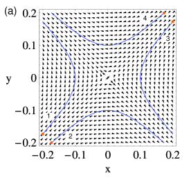
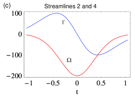
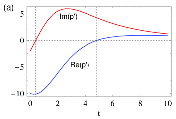
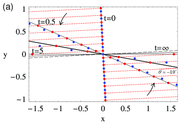
Figure 1 presents the variations of both the QMF divergence and vorticity along the approximate streamlines in the vicinity of a pole. From now on, and atomic units will be used throughout this work. In this case, we consider a wave function with one first-order node at the origin . As discussed in Sec. 2.2, in Fig. 1(a) we observe how the QMF displays a hyperbolic flow around the pole. In addition, streamlines 1 and 3 are parametrized by and streamlines 2 and 4 are parametrized by . In Figs. 1(b) and 1(c), we show the variations of both the QMF divergence and vorticity given by Eqs. (16) and (17), respectively, along the streamlines shown in Fig. 1(a) from to . As can be noticed in these figures, the positive QMF divergence describes the local expansion of the quantum fluid when particles approach the pole. When particles approach turning points near the pole, the QMF divergence vanishes; when particles leave the pole, the negative QMF divergence indicates the local contraction of the quantum fluid. On the other hand, the QMF vorticity describes the local rotation of the quantum fluid. During the whole process, it can be noticed that streamlines 1 and 3 display local counterclockwise rotation, while streamlines 2 and 4 display local clockwise rotation. The QMF vorticity attains the extrema at the turning points. Therefore, when particles approach the pole, they rebound as they experience a repulsive force.

3 Quantum interference
3.1 Head-on collision of two Gaussian wave packets
3.1.1 On the real axis
We consider the Gaussian wave-packet head-on collision which, despite its simplicity, can be considered as representative of other more complicated, realistic processes characterized by interference (e.g., scattering problems, diffraction by slits, etc.). This process can be described by the following total wave function
| (18) |
Each wave packet ( or , left or right, respectively) is represented by a free Gaussian function as
| (19) |
where, for each component, and the complex time-dependent spreading is
| (20) |
with the initial spreading . From Eq. (20), the spreading of this wave packet at time is
| (21) |
Due to the free motion, ( is the propagation velocity) and , i.e., the centroid of the wave packet moves along a classical rectilinear trajectory. This does not mean, however, that the average value of the wave-packet energy is equal to since, due to the quantum potential, the average energy is given by [30]. We observe two contributions in this expression. The former is associated with the translation of the wave packet traveling at velocity , while the latter is related to its spreading at velocity and has, therefore, a purely quantum-mechanical origin. The effective momentum can then be written as , which resembles Heisenberg’s uncertainty relation.
The relationship between and plays an important role in effects that can be observed when dealing with wave packet superpositions [30]. Defining the timescale , we note that, if , the width of the wave packet remains basically constant with time, (i.e., for practical purposes, it is roughly time-independent up to time ). This condition is equivalent to having an initial wave packet prepared with . Thus, the translational motion will be much faster than the spreading of the wave packet. On the contrary, if , which is equivalent to , the width of the wave packet increases linearly with time (), and the wave packet spreads very rapidly in comparison with its advance along . Of course, in between, there is a smooth transition; from Eq. (21), it is shown that the progressive increase of describes a hyperbola when this magnitude is plotted vs time. Thus, we can control in the interference process the spreading and translational motions which determine the wave packet dynamics [60, 30].
3.1.2 In the complex plane
In conventional quantum mechanics, the interference pattern transiently observed on the real axis is attributed to the constructive and destructive interference between two counter-propagating components of the total wave function in Eq. (18). In contrast, in the framework of the complex quantum Hamilton-Jacobi formalism, the total wave function is analytically continued to the complex plane from to . Therefore, two propagating wave packets always interfere with each other in the complex plane, and this leads to a persistent pattern (line) of nodes and stagnation points which rotates counterclockwise with time [60, 66].
The nodal positions in the complex plane can be determined analytically by solving the equation , resulting
| (22) |
where . Here, we have assumed and . Splitting this expression into its real and imaginary parts, i.e., , we obtain
| (23) | ||||
| (24) |
respectively, where is the timescale for the Gaussian wave packet. In addition, dividing Eq. (24) by Eq. (23) yields the analytical expression for the (time-dependent) polar angle describing the angular position of the nodal line with respect to the positive real axis,
| (25) |
which does not depend on . From this expression, we can calculate the rotation rate of the nodal line in the complex plane,
| (26) |
where is given in Eq. (21). This equation indicates that the rotation rate is completely determined by the initial spreading of the Gaussian wave packet . In addition, this rate is always positive and decays monotonically to zero as goes to . From Eqs. (23) and (24), we can also determine the node separation distance between two consecutive nodes
| (27) |
where is the effective momentum. This distance is independent of and it increases with time. Moreover, eliminating in Eqs. (23) and (24) yields the th node trajectory describing the time evolution of the node given by
| (28) |
Consequently, these nodal trajectories with the same slope and different intercepts are parallel to each other.
When , the initial angle of the nodal line is . As described by Eq. (26), the positive rotational rate indicates that the polar angle of the nodal line increases monotonically with time. The nodal line thus rotates counterclockwise from the initial angle to a maximum or limiting value when . The angular displacement from to is always equal to , because the product of the slopes of the nodal lines is equal to . In particular, if both wave packets are initially very far apart (i.e., ), but move with a finite velocity , or they are at an arbitrary finite distance, but , the nodal line ends up aligned with the real axis. Otherwise, the nodal line starts at some angle and then evolves with the angular displacement until it reaches the limit angle . In addition, the initial nodal line is perpendicular to all nodal trajectories in Eq. (28). Then, the nodal line rotates counterclockwise with time and it becomes parallel to nodal trajectories when approaches infinity.
Interference features are observed on the real axis only when the nodal line is near the real axis. When the nodal line coincides with the real axis, the maximum interference features can be observed in real space. At this time, setting in Eq. (28), we recover the expression for the positions of nodes on the real axis, where . During the evolution of the nodal line, its intersections with nodal trajectories determine the positions of the nodes. As can be noticed, the time evolution of the nodal line in the complex plane therefore provides an elegant interpretation of quantum interference.
3.2 Case 1:
We first consider the case where the relative propagation velocity is larger than the spreading rate of the wave packets. The following initial conditions for Gaussian wave packets are used: , and . With these conditions, maximal interference occurs at on the real axis and the propagation and spreading velocities are given by and , respectively.
3.2.1 Quantum caves with quantum trajectories
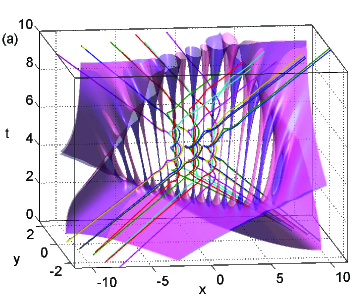
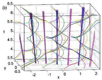
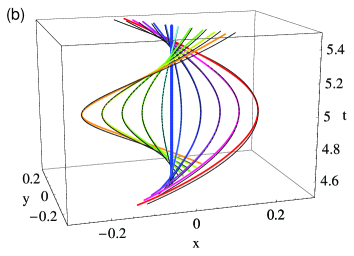
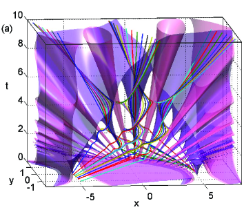
Figure 2(a) displays complex quantum trajectories with the quantum caves consisting of the isosurfaces and from to in a time-dependent three-dimensional Argand plot. As discussed in Sec. 2.2, the QMF local structures near stagnation points and poles provide a qualitative description of the behavior of these trajectories. It is clearly seen that stagnation and vortical tubes alternate with each other, and the centers of the tubes are stagnation and vortical curves. Trajectories display helical wrapping around the stagnation tubes and they are deflected by the vortical tubes to show hyperbolic indentations in three dimensional space, as shown in Fig. 2(b). These trajectories, which display complicated paths around stagnation and vortical tubes, depict how probability flows. In addition, trajectories from different launch points wrap around the same stagnation curve and remain trapped for a certain time interval. Then, they separate from the stagnation curve. This counterclockwise circulation of trajectories can be viewed as a resonance process. This phenomenon characterizes long-range correlation among trajectories arising from different starting points. Trajectories may wrap around the same stagnation curve with different wrapping times and numbers of loops. Trajectories starting from the isochrone with the small initial separation may wrap around different stagnation curves and then end up with large separations. In this way, interference leads to the formation of quantum caves and the topological structure displayed by complex quantum trajectories.
3.2.2 Dislocations of the complex action
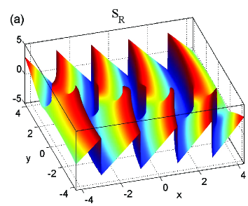
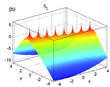
The complex action function displays fascinating features in the complex plane. Decomposing this function into its real and imaginary parts , we write the wave function as . According to this expression, the real and imaginary parts of the complex action determine the phase and amplitude of the wave function, respectively. Figure 3 displays the real and imaginary parts of the complex action for the complex-extended wave function in Eq. (18) at . Figure 3(a) displays the principal zone of the phase of the wave function in the range . Figure 3(b) displays the imaginary part of the complex action in the complex plane. The vanishing of the wave function at nodes indicates that the imaginary part of the complex action tends to positive infinity at nodes. The peaks in Fig. 3(b) correspond to the nodes in the wave function.
The quantized circulation integral around a node in the wave function can be related to the change in the phase of the wave function and this integral can be expressed in terms of the PVF by [67]
| (29) |
where denotes a simple closed curve in the complex plane. The quantized circulation integral around a node of the wave function originates from the discontinuity in its phase. The PVF displays counterclockwise circular flow in the vicinity of a node [67, 68]. Nodes in the complex-extended wave function in Eq. (18) are first-order nodes . As shown in Fig. 3(a), if we travel around a first-order node counterclockwise along a closed path, it follows from Eq. (29) that the phase displays a sharp discontinuity of . Actually, the phase of the wave function is a multivalued function in the complex plane. Thus, if we travel counterclockwise around a node, we then go through the branch cut from one Riemann sheet to another. Through a continuous closed circuit around a node continuing on all the sheet, the phase function generates a helicoid along the vertical axis. Analogous to the case in Bohmian mechanics, phase singularities at nodes in the complex plane can be interpreted as wave dislocations [86, 24].
3.2.3 QMF divergence and vorticity
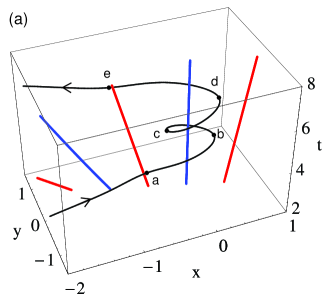
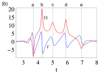
Figure 4(a) shows a trajectory launched from which later arrives at , when maximal interference occurs at , and Fig. 4(b) presents the divergence and vorticity along this trajectory. When the particle approaches a turning point, its velocity undergoes a rapid change and the divergence and vorticity display sharp fluctuations. When the particle approaches the vortical curve at position along the direction of streamline 2 shown in Fig. 1(a), the trajectory displays hyperbolic deflection and the divergence and vorticity display analogous variations, as shown in Fig. 1(c). Around position , when the particle approaches the vortical curve, the positive divergence indicates the local expansion of the quantum fluid. When the particle arrives at the turning points, the divergence vanishes. Then, when it leaves the vortical curve, the negative divergence indicates the local contraction of the quantum fluid. On the other hand, the negative vorticity describes the local clockwise rotation of the quantum fluid.
When the trajectory displays helical wrapping around the stagnation curve, the particle is trapped between two vortical curves. When the particle approaches the turning points and along the direction of streamline 1 shown in Fig. 1(a) and approaches the turning point along the direction of streamline 3, the divergence and vorticity in Fig. 4(b) display analogous variations shown in Fig. 1(b). When the particle approaches and leaves the vortical curve, the divergence describes the local expansion and contraction of the quantum fluid in the vicinity of the vortical curve. The positive vorticity indicates the counterclockwise rotation of the quantum fluid. Finally, when the particle leaves the stagnation curve, it approaches the vortical curve at position along the direction of streamline 4 shown in Fig. 1(a). Again, the divergence and vorticity around position display similar fluctuations shown in Fig. 1(c). Therefore, the variations of the divergence and vorticity around a pole analyzed in Sec. 2.5 provide a qualitative description of the local behavior of the complex quantum trajectories in the vicinity of vortical tubes.
3.2.4 Approximate quantum trajectories
As discussed in Sec. 2.2, the QMF first derivative evaluated at stagnation points determines the local structure around these points [68]. Since it is noted from Eq. (18) that there is always constructive interference at the origin, the origin is a stagnation point at all times. As an example, Fig. 5(a) presents the QMF first derivative at the origin from to . The real part of the QMF first derivative indicates that the QMF displays convergent flow around the stagnation point until . Then, the real part of the QMF first derivative becomes positive and the QMF displays divergent flow. On the other hand, the QMF initially displays clockwise flow around the stagnation point. After , the QMF displays counterclockwise flow. As displayed in Fig. 2, trajectories exhibit helical wrapping around the stagnation curve along from approximately to . During this time interval, the positive imaginary part of the QMF first derivative in Fig. 5(a) describes the counterclockwise flow of the quantum fluid. However, the real part of the QMF first derivative changes sign at . Particles initially converge to the stagnation point and they are gradually repelled by the stagnation point after . Finally, these particles depart from the stagnation point. Therefore, the QMF first derivative at the stagnation point qualitatively explains the behavior of trajectories in the vicinity of the stagnation point.
Additionally, Fig. 5(b) shows that the trajectories starting from the isochrone arrive at the real axis at with the approximate trajectories around the stagnation point given in Eq. (7). Here, the stagnation point in spacetime for Eq. (7) is chosen to be and . The positions for the approximate trajectories are set to be the same as those for the exact trajectories at . As shown in this figure, the trajectory determined by Eq. (7) is a good approximation of the exact trajectory, provided that the approximate trajectory is close to the stagnation point in spacetime.
3.2.5 Wrapping time
These complicated features for trajectories arise from the complex quantum potential in Eq. (11). Both the QMF divergence and vorticity characterize the turbulent flow of complex quantum trajectories. Moreover, the variation of the QMF vorticity provides a feasible method to define the wrapping time for a specific trajectory around a stagnation curve. The wrapping time can be defined by the time interval between the first and last minimum of comprising a region with the positive vorticity. Within this time interval, the positive vorticity describes the counterclockwise twist of the trajectory displaying the interference dynamics, and the stagnation points and poles significantly affect the motion of the particle. For example, Fig. 4(b) indicates that the particle undergoes counterclockwise wrapping around the stagnation curve from to and hence the wrapping time is . Different trajectories have different wrapping times. Therefore, the average wrapping time can be utilized to define the ‘lifetime’ for the interference process observed on the real axis.
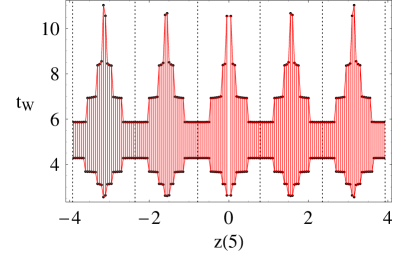
In Fig. 6 we present the wrapping times that correspond to the first and last minimum of the vorticity, which comprise a region with positive vorticity for trajectories launched from the isochrone arriving at the real axis at . Since the process described in Eq. (18) in the complex plane is symmetric with respect to the origin, the data shown in Fig. 6 display the same symmetry. As displayed in Fig. 2(b), trajectories can wrap around stagnation curves with different wrapping times and numbers of loops. Figures 6 and 2(b) indicate that trajectories wrapping around stagnation curves with small rotational radius are trapped between vortical curves for a long time, and this leads to a long wrapping time for these trajectories. On the contrary, if trajectories wrapping around stagnation curves with large rotational radius, when they approach vortical curves, they experience a significant repelling force provided by QMF poles. Thus, these trajectories can easily escape capture by stagnation curves, and this results in a short wrapping time. In addition, it is noted in Fig. 6 that all trajectories display helical wrapping from approximately to . Furthermore, the average wrapping time for these trajectories is , and it can be used to define the lifetime for the interference process in this case.
3.2.6 Rotational dynamics of the nodal line
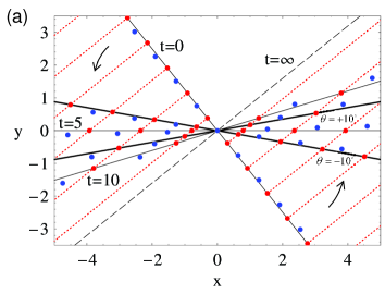
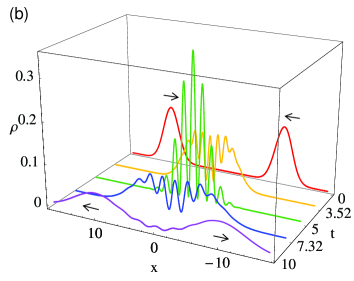
As described in Sec. 3.1, two counter-propagating Gaussian wave packets interfere with each other at all times in the complex plane, and the nodal line rotates counterclockwise with respect to the origin as time progresses. Figure 7(a) shows the evolution of stagnation points and nodes and nodal trajectories in the complex plane, and Fig. 7(b) displays the time-dependent probability densities along the real axis. Initially, the interference of tails of two wave packets contributes to the string of stagnation points and nodes, and the initial nodal line with the angle is perpendicular to nodal trajectories in Eq. (28). Then, the nodal line rotates counterclockwise and lines up with the real axis at . At this time, the total wave function displays maximal interference and the exact nodes form on the real axis. After , these two wave packets start to separate but keep interfering with each other in the complex plane, and the nodal line continues to rotate counterclockwise away from the real axis. Finally, the angle of the nodal line tends to the limit angle when approaches infinity, and the nodal line becomes parallel to nodal trajectories. The rotational rate of the nodal line in Eq. (26) decays monotonically to zero when tends to infinity. In Fig. 7(a), the intersections of the nodal line and nodal trajectories determine the nodal positions, and the distance between nodes in Eq. (27) increases with time. Therefore, the interference process is described by the rotational dynamics of the nodal line with the angular displacement .
In conventional quantum mechanics, interference extrema transiently forming on the real axis are attributed to constructive and destructive interference between components of the total wave function, as shown in Fig. 7(b). In contrast, in the complex quantum Hamilton-Jacobi formalism, the interference features observed on the real axis are described by the counterclockwise rotation rate of the nodal line in the complex plane. Since interference features are observed on the real axis only when the nodal line is near the real axis, we can define the lifetime for the interference process corresponding to the time interval for the nodal line to rotate from to . In Fig. 7(a), the lifetime for the interference features is . Therefore, compared to the conventional quantum mechanics, the complex quantum Hamilton-Jacobi formalism provides an elegant method to define the lifetime for the interference features observed on the real axis.
3.2.7 Quantum caves with Pólya trajectories
Although the QMF displays hyperbolic flow around a node, its associated PVF displays circular flow [67, 68]. Figure 8 shows that Pólya trajectories launched from the isochrone arrive at the real axis with quantum caves. In contrast to Fig. 2(a), these trajectories display helical wrapping around the vortical tubes and hyperbolic deflection around the stagnation tubes. Both the PVF divergence and vorticity vanish everywhere except at poles; thus, trajectories display helical wrapping around irrotational vortical curves described by the PVF.
3.3 Case 2:
Next, we consider the case where the relative propagation velocity is approximately equal to or smaller than the spreading rate of the wave packets. We use the following initial conditions for Gaussian wave packets: , and . Maximal interference also occurs at on the real axis and the propagation and spreading velocities are given by and , respectively.
3.3.1 Quantum caves with quantum trajectories and Pólya trajectories
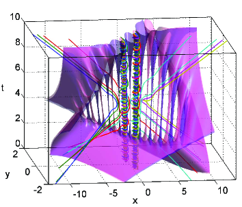
Figure 9 shows that quantum trajectories and Pólya trajectories starting from the isochrone reach the real axis at with quantum caves consisting of the isosurfaces of the wave function and its first derivative. Similar to the case shown in Fig. 2, quantum caves form around stagnation curves and vortical curves appearing alternately, but they are significantly distorted due to the rapid spreading of the wave packets. In addition, quantum trajectories again display helical wrapping around the stagnation tubes and hyperbolic deflection near the vortical tubes. On the contrary, Pólya trajectories display hyperbolic deflection near the stagnation tubes and helical wrapping around the vortical tubes. Again, trajectories launched from different starting points show long-range correlation, and interference leads to the formation of quantum caves and produces complicated behavior of these trajectories.

3.3.2 Rotational dynamics of the nodal line
As shown in Fig. 2, quantum trajectories for Case 1 remain trapped for a certain time interval between vortical curves, and then they depart from the stagnation curves. In contrast, Fig. 9(a) indicates that quantum trajectories can wrap around stagnation curves for an infinite time. This is in agreement with our previous statement that the wrapping time is a measure of the lifetime of the interference features; in this case, these features remain visible asymptotically and the wrapping time becomes infinity.
Figure 10(a) shows the evolution of stagnation points and nodes and nodal trajectories in the complex plane, and Fig. 10(b) displays the time-dependent probability densities along the real axis. The nodal line starting with the initial angle rotates counterclockwise with respect to the origin and reaches the real axis at when the maximal interference is observed on the real axis. Then, the nodal line rotates counterclockwise away from the real axis, and it approaches the limit nodal line with the angle as tends to infinity. Therefore, the nodal line rotates with the angular displacement to reach the limit nodal line parallel to nodal trajectories.
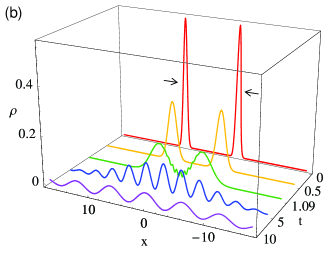
When the nodal line is near the real axis, the interference features are clearly displayed on the real axis. As in Case 1, we can define the starting time of the interference process as the time for the nodal line with the angle . In Fig. 10(a), in this case. In addition, the limit nodal line with the angle is extremely close to the real axis. Therefore, the interference process starts at and remains until tends to infinity. Figure 10(b) indicates that the total wave function starts to display the interference feature when and the interference feature persists at long times.
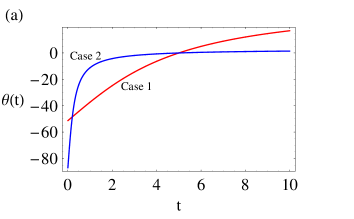
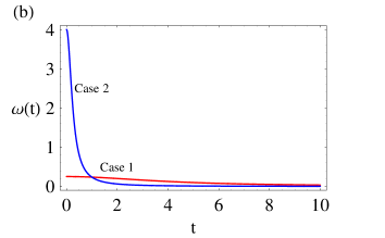
Figure 11 presents the angle and the rotational rate of the nodal line in Eqs. (25) and (26) for Case 1 and Case 2. As indicated in Eq. (26), the rotational rates for these two cases both decay monotonically to zero when tends to infinity. For Case 1, the angle of the nodal line alters relatively slowly and the rotational rate gradually decreases to zero. In contrast, for Case 2, the rotational rate shows a rapid decrease within the initial time interval in Fig. 11(b). This dramatic change in the rotational rate reflects the fast rotation of the nodal line from the initial position to the vicinity of the real axis in Fig. 11(a).
4 Final discussion and concluding remarks
In this study, quantum interference was explored in detail within the complex quantum Hamilton-Jacobi formalism. We reviewed local structures of the QMF and its associated PVF around stagnation points and poles, and derived the first-order equation for approximate quantum trajectories around stagnation points. Analysis of both the QMF divergence and vorticity along streamlines around a pole was employed to explain the complicated behavior of complex quantum trajectories around quantum caves. In addition, both the PVF divergence and vorticity vanish except at poles; hence, the PVF describes an incompressible and irrotational flow in the complex plane. In contrast, both the QMF divergence and vorticity characterize the turbulent flow in the complex plane.
We analyzed quantum interference using the head-on collision of two Gaussian wave packets as an example. Exact detailed analysis was presented for the rotational dynamics of the nodal line on the real axis and in the complex plane. Complex quantum trajectories display helical wrapping around stagnation tubes and hyperbolic deflection around vortical tubes. In contrast, Pólya trajectories display hyperbolic deflection around stagnation tubes and helical wrapping around vortical tubes. For the case where the relative propagation velocity is larger than the spreading rate of the wave packets, during the interference process, trajectories keep circulating around stagnation tubes as a resonant process and then escape as time progresses. Phase singularities in the complex plane can be regarded as wave dislocations. Then, the wrapping time for an individual trajectory was determined by both the QMF divergence and vorticity, and the average wrapping time was calculated as one of the definitions for the lifetime of interference. For the case where the relative propagation velocity is approximately equal to or smaller than the spreading rate of the wave packets, the distortion of quantum caves originates from the rapid spreading of the wave packets. Due to the rapid spreading rate, interference features also develop very rapidly, remaining visible asymptotically in time. The wrapping time becomes infinity, and this implies the infinite survival of such interference features. However, since the interference features are observed on the real axis only when the nodal line is near the real axis, the rotational dynamics of the nodal line in the complex plane offers a unified description to clearly explain transient or persistent appearance of the interference features observed on the real axis. Therefore, these results show that the complex quantum trajectory method provides a novel and insightful interpretation of quantum interference.
The average wrapping time determined by both the QMF divergence and vorticity can be used as one of the definitions for the lifetime of interference. On the contrary, the PVF divergence and vorticity cannot be used to define the lifetime of interference because they vanish except at poles. However, the PVF of a complex function, such as the QMF, contains exactly the same information as the complex function itself [69]. Thus, it is sufficient to define the lifetime of interference as the average wrapping time determined by the QMF divergence and vorticity.
The head-on collision of two Gaussian wave packets with equal amplitudes was used as a model system to explore quantum interference in complex space. This problem is the prototype of quantum systems displaying interference effects, and it also exhibits basic features of quantum interference. A straightforward generalization is to consider the head-on collision of two Gaussian wave packets with different amplitudes. As shown in this paper, these two wave packets interfere with each other in the complex plane for all times. Because of the different amplitudes for these two counter-propagating wave packets, we cannot observe an infinite number of nodes on the real axis. However, nodes can occur on the real axis at specific times. In this case, the nodal line displays not only rotational motion but also translational motion in the complex plane. Analogously, the dynamics of the nodal line in the complex plane clearly explains the interference features observed on the real axis. A detailed analysis will be reported in our future studies.
The current study concentrates mainly on quantum interference arising from the head-on collision of wave packets involving no external potential. We have presented a comprehensive exact analytical study for this problem, and these results demonstrates that the complex quantum trajectory method can provide new physical insights for analyzing, interpreting, and understanding quantum mechanical problems. There are various quantum effects resulting from quantum interference. Therefore, in the future, quantum interference incorporating interaction with external potentials during physical processes can be examined through analytical and computational approaches. Multidimensional problems displaying quantum interference deserve further investigation within the complex quantum Hamilton-Jacobi formalism.
Acknowledgment
Chia-Chun Chou and Robert E. Wyatt thank the Robert Welch Foundation (grant F-0362) for the financial support of this research. A. S. Sanz and S. Miret-Artés acknowledge the Ministerio de Ciencia e Innovación (Spain) for financial support under Project FIS2007-62006. A. S. Sanz also acknowledges the Consejo Superior de Investigaciones Científicas for a JAE-Doc contract.
References
- [1] D. J. Scalapino, in Tunneling Phenomena in Solids, edited by E. Burstein and S. Lundqvist (Plenum Press, New York, 1969), pp. 477–518.
- [2] J. R. Friedman, V. Patel, W. Chen, S. K. Tolpygo and J. E. Lukens, Nature 406, 43 (2000).
- Brumer and Shapiro [2003] P. W. Brumer and M. Shapiro, Principles of the Quantum Control of Molecular Processes (Wiley-Interscience, New York, 2003).
- [4] Atom Interferometry, edited by P. R. Berman (Academic Press, San Diego, 1997).
- [5] D. Leibfried, E. Knill, E. Seidelin, J. Britton, R. B. Blakestad, J. Chiaverini, D. B. Hume, W. M. Itano, J. D. Jost, C. Langer, R. Ozeri, R. Reichle and D. J. Wineland, Nature 438, 639 (2005).
- [6] J. O. Cáceres, M. Morato and A. González-Ureña, J. Phys. Chem. A 110, 13643 (2006).
- [7] A. González-Ureña, A. Requena, A. Bastida and J. Zúñiga, Eur. Phys. J. D 49, 297 (2008).
- Chapman et al. [1995] M. S. Chapman, C. R. Ekstrom, T. D. Hammond, J. Schmiedmayer, B. E. Tannian, S. Wehinger, and D. E. Pritchard, Phys. Rev. A 51, R14 (1995).
- Deng et al. [1999] L. Deng, E. W. Hagley, J. Denschlag, J. E. Simsarian, M. Edwards, C. W. Clark, K. Helmerson, S. L. Rolston, and W. D. Phillips, Phys. Rev. Lett. 83, 5407 (1999).
- [10] C. J. Pethick and H. Smith, Bose-Einstein Condensation in Dilute Gases (Cambridge University Press, Cambridge, 2002).
- [11] J. Javanainen and S. M. Yoo, Phys. Rev. Lett. 76, 161 (1996).
- [12] Y. Castin and J. Dalibard, Phys. Rev. A 55, 4330 (1997).
- [13] M. R. Andrews, C. G. Townsend, H.-J. Miesner, D. S. Durfee, D. M. Kurn and W. Ketterle, Science 275, 637 (1997).
- Shin et al. [2004] Y. Shin, M. Saba, T. A. Pasquini, W. Ketterle, D. E. Pritchard, and A. E. Leanhardt, Phys. Rev. Lett. 92, 050405 (2004).
- Zhang et al. [2006] M. Zhang, P. Zhang, M. S. Chapman, and L. You, Phys. Rev. Lett. 97, 070403 (2006).
- Cederbaum et al. [2007] L. S. Cederbaum, A. I. Streltsov, Y. B. Band, and O. E. Alon, Phys. Rev. Lett. 98, 110405 (2007).
- [17] T. J. Haigh, A. J. Ferris and M. K. Olsen, arXiv:0907.1333v1 (2009).
- [18] T. Schumm, S. Hofferberth, L. M. Andersson, S. Wildermuth, S. Groth, I. Bar-Joseph, J. Schmiedmayer and P. Krüger, Nature Physics 1, 57 (2005).
- [19] P. Böhl, M. F. Reidel, J. Hoffrogge, J. Reichel, T. W. Hänsch and P. Treutlein, Nature Physics 5, 592 (2009).
- [20] R. J. Sewell, J. Dingjan, F. Baumgärtner, I. Llorente-García, S. Eriksson, E. A. Hinds, G. Lewis, P. Srinivasan, Z. Moktadir, C. O. Gollash and M. Kraft, J. Phys. B: At. Mol. Opt. Phys. 43, 051003 (2010).
- [21] J. D. Trimmer, Proc. Am. Phil. Soc. 124, 323 (1980).
- [22] D. Bohm, Phys. Rev. 85, 166 (1952).
- [23] D. Bohm, Phys. Rev. 85, 180 (1952).
- Holland [1993] P. R. Holland, The Quantum Theory of Motion: An account of the de Broglie-Bohm causal interpretation of quantum mechanics (Cambridge University Press, New York, 1993).
- Sanz et al. [2000] A. S. Sanz, F. Borondo, and S. Miret-Artés, Phys. Rev. B 61, 7743 (2000).
- Sanz et al. [2004a] A. S. Sanz, F. Borondo, and S. Miret-Artés, Phys. Rev. B 69, 115413 (2004a).
- Guantes et al. [2004] R. Guantes, A. S. Sanz, J. Margalef-Roig, and S. Miret-Artés, Surf. Sci. Rep. 53, 199 (2004).
- Sanz and Miret-Artés [2007a] A. S. Sanz and S. Miret-Artés, J. Chem. Phys. 126, 234106 (2007a).
- Sanz and Miret-Artés [2007b] A. S. Sanz and S. Miret-Artés, Chem. Phys. Lett. 445, 350 (2007b).
- Sanz and Miret-Artés [2008a] A. S. Sanz and S. Miret-Artés, J. Phys. A: Math. Theor. 41, 435303 (2008a).
- Lopreore and Wyatt [1999] C. L. Lopreore and R. E. Wyatt, Phys. Rev. Lett. 82, 5190 (1999).
- Wyatt [2005] R. E. Wyatt, Quantum Dynamics with Trajectories: Introduction to quantum hydrodynamics (Springer, New York, 2005).
- Poirier [2004] B. Poirier, J. Chem. Phys. 121, 4501 (2004).
- Trahan and Poirier [2006a] C. Trahan, B. Poirier, J. Chem. Phys. 124, 034115 (2006a).
- Trahan and Poirier [2006b] C. Trahan, B. Poirier, J. Chem. Phys. 124, 034116 (2006b).
- Poirier and Parlant [2007] B. Poirier, G. Parlant, J. Phys. Chem. A 111, 10400 (2007).
- Poirier [2008a] B. Poirier, J. Chem. Phys. 128, 164115 (2008a).
- Poirier [2008b] B. Poirier, J. Chem. Phys. 129, 084103 (2008b).
- Park et al. [2008] K. Park, B. Poirier, G. Parlant, J. Chem. Phys. 129, 194112 (2008).
- [40] R. A. Leacock and M. J. Padgett, Phys. Rev. Lett. 50, 3 (1983).
- [41] R. A. Leacock and M. J. Padgett, Phys. Rev. D 28, 2491 (1983).
- [42] M. V. John, Found. Phys. Lett. 15, 329 (2002).
- [43] M. V. John, Ann. Phys. 324, 220 (2009).
- [44] C. D. Yang, Ann. Phys. (N.Y.) 319, 444 (2005).
- [45] C. D. Yang, Ann. Phys. (N.Y.) 321, 2876 (2006).
- [46] C. D. Yang, Chaos Soliton Fract. 30, 342 (2006).
- [47] C.-C. Chou and R. E. Wyatt, Phys. Rev. A 76, 012115 (2007).
- [48] C.-C. Chou and R. E. Wyatt, J. Chem. Phys. 128, 154106 (2008).
- [49] Y. Goldfarb, I. Degani and D. J. Tannor, J. Chem. Phys. 125, 231103 (2006).
- [50] A. S. Sanz and S. Miret-Artés, J. Chem. Phys. 127, 197101 (2007).
- [51] Y. Goldfarb, I. Degani and D. J. Tannor, J. Chem. Phys. 127, 197102 (2007).
- [52] Y. Goldfarb, J. Schiff and D. J. Tannor, J. Phys. Chem. A 111, 10416 (2007).
- [53] Y. Goldfarb and D. J. Tannor, J. Chem. Phys. 127, 161101 (2007).
- [54] B. A. Rowland and R. E. Wyatt, J. Phys. Chem. A 111, 10234 (2007).
- [55] B. A. Rowland and R. E. Wyatt, J. Chem. Phys. 127, 164104 (2007).
- [56] B. A. Rowland and R. E. Wyatt, Chem. Phys. Lett. 461, 155 (2008).
- [57] R. E. Wyatt and B. A. Rowland, J. Chem. Phys. 127, 044103 (2007);.
- [58] R. E. Wyatt and B. A. Rowland, J. Chem. Theory Comput. 5, 443 (2009).
- [59] R. E. Wyatt and B. A. Rowland, J. Chem. Theory Comput. 5, 452 (2009).
- Sanz and Miret-Artés [2008b] A. S. Sanz and S. Miret-Artés, Chem. Phys. Lett. 458, 239 (2008b).
- [61] W. Hänsel, J. Reichel, P. Hommelhoff and T. W. Hänsch, Phys. Rev. Lett. 86, 608 (2001).
- [62] W. Hänsel, J. Reichel, P. Hommelhoff and T. W. Hänsch, Phys. Rev. A 64, 063607 (2001).
- [63] E. A. Hinds, C. J. Vale and M. G. Boshier, Phys. Rev. Lett. 86, 1462 (2001).
- [64] E. Andersson, T. Calarco, R. Folman, M. Andersson, B. Hessmo and J. Schmiedmayer, Phys. Rev. Lett. 88, 100401 (2002).
- [65] K. T. Kapale and J. P. Dowling, Phys. Rev. Lett. 95, 173601 (2005).
- Chou et al. [2009] C.-C. Chou, A. S. Sanz, S. Miret-Artés, and R. E. Wyatt, Phys. Rev. Lett. 102, 250401 (2009).
- Chou and Wyatt [2008b] C.-C. Chou and R. E. Wyatt, J. Chem. Phys. 128, 234106 (2008b).
- Chou and Wyatt [2008c] C.-C. Chou and R. E. Wyatt, J. Chem. Phys. 129, 124113 (2008c).
- Needham [1998] T. Needham, Visual Complex Analysis (Oxford University Press, Oxford, 1998).
- Pólya and Latta [1974] G. Pólya and G. Latta, Complex Variables (John Wiley & Sons, New York, 1974).
- Braden [1987] B. Braden, Math. Mag. 60, 321 (1987).
- Dirac [1931] P. A. Dirac, Proc. R. Soc. A 133, 60 (1931).
- [73] E. A. McCullough, Jr. and R. E. Wyatt, J. Chem. Phys. 51, 1253 (1969).
- [74] E. A. McCullough, Jr. and R. E. Wyatt, J. Chem. Phys. 54, 3578 (1971).
- [75] E. A. McCullough, Jr. and R. E. Wyatt, J. Chem. Phys. 54, 3592 (1971).
- [76] J. O. Hirschfelder, A. C. Christoph and W. E. Palke, J. Chem. Phys. 61, 5435 (1974).
- [77] J. O. Hirschfelder, C. J. Goebel and L. W. Bruch, J. Chem. Phys. 61, 5456 (1974).
- [78] J. O. Hirschfelder and K. T. Tang, J. Chem. Phys. 64, 760 (1976).
- [79] J. O. Hirschfelder and K. T. Tang, J. Chem. Phys. 65, 470 (1976).
- [80] J. O. Hirschfelder, J. Chem. Phys. 67, 5477 (1977).
- Sanz et al. [2004b] A. S. Sanz, F. Borondo, and S. Miret-Artés, J. Chem. Phys. 120, 8794 (2004b).
- [82] C.-C. Chou and R. E. Wyatt, Phys. Rev. A 78, 044101 (2008).
- [83] C.-C. Chou and R. E. Wyatt, Phys. Lett. A 373, 1811 (2009).
- Hirsch et al. [2003] M. W. Hirsch, S. Smale, and R. L. Devaney, Differential Equations, Dynamical Systems, and an Introduction to Chaos (Academic Press, San Diego, 2003).
- Tritton [1988] D. J. Tritton, Physical Fluid Dynamics (Oxford University Press, Oxford, 1988).
- Nye and Berry [1974] J. F. Nye and M. V. Berry, Proc. R. Soc. A 336, 165 (1974).