CONSTRAINING SCALAR FIELD DARK ENERGY WITH COSMOLOGICAL OBSERVATIONS
by
LADO SAMUSHIA
B.S., Tbilisi State University, Georgia, 2002
M.Sc., Tbilisi State University and National Abastumani Observatory, Georgia, 2004
AN ABSTRACT OF A DISSERTATION
submitted in partial fulfillment of the
requirements for the degree
DOCTOR OF PHILOSOPHY
Department of Physics
College of Arts and Sciences
KANSAS STATE UNIVERSITY
Manhattan, Kansas
2009
Abstract
High precision cosmological observations in last decade suggest that about 70% of our universe’s energy density is in so called “Dark Energy” (DE). Observations show that DE has negative effective pressure and therefore unlike conventional energy sources accelerates the cosmic expansion instead of decelerating it. DE is highly uniform and has become a dominant component only recently.
The simplest candidate for DE is the time-independent cosmological constant . Although successful in fitting available data, the cosmological constant model has a number of theoretical shortcomings and because of that alternative models of DE are considered. In one such scenario a cosmological scalar field that slowly rolls down its potential acts like a time-dependent cosmological constant.
I have used different independent cosmological data sets to constrain the time dependence of DE’s energy density in the framework of the slowly-rolling cosmological scalar field model. Present data favors a time-independent cosmological constant, but the time-dependent DE can not be ruled out at high confidence level. Ongoing and planned cosmological probes and surveys will provide more and better quality data over the next decade. When the new data sets are available we will be able to either detect the time dependence of DE or constrain it to a very small physically uninteresting value.
CONSTRAINING SCALAR FIELD DARK ENERGY WITH COSMOLOGICAL OBSERVATIONS
by
LADO SAMUSHIA
B.S., Tbilisi State University, Georgia, 2002
M.Sc., Tbilisi State Unviersity and National Abastumani Observatory, Georgia, 2004
A DISSERTATION
submitted in partial fulfillment of the
requirements for the degree
DOCTOR OF PHILOSOPHY
Department of Physics
College of Arts and Sciences
KANSAS STATE UNIVERSITY
Manhattan, Kansas
2009
Approved by:
Major Professor
Bharat Ratra
Acknowledgments
I am grateful to so many people for their help and support while writing this thesis and during my entire graduate studies. I am indebted to my research adviser Professor Bharat Vishnu Ratra who was supervising my research activities. Thank you for your help, guidance and patience, It has been my great honor to have worked with you. Special thanks to Professor Tina Kanhiashvili, its mainly due to her suggestion and help that I joined Kansas State University as a graduate student. Whenever I had a question in physics or mathematics I knew that I could always talk to Professor Larry Weaver, he taught me more than I could read in any reference book on physics. Many thanks to Professors Tim Bolton and Glenn Horton-Smith whom I bugged whenever I had a question about statistics. Professors Victor Turchin and David Aukley were always willing to help and answer my rookie mathematical questions. I am very grateful to Dale and Maureen Herspring for hospitality during my first weeks in Manhattan. Special thanks Brad and Susie Shaw, your beautiful friendship made us feel more like home. My dear friends and fellow graduate students from physics department, I will always remember wonderful times spent with you. And of course, many many thanks to my wife Nino and daughter Nutsa, you made my life beautiful.
Dedication
To the memory of my loving mother.
Chapter 0 Introduction
1 Short overview of relevant topics from theoretical cosmology
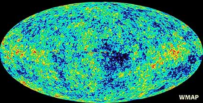
Observations suggest that our Universe started evolving from an extremely hot and dense state to ago. Since light travels at finite speed, the distance to which we can see is fundamentally limited. The observable Universe today has a Hubble radius of about , beyond which we can not see. Astronomical observations show that, on average, our Universe is homogeneous and isotropic on large scales. Observational evidence for isotropy includes the measurement of cosmic microwave background radiation anisotropies [1], shown in Fig. 1, that is very isotropic.
Large-scale structure observations confirm that the galaxy distribution becomes homogeneous beyond about , but even on the largest observed scales inhomogeneities in galaxy density are on the order of a few percent [2].
Homogeneous and isotropic four dimensional space-times are described by the metric
| (1) |
where is cosmic time and is the metric of the three-space which can be flat, spherical, or hyperbolic. is called a scale factor and describes how the spatial separation between two noninteracting test particles changes with time. In an expanding Universe the scale factor is an increasing function of cosmic time.
In general relativity (GR), the metric obeys Einstein’s equations
| (2) |
where is Newton’s gravitational constant, is the Ricci tensor,
| (3) |
and the Christoffel symbols are given by
| (4) |
in Eq. (2) is the energy-momentum tensor of the matter components that fill space. The Ricci tensor satisfies the Bianchi identity , where the semicolon denotes a covariant derivative, and consequently the energy-momentum tensor satisfies the energy conservation equation
| (5) |
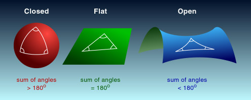
Three-dimensional homogeneous and isotropic space can be flat, positively curved (surface of a 3-dimensional “sphere”), or negatively curved (surface of a 3-dimensional “saddle”); two dimensional analogs are shown in Fig. 2.
The metric of homogeneous and isotropic space can be written in Cartesian coordinates as
| (6) |
and in spherical coordinates as
| (7) |
Here is the Kroneker delta function and . describes the geometry of three-space. For the space is negatively curved (open), for the space is positively curved (closed), and for the space is flat. The variable is given by
| (8) |
The numerical value of depends on the normalization of the scale factor. In open and closed Universes is usually normalized in such a way that . In the spatially-flat Universe the scale factor is often normalized so that it’s current value is equal to .
If the metric is given by Eqs. (1) and (7) than Eq. (2) forces the energy-momentum tensor to have the form
| (9) |
where is the mass energy density of matter and is pressure.
For barotropic fluids pressure depends only on the local value of energy density, . Very often the equation of state is used, where is called the equation of state parameter. For an ultrarelativistic gas (radiation) , for nonrelativistic matter , and for a cosmological constant .
Energy conservation, Eq. (5), in the expanding Universe gives
| (10) |
For a general barotropic fluid Eq. (10) can be solved and yields
| (11) |
which for becomes
| (12) |
where is the current energy density of the fluid.
The combination is known as the Hubble parameter, where an overdot denotes a derivative with respect to cosmic time . It shows how fast the Universe is expanding. Its current value is called the Hubble constant and is often quoted in terms of a dimensionless parameter .
In the Universe described by Eqs. (1) and (7) and dominated by a single barotropic fluid, Eq. (2) reduce to two independent equations for the scale factor
| (13) | ||||
| (14) |
Equation (10) follows from Eqs. (13) and (14). In the Universe dominated by a single barotropic fluid, Eqs. (13) and (14) give
| (15) |
Equation (13) shows that if the curvature is zero. This time-dependent energy density that makes the Universe spatially-flat is called the critical density. Current energy densities of matter components are often given in terms of dimensionless density parameter, .
In a curved space with radiation, nonrelativistic matter, and cosmological constant Eq. (13) can be rewritten as
| (16) |
where , , , and are respectively the density parameters of nonrelativistic matter, radiation, cosmological constant, and curvature, and the scale factor is normalized so that .
2 Distance and time measurements in cosmology
Distances can be measured directly, using the parallax method, only to astronomical objects that are close to us (less than 100 ). For objects that are farther away indirect methods of distance determination must be used.
When a distant object emits a photon with a wavelength at time , since light travels at finite speed, we will detect the photon at a later time . As the Universe expands, the photon will “redshift” and we will detect it at a longer wavelength
| (17) |
where and are respectively scale factors at the moment of emission and detection (now) of the photon. Redshift of an astronomical object is defined as
| (18) |
where is the value of the scale factor at the moment when the light that reached us from that body was emitted.
If the cosmological expansion history is known, redshift can be uniquely related to the distance to the object and the time of light’s emission. Distances and times in cosmology are often quoted in terms of redshifts. Two most frequently used distance measures in cosmology are the luminosity distance and the angular distance.
1 Measuring time intervals
Light travels on null geodesics . When we detect a photon that was emitted at redshift it has traveled for time , where is the distance and is speed of light. Let’s set up the coordinate system so that the photon travels in the radial direction. Then from Eqs. (1) and (7) the total elapsed time can be expressed as
| (19) |
Using Eq. (16) and the identities and , we can rewrite Eq. (19) as
| (20) |
In a given cosmological model Eq. (20) uniquely relates redshift to time.
2 Luminosity distance
Let’s say we have a source of known luminosity (power) at a redshift . The source emits energy in a time interval and this energy redshifts by before it reaches us. The energy is distributed over a spherical surface with radius , where is the distance that a photon travels before detection. The flux that we measure in unit time interval is given by
| (21) |
Luminosity distance is defined as
| (22) |
By substituting from Eq. (20), the luminosity distance can be rewritten as
| (23) |
Luminosities of some astronomical objects can be determined by indirect measurements. Supernovae Type Ia (SNeIa), for example, have very small dispersion in total luminosity. Gamma-ray bursts (GRBs) could be well calibrated in the future with their luminosity determined to high accuracy. We can measure the flux of these and other “standardizable candles” at different redshifts to determine cosmological parameters from Eq. (23).
3 Angular diameter distance
Let’s say an astronomical body at a distance from us has a physical size , then the observed angle subtended by that body is . The angular diameter distance is defined as
| (24) |
If the object is at redshift it will span the angle . Using arguments of Section 2 we can express the angular diameter distance through cosmological parameters as
| (25) |
Similarly to standard candles, “standard rulers”, such as FRII radio galaxies, have small dispersion in physical size. Equation (25) then can be used to determine cosmological parameters from the redshifts and apparent angular sizes of those standard rulers.
3 Short overview of relevant topics from observational cosmology
In last decade the quality and quantity of astronomical observations relevant to cosmology have greatly improved. SNeIa can map the expansion of the Universe up to the redshift of 1.7 (see Fig. 3). While the power spectra of CMB anisotropies (see Fig. 4) and the galaxy distribution (see Fig. 5) have been measured to a high precision.
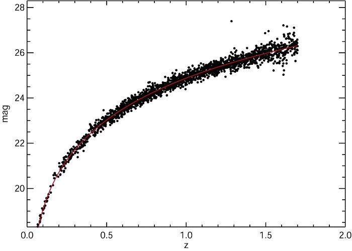
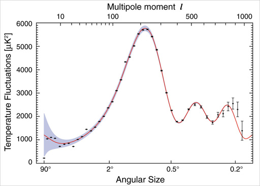
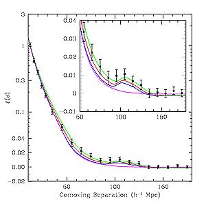
The combination of SNeIa absolute magnitude versus redshift data [3, 4], measurements of CMB anisotropy [5], cluster gas mass fraction versus redshift data [6], measurements of the baryon acoustic peak [7, 8], and other large-scale structure measurements [9] can be used to determine cosmological parameters with high precision.
Currently available cosmological data strongly indicate that:
-
•
The Universe is highly isotropic and homogeneous.
-
•
The Universe is expanding and distance between gravitationally unbound objects are increasing.
-
•
The cosmic expansion started accelerating at a redshift near , if the dark energy is a cosmological constant.
-
•
The spatial curvature of the Universe is very close to zero, if the dark energy is cosmological constant.
The accelerated expansion of the Universe can be understood if we assume that around of the current cosmological energy budget is made of dark energy (DE). Parameterized as a fluid, DE has a negative equation of state parameter and is spatially uniform.
About the other matter components we know that:
-
•
The Universe is filled with CMB photons. The CMB has an accurately Plankian spectrum with a temperature of . Radiation today makes a negligible contribution to the total energy density.
-
•
Baryons make up less than 5% of critical density. About 75% of baryonic matter is Hydrogen, 25% Helium. Contribution of heavier elements to the total baryonic energy density is small. The entropy of the Universe is high, around photons per baryon.
-
•
Nonrelativistic, cold dark matter (CDM) contributes around 25% of the critical density. CDM is not baryonic and does not significantly emit, absorb, or scatter light.
A joint analysis of current CMB anisotropy measurements, SNeIa data, and BAO peak measurements results in the following 1 ranges for key cosmological parameters [10]:
-
•
.
-
•
.
-
•
.
-
•
.
-
•
Age of the Universe = Gyr.
Chapter 1 Dark Energy
1 Observational evidence for dark energy
The first direct evidence of accelerated expansion was provided by SNeIa absolute magnitude versus redshift data [16, 17]. Accelerated expansion is very difficult to explain in GR with only conventional matter. Equation (14) implies that the expansion can be accelerating only if the Universe is dominated by a component with negative pressure . The initial SNeIa measurements were followed by ground-based and space surveys, such as the Hubble Space Telescope (HST) survey [18], the supernova legacy survey (SNLS) [19], and the ESSENCE survey [20]. Current SNeIa data extends to and provides more than 5 evidence for accelerated expansion.
Positions and amplitudes of acoustic peaks in the CMB anisotropy show that the Universe is very close to spatially flat if DE does not evolve in time. When CMB anisotropy results are combined with an independent measurement of the Hubble constant they indicate that nonrelativistic matter makes up only about a quarter of the critical density, while the energy density of radiation is negligible. This implies that about three quarters of our Universe’s energy budget is made of something different than ordinary or dark matter and radiation. This extra component must be uniform on cosmological scales and became dominant recently, in order not to adversely effect large-scale structure formation and big bang nucleosynthesis.
The presence of DE also effects CMB anisotropies directly through the integrated Sachs-Wolf (ISW) effect. In a Universe dominated by DE gravitational wells decay on large distance scales. This affects the large-angle CMB spectrum, since photons that travel through decaying gravitational potentials gain energy. If the Universe is dominated by DE there should be cross-correlation between CMB anisotropies and low-redshift matter distribution. Several groups reported detection of the ISW effect in cross-correlations of the CMB with galaxy and radio-source catalogs [21, 22, 23].
These results, combined with the BAO peak measurements, LSS tests, and galaxy cluster data, provide fairly overwhelming evidence that about of the current Universe’s budget is in spatially uniform DE with negative pressure.
2 CDM model
All currently available cosmological data is quite consistent with a Universe that is spatially-flat, is dominated by a cosmological constant with , with the rest of the energy density being in nonrelativistic cold dark matter with and nonrelativistic baryonic matter with . A cosmological constant has and according to Eq. (10) it’s energy density does not change in time. This model is referred to as the “standard model” or the spatially-flat CDM model.
In the spatially-flat CDM model the background expansion of the Universe at late times is described by
| (1) |
Although the CDM model is a good fit, the data is not yet tightly constraining and does not yet require a constant . To account for the possibility of a time-varying cosmological constant the equation of state of DE is sometimes modeled as , where is a negative parameter. This, so called, XCDM parametrization lacks physical motivation. XCDM is usually used as an ansatz in data analysis for the purposes of quantifying time-dependence of DE.
3 Problems of CDM
Although successful in fitting most data, the CDM model has a number of theoretical shortcomings. A cosmological constant is difficult to motivate from fundamental physics. The most plausible candidate for a cosmological constant is vacuum energy.
Since all Lorentz observers should see the same vacuum, it’s energy-momentum tensor must be proportional to the metric tensor . The vacuum therefore has the required equation of state . It’s very difficult however, to explain the small value of DE energy density based on the vacuum energy model.
In the quantum field theory the zero point energy of the vacuum is divergent
| (2) |
Quantum field theory is expected to break down at the Planck scale of around . If we use this as upper integration limit in Eq. (2) (instead of ) we get a huge number that exceeds the observed dark energy density by 120 orders of magnitude.
In a supersymmetric model every boson has a fermion of equal mass as a supersymmetric partner and the vacuum energies of these partners cancel. Supersymmetry (SUSY), if existent, is believed to be broken at an energy of roughly or so. If we cut off the upper integration limit in Eq. (2) at the energy of SUSY breaking we will still get a difference of around 60 orders of magnitude. This discrepancy between the small measured value of cosmological constant and the much larger theoretically “expected” values of vacuum energy is known as the “smallness” problem [24].
One possible explanation of the “smallness” problem is based on anthropic arguments. In string theory, multiple vacuum states with all possible values of vacuum energy are possible. Different causally disconnected patches of the Universe spontaneously choose vacuum states that are independent of each other. If the Universe is infinite there will always be parts of it that have a given value, no matter how unlikely, of the vacuum energy and we just happen to live in one of those regions with a very small value of vacuum energy density [25, 26].
Another interesting fact that’s difficult to explain in the CDM model is that today both nonrelativistic matter and DE have comparable energy densities. This is surprising since the matter and DE components scale with redshift differently. For radiation it is , for CDM and baryons , and for a cosmological constant .
At the beginning of cosmic evolution the Universe was radiation dominated, today radiation contributes less than 1% of the total energy density. The contribution of DE was negligible in the past, it has become a dominant component only recently, and in the future will be the only component driving cosmic expansion as shown in Fig. 1.
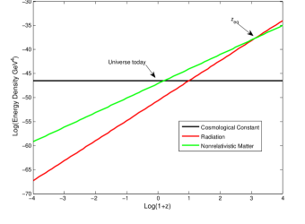
There is only a short period of time when the energy densities of matter and cosmological constant are comparable. It is unclear why we happen to live in this narrow window of time. This is called the “coincidence” problem and like the “smallness” problem can be addressed by the anthropic arguments.
Besides the two problems mentioned above there are other observational facts that appear to conflict with the predictions of the CDM model, at possibly more then 2 confidence level. These are
-
•
High redshift SNeIa data are consistent with spatially-flat CDM. It favors however models with . Initially, this was thought to be a statistical fluke that would go away as more data accumulated. This discrepancy however still persists even as larger data sets become available. The discrepancy is caused by high () redshift SNeIa which are systematically brighter than what we would expect in the CDM model [3]. This could be due to an unknown systematic effects, possibly associated with high-redshift SNeIa evolution, or a statistical effect that will go away with more data. If the discrepancy persists, it would mean that the Universe in the past was decelerating faster than the CDM model predicts.
-
•
Large-scale velocity flows have amplitude of , larger than what is expected in a CDM model [27, 28, 29, 30, 31]. Velocity flows extend to and could be as large as . In CDM the probability of having velocity flows with such a large amplitude is less then 1%. The explanation for this could be that it is just a big statistical fluctuation or there could be some physical reason, such as time-dependent Newton’s constant, presence of noninflationary perturbations, or a giant void at a distance of few Gpc.
-
•
Cosmological simulations based on the CDM model predict that large voids should be filled with many dwarf dark matter halos. This turns out to be true for very large voids (larger than ). Smaller voids however are observed to be surprisingly empty of dark matter halos [32]. For example, based on CDM we would expect to observe on average 10 dwarf galaxies in our local void, but there are none. Possible resolution of this problem could be related to the incompleteness of observational sample, or incorrect bias model that fails to account for specific environmental properties.
At the moment these discrepancies between observations and theoretical predictions do not have big weight in the overall picture. The CDM model is in general a good statistical fit to the combined data. These inconsistencies might go away when new high-quality data become available.
4 Alternative dark energy models
At the moment, CDM is a good fit to available cosmological data, however, because of the observational issues mentioned in Sec. 3 and its inability to naturally account for the small observed energy density of DE, a number of alternative models have been proposed over the years.
One approach is to not introduce a new exotic DE component, but to modify the equations of GR and consequently Eq. (2), [33, 34, 35, 36, 37]. In this set of models gravity is usually weaker on larger scales and the accelerated expansion is just a gravitational effect. At very early times modified gravity should act like GR predicts, in order not to conflict with predictions of CMB anisotropy and BBN. In and scalar-tensor theories, the equivalents of Eq. (2) include up to forth order derivatives of the metric tensor. Gravity is not a spin-2 transverse and traceless field anymore. It is also carried by spin-0 (scalar) and spin-1 (vector) particles.
Another possibility is that the Universe is not as homogeneous as we thought and the accelerated expansion is an effect of averaging nonlinear spatial inhomogeneities over cosmological scales [38, 39, 40, 41]. It is not yet clear if the backreaction of structure formation on the background evolution can be strong enough to mimic accelerated expansion and at the same time be consistent with all other available data.
A third option is to introduce a DE fluid that is close to spatially uniform but unlike a cosmological constant slowly varies in time. This is usually achieved by introducing a scalar field that is slowly rolling down it’s almost flat potential [42, 43]. In the minimal model, the scalar field is coupled to the rest of the matter only gravitationally, but other couplings have also been considered [44, 45, 46, 47].
Chapter 2 Cosmological Scalar Field
1 Scalar field in the expanding universe
Let’s assume that a self-interacting scalar field minimally coupled to gravity is present on cosmological scales. This scalar field is described by the lagrangian density
| (1) |
where is the potential energy density. The energy momentum tensor of this scalar field is given by
| (2) |
If the scalar field is close to spatially uniform on cosmological scales we can neglect its spatial derivatives compared to time derivatives and the individual components of the homogeneous part of the energy momentum tensor can be written as
| (3) | ||||
| (4) | ||||
| (5) | ||||
| (6) |
By looking at Eqs. (5) and (6) we can see that the equation of state parameter
| (7) |
can become negative if the scalar field evolves slowly in time. The equation of state parameter is always greater than and in the limit of the scalar field “at rest” () we effectively get a cosmological constant with .
The time evolution of the scalar field (and consequently the time evolution of the equation of state parameter) is determined by the Klein-Gordon equation. For the metric given by Eq. (1) the Klein-Gordon equation is
| (8) |
If the scalar field energy density makes nonnegligible contribution to the total energy budget of the Universe it will affect the evolution of the scale factor and Eq. (16) should be rewritten as
| (9) |
where is now the time-dependent energy density parameter of the scalar field.
To make specific predictions about how the scalar field affects the Universe’s evolution we have to specify the form of the potential . Since the underlying physics is not known at the moment, it’s impossible to pick a specific functional form for based on the considerations of fundamental physics only.
The only fundamental scalar field in the standard model of particle physics is the Higgs field. Rest mass of the Higgs boson is larger than about and at low energies it decays into bosons, , therefore Higgs bosons can not be present in large quantities in the late universe. In the theories that go beyond the standard model, such as string theory, minimal supersymmetric theory, etc., fundamental scalar fields arise naturally and we have a large number of candidates. The particle physics at very high energies is not well constrained experimentally yet and different theoretical scenarios are possible; because of this uncertainty its impossible to motivate one choice of potential based on fundamental considerations and a number of different models have been proposed over the years. An incomplete list of possible scalar field potentials is shown in Table 1.
| Potential | Reference |
|---|---|
| [42] | |
| [43] | |
| [52] | |
| [53] | |
| [54] | |
| [55] | |
| [56] |
In this work I will concentrate on the inverse-power law potential first proposed in Ref. [42]. In this model the potential is assumed to be inversely proportional to a power of the scalar field, , where is a positive constant.
2 Inverse-power law potential
If we take scalar fields self-interaction potential to be inversely proportional to a power of ,
| (10) |
where and are nonnegative parameters, Eqs. (9) and (8) can be rewritten as
| (11) | |||
| (12) |
where we have set spatial curvature to zero and neglected radiation, and the energy density of the scalar field is given by
| (13) |
Parameter describes the steepness of the scalar field potential. Larger values of correspond to faster evolution of the scalar field and vice versa. corresponds to the time-independent cosmological constant. Parameter sets the mass scale of the scalar particle,
| (14) |
In the distant past, when the energy density of the scalar field is much less than the energy density of other components , Eq. (12) accepts a solution
| (15) |
and the equation of state parameter of the scalar field is
| (16) |
For positive , redshifts less rapidly than the dominant component of energy and at some point eventually starts to dominate. The redshift when cosmic acceleration starts is given by
| (17) |
As we approach , the fractional energy density of the scalar field increases and the approximation breaks down. Evolution of the scalar field does not follow Eq. (15) anymore and to solve for now the set of coupled differential equations (11) and (12) must be solved numerically.
A nice property of Eq. (15) is that it is an attractor. A wide range of initial conditions on result in solutions that converge to the solution of Eq. (15) at some point. Figure 1 shows the evolution of the scalar field for different initial conditions. Although initial conditions on span some 70 orders of magnitude, the late-time evolution of the scalar field is similar in all intermediate cases.
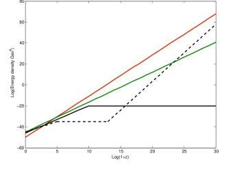
In the scalar field scenario the “smallness” and “coincidence” problems mentioned in Sec. 1 are partially solved. The scalar field can start from a very high energy state, roll down the inverse power law potential, and naturally lead to a that evolves to the very small measured value. Figure 1 shows that the scalar field “tracks” the evolution of the dominant component once it joins the solution of Eq. (15). The energy densities of nonrelativistic matter and scalar field are comparable for a longer period of time, and current time becomes less special.
The scalar field in this model does not cluster on scales much smaller than the Hubble radius as required by CMB and large-scale structure data.
3 CDM model of dark energy
In our analysis we will assume that the only two constituents affecting the late-time evolution of the Universe are nonrelativistic cold dark matter and baryons with energy density parameter and a scalar field with inverse power law self-interaction potential . We will also assume that the Universe is spatially-flat which implies .
In this model the background expansion is fully described by two parameters, and . The evolution of the scale factor and scalar field are governed by
| (18) | |||
| (19) |
For the CDM model reduces to the spatially-flat CDM with . For nonzero predictions of CDM and CDM differ, for example the scalar field model predicts lower values of luminosity and angular diameter distances for the same value of Hubble parameter and nonrelativistic matter density. An example of a C++ function that solves Eqs. (18) and (19) is presented in Appendix 9.
Different cosmological tests have been used in the past to constrain the parameters of the CDM model, including counts of galaxies [57], angular sizes of radio sources and quazars [58, 59], galaxy cluster gas mass fraction data [60], strong gravitational lensing [61] and SNeIa absolute magnitude versus redshift data [62, 63, 64]. In next chapters I will discuss the constraints on CDM model from some current data sets.
Chapter 3 Data Analysis Techniques
We are interested in observable quantities measured at redshifts (or in redshift bins of width ). could be, e.g., luminosity distance, angular diameter distance, Hubble parameter, or quantities that implicitly depend on them. First I will assume that evolution of the Universe is described by the CDM model, as presented in Chapter 2, with unknown values of parameters and . For given values of model parameters we can compute the theoretical expectations for the observed quantities. We will find the best-fit parameters and , for which the theoretical predictions are the closest match to the results of observations by some measure. We will also construct the confidence level intervals that are likely to cover the true values of parameters with a specified probability.
We will compare the predictions of CDM model to the ones of CDM and see which ones fit the observations best. In the end we will see if data favors one model over the other, and quantify the degree of discrepancy between the two models.
1 and likelihood functions
Let’s say we have measurements at redshifts with measurement errors , and the CDM model predicts . The function,
| (1) |
quantifies the discrepancy between theoretical predictions and observations. Small values of indicate a good fit. The parameters and that minimize are called the best-fit parameters. The likelihood function,
| (2) |
has a local maximum at (, ). If the measurements are independent and Gaussian distributed with mean and variance , then the best-fit values of parameters are unbiased estimators of their true values. Values of parameters that result in high values of the likelihood function are more likely to be the true parameters.
1, 2, and 3 confidence level contours are defined as the pairs of parameters (, ) for which is less by 2.30, 6.18, and 11.83 respectively compared to . If the likelihood function had an exact two dimensional Gaussian profile,
| (3) |
N contours would correspond to the range of parameters . In that case the 3 contour would enclose 99.73% of integrated likelihood and the parameter values outside that range would be 0.27% or less likely to be the true parameters. This is not true for an arbitrary , however, when it is a sharply peaked function, parameter values outside 3 are usually less than 1% likely.
2 Nuisance parameters
Very often will depend on parameters other than and . These “nuisance” parameters can be determined from the data but are of no interest to us. Examples of nuisance parameters in dark energy parameter estimation are the Hubble constant and baryonic energy density parameter . In this case the likelihood function will also depend on . If we have some idea from other observations about what the values of are, we can summarize this information in the form of probability distribution function (p.d.f.) . is normalized to one and is usually taken to be a Gaussian peaked at the best-fit value of determined from other independent data sets. If we do not want this implicit use of information from other data sets, we can use the conservative flat prior over the range . We then integrate the likelihood function,
| (4) |
and determine the best fit values and confidence level contours from as in Sec. 1.
Two most frequently used priors on the Hubble constant are the measurement of Hubble Space Telescope (HST) team [67] and the result from the Wilkinson Microwave Anisotropy Mission (WMAP) 5-year data [68] . The WMAP measurement has less dispersion but is model dependent, unlike the HST measurement which measured directly based on the recessional speeds of distant objects. The most conservative option is to integrate over with a flat, noninformative prior. The baryonic matter energy density is also well constrained by a number of independent tests. Big bang nucleosynthesis gives the value [69] and the WMAP data results in .
3 Constraints on individual cosmological parameters
One-dimensional confidence level contours and best-fit values can be computed for individual cosmological parameters and . We take the two-dimensional likelihood function from Eq. (4) and integrate it with respect to the other parameter with a flat prior.
| (5) | ||||
| (6) |
For each parameter we find the best-fit value that maximizes the corresponding one-dimensional likelihood function. We define 1, 2, and 3 confidence level intervals and () so that
| (8) | ||||
| (9) |
and equals to 68.27, 95.45, and 99.73 respectively. We will choose lower and upper limits on parameter values so that the likelihood is higher everywhere inside the interval than outside.
Parameter should always be positive. Since the best-fit values are usually close to the line, in Eq. (8) will often be equal to zero.
Chapter 4 Constraints on CDM from Hubble Parameter Measurements
1 Hubble parameter measurements
The Hubble parameter in spatially flat CDM is given by
| (1) |
and is a function of redshift and cosmological parameters and . In practice, it can be measured indirectly at different redshifts and thus used to constrain cosmological parameters of interest.
First of all let’s note that since , the Hubble parameter can be rewritten as
| (2) |
Equation 2 shows that the Hubble parameter can be determined from the measurement of . itself can be determined from a survey that measures redshifts of galaxies with high precision. The basic idea is that if we have two galaxies very close in redshift space and we can determine their ages with good accuracy, then can be approximated by reasonably well with , where is the difference in their redshift and is the difference in their age. The most difficult part is to accurately determine ages of galaxies.
In passively evolving galaxies the star formation rate is low and their ages can be determined with better accuracy. These galaxies are dominated by the light from old red main sequence stars. The evolution of those stars is a well understood process and metallicity can be simulated on computers. The spectra of galaxies depends mainly on metallicity and age. A computed spectrum can be compared to the observed one and the galaxy age can be determined. Stars in galaxies, of course, do not have the same metallicities and this spread in metallicity introduces a statistical error of about . For a detailed description of this and other relevant issues and methods see Refs. [73].
2 Constraints from Hubble parameter data
Reference [74] used Gemini Deep Deep Survey [75] and archival data [76, 77, 78, 79, 80] to estimate ages of 32 passively evolving galaxies. From these age measurements they were able to compute the differential age at 9 different redshifts in the redshift range . The age measurements are shown in Appendix 10, while the Hubble parameter estimates from Ref. [74] are shown in Appendix 11. These measurements are independent and the errors are Gaussian distributed. The function is
| (3) |
where is the theoretical value of Hubble parameter computed from Eq. (1), and and are the observed values and one sigma uncertainties. In our analysis we assume 12% uncertainties on age measurements in Appendix 10 [81].
The Hubble constant (the Hubble parameter now, at zero redshift) is a nuisance parameter and can be integrated over to get a two dimensional likelihood function of cosmological parameters
| (4) |
where is a prior probability distribution function for . We integrate over with a Gaussian WMAP prior with .
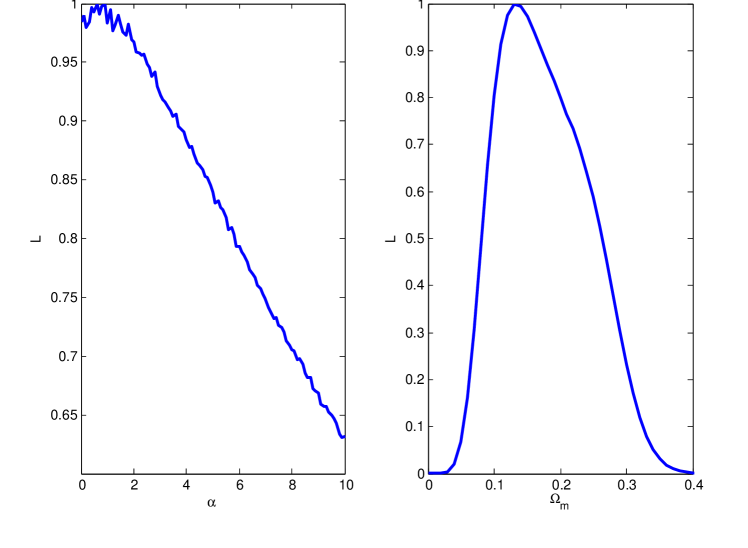
The 1, 2, and 3 contours on CDM are shown in Fig. 1. Data constrain the nonrelativistic matter density parameter to be less than 0.4 at about 3 confidence level. The likelihood in the direction of is almost flat. The one dimensional likelihood functions on individual dark energy parameters are shown in Figure 2. is poorly constrained while the nonrelativistic matter density parameter is constrained to be in the range at 1.
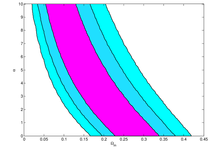
3 Lookback time
The data in Appendix 10 can be used to directly constrain dark energy parameters using the lookback time versus redshift relation [82, 83, 84, 45, 85, 86, 87, 88, 89]. Lookback time at redshift is defined as the difference between the current age of the Universe and it’s age at redshift . In CDM the lookback time is given by
| (5) |
For an object at redshift it’s age is the difference between the Universe’s age at and the one when the object was formed at redshift .
| (6) |
From Eqs. (5) and (6) the observed lookback time is defined as
| (7) |
where is observed total age of the Universe, is the objects age at redshift , and is a “delay factor” that encodes our ignorance of . The “delay factor” is different for each object in the sample. From CMB experiments the total age of the Universe is estimated to be [68].
We construct the function
| (8) |
and compute the likelihood function
| (9) |
We account for our ignorance of by marginalizing over it by integrating the likelihood function in Eq. (9) analytically over with a flat prior.
| (10) |
where
| (11) | ||||
| (12) | ||||
| (13) | ||||
| (14) |
and is the complementary error function. Finally we integrate over the Hubble constant with a Gaussian WMAP prior with to get the constraints on CDM model parameters and .
4 Constraints from lookback time versus redshift data
The constraints on CDM from the lookback time method are shown in Fig. 3.
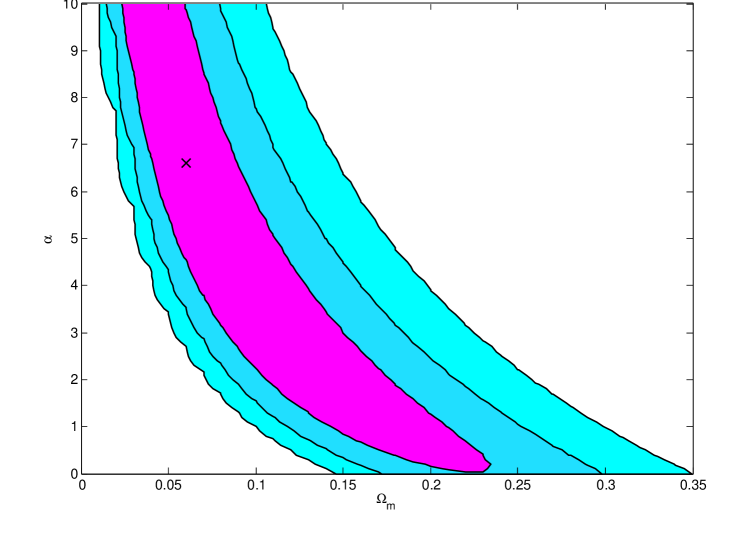
Lookback time versus redshift data constrains the nonrelativistic matter density to be less than at about 3 confidence level. The parameter is not well constrained and values as large as are allowed at 1 confidence level. The best fit parameters from the two dimensional likelihood function are and .
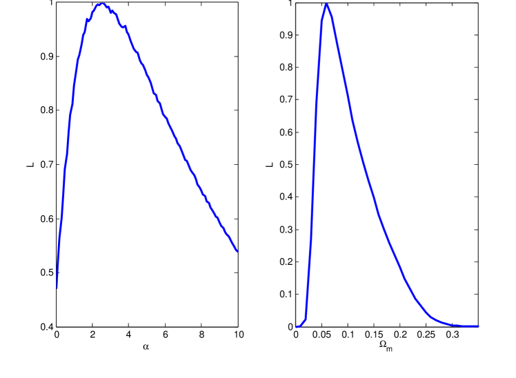
The one-dimensional likelihoods of individual cosmological parameters are shown in Fig. 4. The best fit values are and . The 1 intervals are and .
At the moment lookback time versus redshift and Hubble parameter versus redshift measurements can not provide strong constraints on cosmological parameters. Both data sets are expected to improve significantly in the near future [81]. The updated data sets in combination with other measurements might prove to be very useful in constraining cosmological parameters.
Chapter 5 Constraints on CDM from SNeIa and GRB Data
1 Supernova Type Ia as standard candles
Supernovae (SNe) are highly luminous objects. At the peak of their activity SNe can be as bright as an average galaxy. They reach maximum brightness shortly after the stellar explosion and then slowly fade away in several weeks. The shock wave from explosion pushes a spherical shell of gas and dust into the interstellar medium and leaves behind a visible SNe remnant. SNe are classified based on the absorption lines of chemical elements in their spectra. SNe that do not have hydrogen atom Balmer lines in their spectra are classified as Type I, while those that have Balmer lines belong to type II. SN can be farther divided into subtypes. SNe type Ia (SNeIa) for example lack hydrogen lines but have a singly ionized silicon (Si II) line at . SNeIa are the most useful for cosmological parameter estimation. First of all, they are astonishingly bright and can be seen at large distances. Secondly, they are very homogeneous in spectra, light-curve shapes, and peak absolute magnitude and can be easily calibrated and used as standard candles.
SNeIa are believed to be carbon-oxygen white dwarfs in a binary system. The white dwarf accretes matter from its companion until it reaches the Chandrasekhar mass limit of 1.4 solar masses. As the density and temperature inside the star increases, the mass in the core undergoes nuclear fusion, which results in a SNeIa explosion. The masses of white dwarfs at the time of explosion are very similar and this could explain why SNeIa have similar absolute magnitudes. The inhomogeneities in absolute magnitude of SNeIa are correlated with other observables. For example, brighter SNeIa tend to fade slower. This relationship can be used to further reduce the dispersion in absolute magnitude of SNeIa and make them a highly accurate standardizable candle.
The measurement of absolute magnitudes of high-redshift SNeIa gave the first direct evidence of the accelerated expansion of the Universe (see Refs. [16, 17]). They were followed by more high-quality observations of SNeIa (see, e.g., Refs. [92, 18, 93, 19, 94, 20]). We now have more than 400 well calibrated, high-redshift SNeIa, going up to redshift of 1.7, that can be used to determine cosmological parameters.
Ref. [3] used results of several new and old observations to compile a new SNeIa data set. They used a single, consistent analysis on all subsamples and implemented a new procedure to reject outliers. This compiled “Union” data set includes 307 SNeIa in the redshift range of to . This data is consistent with the spatially-flat CDM model and gives best-fit value in this model. The union data by themselves give more than 5 evidence for the accelerated expansion of the Universe. It has been also used to constrain parameters of other dark energy and modified gravity models (see, e.g., [4]).
2 Constraints on CDM from Supernova Type Ia data
In astronomy, for historical reasons, flux (power per unit area) is usually given as apparent magnitude
| (1) |
where is the apparent magnitude of an object at redshift , is its flux, and is some arbitrarily chosen reference flux. Absolute magnitude measures the objects intrinsic brightness and can be computed from apparent magnitude if the distance to the object is known. In cosmology fluxes are normalized so that the absolute magnitude of a SNeIa is equal to the apparent magnitude it would have if it were at a distance of . Apparent magnitude then can be expressed through luminosity distance as
| (2) |
Redshifts, distance moduli , and measurement errors for SNeIa in the Union data set are given in Appendix 12. We can compute luminosity distance at different redshifts in the CDM model and compare theoretical predictions with the measurements. The luminosity distance depends on the parameter , the nonrelativistic matter energy density , and the Hubble constant . can be determined from the data by minimizing the function, or it can be marginalized over with a prior probability distribution function .
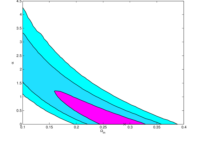
Constraints from SNeIa data on the CDM model are shown in Fig. 1. SNeIa data constrains the nonrelativistic matter density parameter to be less than 0.4 at about 3 confidence level. The parameter is constrained to be less than 4.5 at about 3 confidence level.
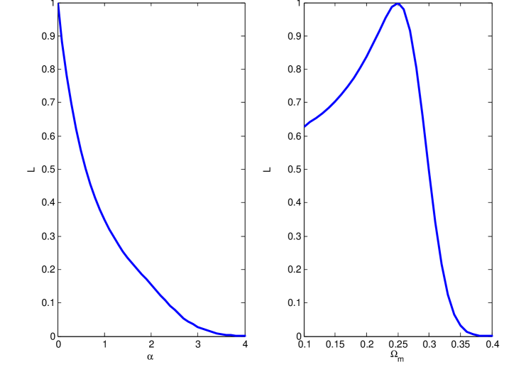
The one dimensional likelihood functions for individual cosmological parameters are shown in Fig. 2. The best fit values are and . The 1 intervals are and .
3 GRB as standard candles
One way of improving our understanding of how dark energy behaves is to study the evolution of the Universe at redshifts higher than those probed by SNeIa. This requires standard candles that are visible at greater distances. Gamma-ray bursts (GRBs) could in principle serve as such high redshift standardizable candles. They are the most luminous events in the Universe today and can be seen to beyond . If it is definitely established that GRBs are standardizable candles, their visibility at high redshift should prove to be very useful in discriminating between CDM and time-varying dark energy models.
With the intention of getting cosmological constraints from GRB observations a number of GRB calibrations have been used so far [95]. One that gives least scatter and therefore most information is
| (3) |
a relation that connects the total burst energy of the GRB () to the peak energy of the GRB spectrum () [96]. Regrettably, we do not yet have a model-independent way of computing the coefficients and . A better understanding of physical processes that result in the burst, or observations of nearby GRBs (to which distances can be measured independently), could in principle help us to calibrate the - relation without any prior assumptions. Until recently the only way to extract cosmological information from GRBs was to recalibrate them for every dark energy model considered (at each set of parameter values). This is time consuming and also results in large statistical uncertainties and hence GRB cosmological constraints that are poor.
Recently, two methods of calibrating GRBs in cosmology-independent manners have been proposed and used to constrain some dark energy models. One method externally calibrates GRBs, by using SNeIa measurements [97, 98, 99, 100], while the other uses GRB measurements alone [101]. While externally calibrating GRBs results in tighter cosmological constraints, internally calibrated GRB data may be straightforwardly combined with other data when deriving cosmological constraints. The resulting cosmological constraints are still loose, but in the future when more high precision GRB observations become available this could provide a strong test of dark energy.
Reference [101] recently used data of 69 GRBs [95] to construct a model-independent distance measure that can be used to constrain cosmological models. When this method is used to constrain CDM the GRB data favor lower values of both cosmological constant energy density () and nonrelativistic matter energy density () than do the SNeIa data. The GRB data by themself are unable to strongly constrain cosmological parameters, for example in spatially-flat CDM the GRB data require at 1 confidence [101].
4 Constraints from GRB data
Besides the - relation, Eq. (3), four other calibrations for GRBs are used in Ref. [101]. Reference [101] placed each of the 69 GRBs in the redshift range to at a luminosity distance that minimized a combined that took weighted account of all five calibration relations. From this [101] computed the cosmology-independent distance measure
| (4) |
where
| (5) |
and is the luminosity distance at redshift , and is the speed of light. The ratio in Eq. (4) does not depend on the Hubble constant and does not require information about the absolute calibration of GRBs (which are unknown).
Reference [101] computed the cosmology-independent distance measure in six redshift bins , . The values of are shown in Appendix 13 and the normalized covariance matrix is
| (6) |
For currently viable cosmological models, these are almost completely independent of the cosmological model and so provide a useful summary of current GRB data [101]. This information can be used to constrain any dark energy model and the resulting GRB data constraints can be straightforwardly combined with other constraints.
We compute the difference between the theoretical prediction and the measured value at each of the 6 redshifts,
| (7) |
and the function
| (8) |
where is the normalized covariance matrix given by Eq. (6) and summation over repeated indexes is assumed. Here is if and if , see Appendix 13.
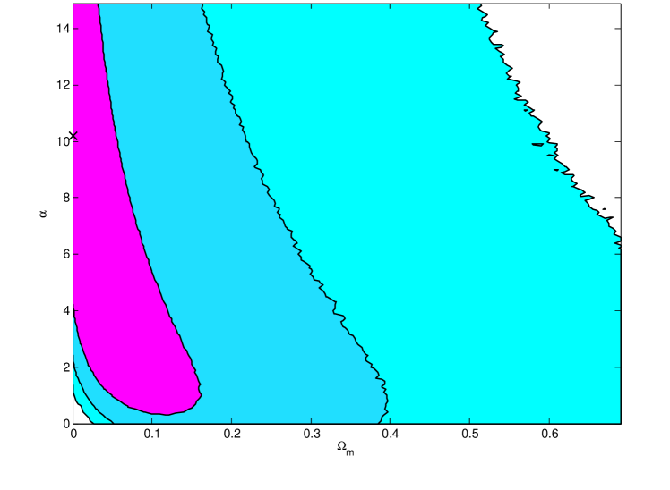
The constraints on CDM from GRB data are shown in Fig. 3. Current GRB data can not constrain cosmological parameters well and a wide range of values are at 3 confidence level. The best-fit parameter values are and with for 4 degrees of freedom.
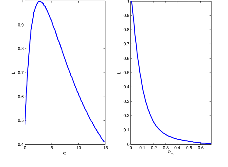
The one dimensional likelihood functions for individual parameters are shown in Fig. 4. The best fit parameter values are and . One standard deviation intervals are and .
GRB data by themselves do not provide tight constraints on cosmological parameters. Moreover, while not greatly significant, current GRB data favor cosmological parameter values that are at odds with what other data favor. When used in combination with some of the highest quality current data (e.g., SNeIa and BAO peak measurements) current GRB data only slightly change the results. This is mainly because in the absence of an absolute calibration of GRBs they, as standard candles, have big measurement uncertainties. This is however quite likely to change as more and better-quality GRB measurements become available and with improvements in how to calibrate GRBs. GRBs could potentially provide a very strong test of the time variation of dark energy as they can be observed up to redshifts beyond 8, at distances where other standard candles cannot be detected.
Chapter 6 Constraints from Cluster Gas Mass Fraction Data
This chapter is based on Ref. [111].
1 Using galaxy clusters as cosmological probes
Galaxy clusters are the biggest gravitationally bound objects in the Universe. Old, relaxed, rich ones should provide a fair sample of the matter content of the Universe. The ratio of baryonic mass to total nonrelativistic mass in the clusters should be close to the ratio of cosmological parameters , the baryonic fraction . More than of clusters’ baryonic mass is in hot X-ray emitting intergalactic gas. Estimates of gas mass fraction in clusters can be combined with the priors on from WMAP or BBN to get tight constrains on nonrelativistic matter density. During cosmic evolution the ratio should remain the same, but clusters are observed at different redshifts and since the reconstructed depends on the assumed distance to the cluster, this data can be used to constrain cosmic evolution and hence the dark energy.
To get a good estimate of , the gas mass fraction, large, relaxed clusters in thermal equilibrium should be used. Clusters with high core temperature () are better for the analysis, because in computer simulations and observations they have less systematic scatter in gas mass fraction compared to “cold” clusters.
The gas mass fraction is given by [6]
| (1) |
Here is a calibration constant that accounts for effects, such as accuracy of instrument calibration and X-ray modelling. A conservative Gaussian uncertainty is used in Ref. [6]. The factor accounts for the change in the angle subtended by the cluster between the reference cosmology and the cosmology of interest and is always very close to . models non-thermal pressure due to subsonic motion in the gas, cosmic rays, magnetic fields, etc. In the analysis of Ref. [6] uniform prior with is assumed. is the “bias” factor, the ratio by which the baryon fraction in the cluster differs from the same mean ratio in the Universe. The “bias” factor is modeled as [6] and cosmological simulations suggest the uniform priors and , [6]. The parameter models the baryon gas mass fraction in stars. We use the uniform prior with and the Gaussian prior with , [6]. is the angular diameter distance computed in a reference, spatially-flat CDM model with , and is the angular diameter distance computed in the CDM model.
2 Many dimensional integration
We use the modified technique discussed below to perform some of the integrals to account for these nuisance parameters, which have usually veen done numerically, as discussed next.
Let’s say we want to integrate a function on the interval . If this cannot be done analytically, different numerical integration algorithms may be used to compute the integral to a given precision.
If the problem is one dimensional and the integrand is reasonably well-behaved, can be subdivided into segments of equal length; in each segment can be interpolated by a polynomial; and the integral can be approximated by a sum [112]. The simplest method of this sort uses the trapezoidal Newton-Cotes formula
| (2) |
The error on the integral computed using Eq. (2) can be approximated by
| (3) |
where prime denotes the derivative. The error could be smaller than this if the function is sufficiently smooth.
This method can be applied to multi-dimensional integrals also, by transforming them into repeated one-dimensional integrals. The number of function evaluations required to get the same precision, however, will grow exponentially in this case and so will the required computational time. To sample a unit interval in one dimensional space with a distance between adjacent points of 0.01, only hundred evenly-spaced points are required. To do the same thing in 10 dimensional space will require points.
To cut down on computational time Monte-Carlo integration techniques can be employed. Monte-Carlo algorithms randomly pick points in the multi-dimensional space. By the law of large numbers, the error on an integral computed using Monte-Carlo method scales as independent of dimensionality.
The gas mass fraction in Eq. (1) depends on eight “nuisance” parameters. These are , , , , , , , and . To perform this eight-dimensional integration we use a method that in this particular case works faster than Monte-Carlo sampling.
Five out of eight nuisance parameters enter Eq. (1) as a redshift independent combination . We can think of each nuisance parameter as a random number with a given probability distribution function (PDF). Then will also be a random variable with some PDF.
We use the following statistics results [113]. If two random variables and are independent with PDFs and then variables , and are also random with PDFs
| (4) |
| (5) |
| (6) |
We first numerically compute the PDF for using Eqs. (4-6) and replace the the five-fold integration of the likelihood function by a one-dimensional integral. This reduces computational time significantly.
3 Constraints from data
We use the measurements of gas mass fraction of 42 hot, X-ray luminous, relaxed galaxy clusters in the redshift range of to [6]. The cluster gas mass fraction data is presented in Appendix 14. We integrate the likelihood over the Hubble constant with the Gaussian WMAP prior , and baryonic mass energy density with a Gaussian prior .
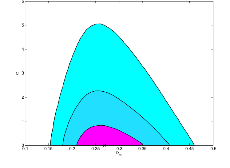
The constraints on CDM parameters are shown in Fig. 1. Brown, light blue and deep blue areas correspond to 1, 2, and 3 confidence levels respectively. The black cross denotes best-fit parameters and , with for 40 degrees of freedom. The nonrelativistic matter density is constrained to be in the range of at about 3 confidence level and is constrained to be less than 5 at about 3 confidence level.
One dimensional likelihood functions for individual parameters are shown in Fig. 2. The best-fit values from the one dimensional likelihood functions are and . 1 confidence level intervals from the one dimensional likelihood functions are and .
Chapter 7 Constraints on CDM from Baryon Acoustic Peak Measurements
1 Transverse baryon acoustic peak measurements
Before recombination baryons and photons are tightly coupled and gravity and pressure gradients induce sub-acoustic-Hubble-radius oscillations in the baryon-photon fluid [115, 116]. These transmute into the acoustic peaks observed now in the CMB anisotropy angular power spectrum, which provide very useful information on various cosmological parameters. The baryonic matter gravitationally interacts with the dark matter and so the matter power spectrum should also exhibit these “baryon acoustic” wiggles. Because the baryonic matter is a small fraction of the total matter the amplitudes of the BAO wiggles are small. The BAO peak length scale is set by the sound horizon at decoupling, , and so detecting the BAO peak in a real space correlation function requires observationally sampling a large volume. The BAO peak in the galaxy correlation function has recently been detected by using SDSS data [7, 117] and by using 2dFGRS data [118]. For more recent discussions of the observational situation see Refs. [119, 120, 8].
The sound horizon at decoupling can be computed from relatively well-measured quantities by using relatively well-established physics. Consequently it is a standard ruler and can be used to trace the universe’s expansion dynamics [121, 122, 123, 124]. A measurement of the BAO peak length scale at redshift fixes a combination of the angular diameter distance and Hubble parameter at that redshift. More precisely, what is determined [7] is the distance
| (1) |
where is the Hubble parameter and the angular diameter distance. depends on the cosmological parameters of the model, including those which describe dark energy, so we can constrain these parameters by comparing the predicted to the measurements.
We examine the constraints on CDM from two measurements of the BAO peak. The first is from the BAO peak measured at in the correlation function of luminous red galaxies in the SDSS [7]. This measurement results in (one standard deviation error), where the dimensionless and -independent function
| (2) |
and is the distance measure defined in Eq. (1). The measured value of does not depend on the dark energy model and only weakly depends on the baryonic energy density. The measurement also has a weak dependence on parameters like the spectral index of primordial scalar energy density perturbations (the assumed value is ) and the sum of the neutrino masses, but this is not strong enough to have significant effect on the final result. To constrain cosmological model parameters in this case we perform a standard analysis.
The second BAO peak measurement we use is from the correlation function of galaxy samples drawn from the SDSS and 2dFGRS at two different redshifts, and , as determined by Ref. [8]. This analysis includes the SDSS luminous red galaxies, so the the two BAO peak measurements are not statistically independent.
This measurement gives the correlated values and (one standard deviation errors), where is the comoving sound horizon at recombination. These two measurements are correlated, with the inverse of the correlation matrix given b
To compute we first compute the angular diameter distance to the surface of last scattering, . We then use the WMAP measurement of the apparent acoustic horizon angle in the CMB anisotropy data [125] to determine the sound horizon (where we ignore the WMAP measurement uncertainty and assume that is known perfectly). The use of the WMAP prior on the apparent acoustic horizon angle results in very tight constraints on the spatial curvature. When this measurement is not used, these measurements alone can not tightly constrain the dark energy parameters.
To constrain cosmological parameters in this case we follow Ref. [8] and first compute
| (3) |
where for definiteness we consider the CDM model. We then compute the function
| (4) |
and the likelihood function
| (5) |
2 Constraints from transverse BAO peak measuremnts
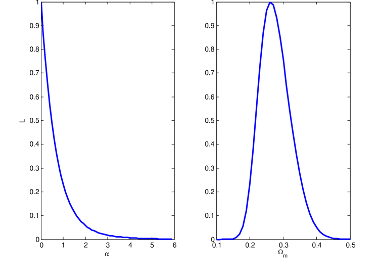
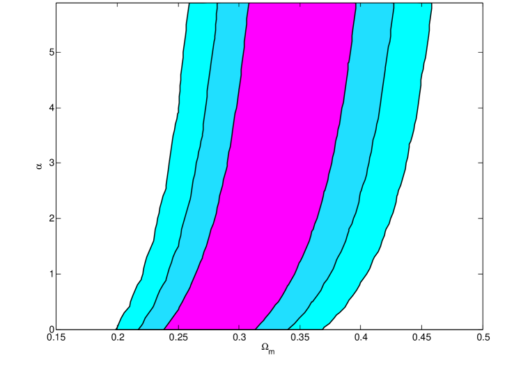
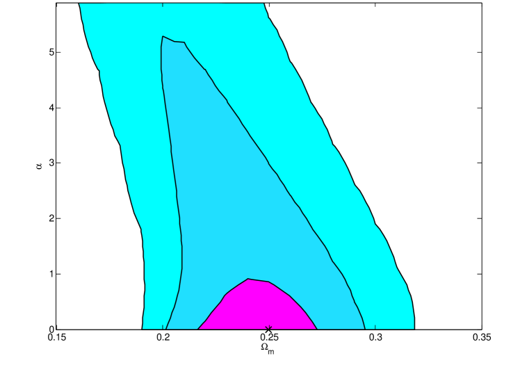
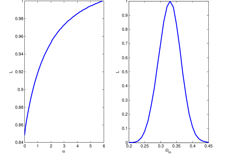
The constraints on CDM model from BAO data presented in Ref. [7] are shown in Fig. 1. Constrains from BAO data presented in Ref. [8] are shown in Fig. 2. The one dimensional individual likelihoods are shown in Figs. 3 and 4 respectively. The best fit values of individual parameters from Fig. 4 are and , with 1 intervals and .
These measurements were made at only two redshifts and by themselves do not provide a robust and reliable test of dark energy models, but in combination with other data they do provide useful constraints on cosmological parameters. In addition, a number of surveys are planned in next few years that will measure the BAO scale accurately and at a variety of redshifts up to . This upcoming BAO data, especially when combined with other data, will prove very useful in tightly constraining dark energy parameters [126].
3 Radial BAO peak measurements
Recently it was argued that the above measurements of the BAO scale were essentially measurements orthogonal to the line of sight and so statistically independent from a line of sight measurement of the BAO scale, even if the same galaxy catalog is used for both measurements. Reference [127] used the SDSS data to compute the line of sight or radial BAO scale in redshift space for two ranges of redshift and showed the resulting constraints on the spatially-flat XCDM parameterization [128]. These constraints from the radial BAO scale data are quite similar to the constraints derived from earlier “transverse” BAO scale measurements. The data are consistent with spatially-flat CDM. However, these current radial BAO measurements (like current non-radial BAO measurements) can not tightly constrain time-varying dark energy by themselves (although the situation is anticipated to improve in the next few years), as discussed next.
In a spherically symmetric Universe the two-point correlation function is a function of two variables, , where is the separation along the line of sight and is the separation on the sky. It can also be expressed as a function of absolute separation and the cosine of the angle between the line of sight and the direction of separation, . The correlation function can then be decomposed into multipole moments,
| (6) |
where is the order Legendre polynomial. Multipole moments of different orders can be related to each other if one has a complete theory of linear and nonlinear evolution. Although high multipoles that describe the “shape” of baryon acoustic oscillation imprints on the matter distribution are very difficult to measure in practice, theoretically they are independent of the monopole and could provide additional structure formation tests.
Initial work considered only the averaged over direction monopole part of the correlation function,
| (7) |
and found a BAO peak signal at a comoving distance of . This measurement was however mostly transverse to the line of sight direction ; the weight of separation along the line of sight contributes less then . Consequently, it is fair to assume that the radial baryon acoustic peak scale measurement in the line of sight direction from is statistically independent from that measured from , even if the same galaxy sample is used for both measurements.
Reference. [127] used SDSS data to measure the radial baryon acoustic scale in two redshift ranges with radial BAO peak scale and with (both one standard deviation errors). Theoretically the radial BAO peak scale is given by
| (8) |
where is the Hubble parameter at redshift , is the sound horizon size at the drag redshift , at which baryons were released from photons, and is the speed of light. can be easily computed in a given cosmological model and depends on model parameters such as the non-relativistic matter density and the time dependence of dark energy.
can be computed with two different methods. One is to use the ratio between the distance to the last-scattering surface and measured by CMB anisotropy experiments and compute the sound horizon at photon decoupling from
| (9) |
Here is the redshift at photon decoupling and is the angular diameter distance. Alternatively, one can use priors on the fractional energy density parameters of baryonic matter, , nonrelativistic matter, , and relativistic matter, , from, e.g., CMB anisotropy measurements, and compute the sound horizon at the drag redshift from
| (10) |
Both options have similar drawbacks. One has to assume priors on “nuisance” parameters like or various energy densities. CMB anisotropy measurements themselves have measurement errors that must be accounted for, otherwise the errors on the estimates of dark energy model parameters of interest will be underestimated. Also, the best fit values for nuisance parameters given by CMB anisotropy data are in general different for every cosmological model and also depend on model parameter values. To be fully consistent when using priors one would have to reanalyze CMB experiments for each cosmological model (and model parameter value) instead of using a single set of values for , , , and .
At present, however, the BAO scale is measured only in two redshift ranges and does not provide very tight parameter constraints compared to other observational tests. Hence, as long as we are interested in preliminary constraints on dark energy from BAO scale measurements we may use the simplified approach of Ref. [127], keeping in mind that when more and better quality BAO scale measurements become available a more complete, careful, and time-consuming analysis will be warranted.
4 Constraints from radial BAO peak measurements
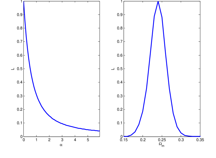
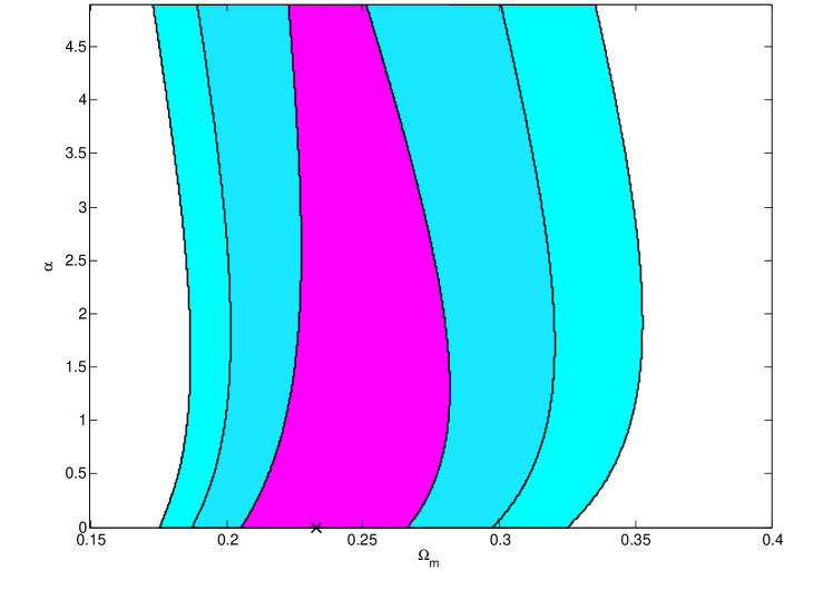
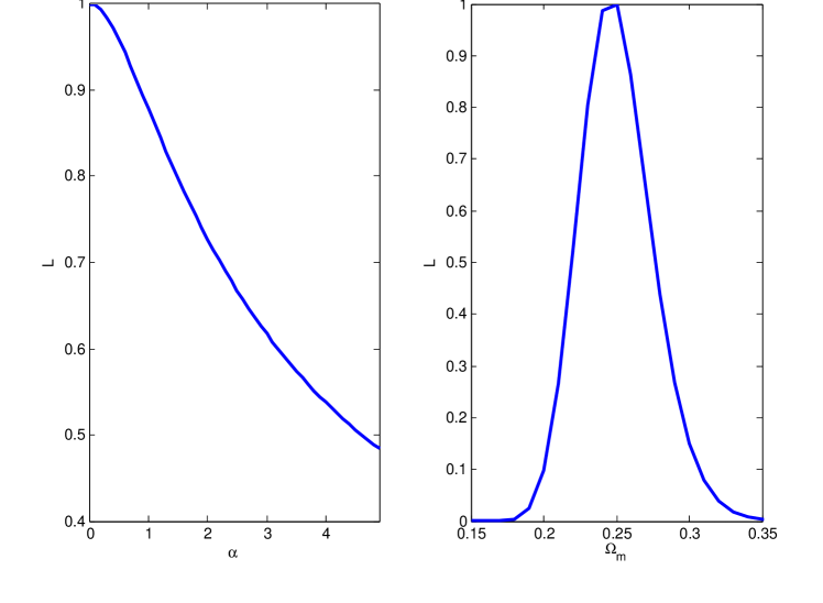
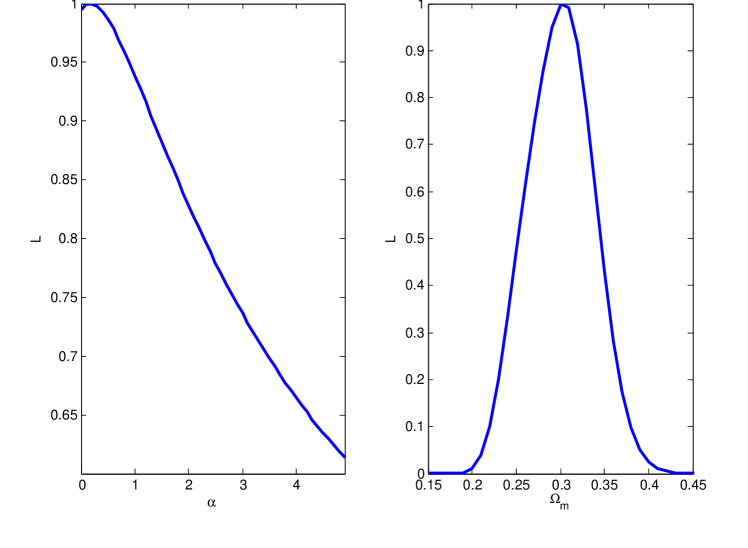
The confidence level contours for the spatially-flat CDM model are shown in Fig. 5 and 6. Corresponding one dimensional likelihood functions for individual cosmological parameters are shown in Fig. 7 and 8. Here, the radial BAO measurements constrain to be between and at about 3, but the parameter is not constrained well and large values of (relatively rapidly evolving dark energy) are not ruled out, although the likelihood peaks at . These results are similar to the ones derived earlier using the non-radial BAO peak scale measurements.
Chapter 8 Conclusion
1 Joint constraints
Chapters 4 to 7 present constraints on CDM model parameters using different available cosmological data sets. The lookback time versus redshift and the GRB data cannot at the moment constrain dark energy strongly. Likelihoods resulting from these two data sets are flat in the direction of and give preference to cosmological models with low nonrelativistic mass energy density , which is at odds with other observations, but this is not very significant.
In both cases this happens because the measurements are available only at a small number of redshifts (32 for lookback time data and 6 for GRB) and the measurement uncertainties are large. This should change when more and better quality data become available. In the future these two methods could prove to be very useful in constraining dark energy.
Constraints from SNeIa absolute magnitude versus redshift data, galaxy cluster gas mass fraction versus redshift data, and BAO peak measurements are considerably tighter. BAO peak measurements are not very effective in constraining the parameter at the moment, but they give very good constraints on nonrelativistic matter energy density. The power of the constraints seems surprising given that the BAO peak measurements have been made at only two redshifts so far. SNeIa and cluster gas mass fraction data are not that effective in constraining but provide upper limits on . Current data favors the time-independent cosmological constant, but there is a large part of time-evolving dark energy (CDM) parameter space that is still not ruled out.
Since none of the available data sets alone can simultaneously tightly constrain both cosmological parameters and , we derive tighter constraints by performing joint analyses of observational data. We get the best results when using SNeIa and BAO peak measurements; adding other data to the mix does not significantly improve the constraints. Since these two are independent we define the joint likelihood as the product of the individual likelihoods
| (1) |
The constraints derived from this joint likelihood function are shown in Fig. 1. The joint analyses results in much tighter constraints. The nonrelativistic matter density is in the range of and is constrained to be less than 1.5 at about 3 confidence. The best-fit values and correspond to slowly-varying dark energy but the time-independent cosmological constant also fits the data very well.
The likelihood functions of individual cosmological parameters are shown in Fig. 2. The best-fit values from one dimensional likelihood functions are and . The 1 intervals are and .
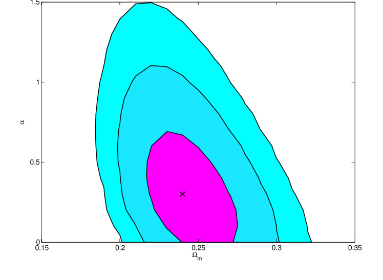
2 Future prospects of detecting time-evolving dark energy
Joint analysis of currently available cosmological data already results in strong constraints on the CDM model. is estimated to be in between 0.2 and 0.3 and is constrained to be less than 1.5.
The quality and quantity of available cosmological data sets is expected to increase significantly in the next decade. This will result in much tighter constraints on CDM model parameters. Some of the uncertainty in and comes from the fact that we do not know precise values of nuisance parameters, such as and . Ongoing surveys (such as HST) and new missions (such as PLANCK satellite) will measure these with greater accuracy, which will translate into better constraints on and .
From the joint analysis of near future SNeIa, GRB, galaxy cluster gas mass fraction and BAO measurements we should be able to either detect the time-dependence of dark energies energy density at a high confidence level or to constrain it to small, physically uninteresting values.
References
- [1] G. Hinshaw et al., Astrophys. J. Suppl. 180, 225 (2009).
- [2] D. W. Hogg et al., Astrophys. J. 624, 54 (2005).
- [3] M. Kowalski et al., Astrophys. J. 686, 749 (2008).
- [4] D. Rubin et al., Astrophys. J. 695, 391 (2009).
- [5] E. Komatsu et al., Astrophys. J. Suppl. 180, 330 (2009).
- [6] S. W. Allen et al., Mon. Not. Roy. Astron. Soc. 383, 879 (2008).
- [7] D. J. Eisenstein et al., Astrophys. J. 633, 560 (2005).
- [8] W. J. Percival et al., Mon. Not. Roy. Astron. Soc. 381, 1053 (2007).
- [9] W. J. Percival et al., Astrophys. J. 657, 645 (2007).
- [10] http://lambda.gsfc.nasa.gov.
- [11] P. J. E. Peebles, The large-scale structure of the universe, Princeton University Press, 1980.
- [12] P. J. E. Peebles, Physical Cosmology, Princeton University Press, 1994.
- [13] V. Mukhanov, Physical foundations of cosmology, Cambridge University Press, 2005.
- [14] S. Weinberg, Cosmology, Oxford University Press, 2008.
- [15] R. Durrer, The cosmic microwave background, Cambridge University Press, 2009.
- [16] A. G. Riess et al., Astron. J. 116, 1009 (1998).
- [17] S. Perlmutter et al., Astrophys. J. 553, 565 (1999).
- [18] R. A. Knop et al., Astrophys. J. 598, 102 (2003).
- [19] P. Astier et al., Astron. Astrophys. 447, 31 (2006).
- [20] G. Miknaitis et al., Astrophys. J. 666, 674 (2007).
- [21] N. Afshordi, Y.-S. Loh, and M. A. Strauss, Phys. Rev. D69, 083524 (2004).
- [22] S. P. Boughn and R. G. Crittenden, New Astron. Rev. 49, 75 (2005).
- [23] P. Fosalba, E. Gaztanaga, and F. Castander, Astrophys. J. 597, L89 (2003).
- [24] S. Weinberg, Rev. Mod. Phys. 61, 1 (1989).
- [25] L. Susskind, arXiv:hep-th/0302219 (2003).
- [26] R. Bousso and J. Polchinski, Sci. Am. 291, 60 (2004).
- [27] R. Watkins, H. A. Feldman, and M. J. Hudson, arXiv:0809.4041 (2008).
- [28] A. Kashlinsky, F. Atrio-Barandela, D. Kocevski, and H. Ebeling, Astrophys. J. 691, 1479 (2009).
- [29] A. Kashlinsky, F. Atrio-Barandela, D. Kocevski, and H. Ebeling, arXiv:0809.3734 (2008).
- [30] G. Lavaux, R. B. Tully, R. Mohayaee, and S. Colombi, arXiv:0810.3658 (2008).
- [31] A. Abate and P. Erdogdu, arXiv:0905.2967 (2009).
- [32] P. J. E. Peebles, Nuovo Cim. 122B, 1035 (2007).
- [33] H. Wei and S. N. Zhang, Phys. Rev. D78, 023011 (2008).
- [34] S. Tsujikawa and T. Tatekawa, Phys. Lett. B665, 325 (2008).
- [35] S. Capozziello, PoS QG-PH, 015 (2007).
- [36] T. P. Sotiriou and V. Faraoni, arXiv:0805.1726 (2008).
- [37] K. Bamba, S. Nojiri, and S. D. Odintsov, Phys. Rev. D77, 123532 (2008).
- [38] E. W. Kolb, S. Matarrese, and A. Riotto, New J. Phys. 8, 322 (2006).
- [39] C. M. Hirata and U. Seljak, Phys. Rev. D72, 083501 (2005).
- [40] S. Rasanen, Class. Quant. Grav. 23, 1823 (2006).
- [41] N. Li and D. J. Schwarz, Phys. Rev. D78, 083531 (2008).
- [42] P. J. E. Peebles and B. Ratra, Astrophys. J. 325, L17 (1988).
- [43] B. Ratra and P. J. E. Peebles, Phys. Rev. D37, 3406 (1988).
- [44] G. Olivares, F. Atrio-Barandela, and D. Pavon, Phys. Rev. D77, 063513 (2008).
- [45] H. Wei and S. N. Zhang, Phys. Rev. D76, 063003 (2007).
- [46] P. Wu and H. Yu, Astrophys. J. 658, 663 (2007).
- [47] S. A. Bonometto, L. Casarini, L. P. L. Colombo, and R. Mainini, arXiv:astro-ph/0612672 (2006).
- [48] B. Ratra and M. S. Vogeley, Publ. Astron. Soc. Pac. 120, 235 (2008).
- [49] E. V. Linder, Rept. Prog. Phys. 71, 056901 (2008).
- [50] J. Frieman, M. Turner, and D. Huterer, Ann. Rev. Astron. Astrophys. 46, 385 (2008).
- [51] J.-P. Uzan, Gen. Rel. Grav. 39, 307 (2007).
- [52] J. Frieman, C. T. Hill, A. Stebbins, and I. Waga, Phys. Rev. Lett. 75, 2077 (1995).
- [53] P. Brax and J. Martin, Phys. Lett. B 468, 40 (1999).
- [54] I. Zlatev, L. Wang, and P. J. Steinhardt, Phys. Rev. Lett. 82, 896 (1999).
- [55] V. Sahni and A. A. Starobinsky, Int. J. Mod. Phys. 9, 373 (2000).
- [56] A. Albrecht and C. Skordis, Phys. Rev. Lett. 84, 2076 (2000).
- [57] S. Podariu and B. Ratra, Astrophys. J. 563, 28 (2001).
- [58] S. Podariu, R. A. Daly, M. P. Mory, and B. Ratra, Astrophys. J. 584, 577 (2003).
- [59] G. Chen and B. Ratra, Astrophys. J. 582, 586 (2003).
- [60] G. Chen and B. Ratra, Astrophys. J. 612, L1 (2004).
- [61] K.-H. Chae, G. Chen, B. Ratra, and D.-W. Lee, Astrophys. J. 607, L71 (2004).
- [62] S. Podariu and B. Ratra, Astrophys. J. 532, 109 (2000).
- [63] S. Podariu, P. Nugent, and B. Ratra, Astrophys. J. 553, 39 (2001).
- [64] K. M. Wilson, G. Chen, and B. Ratra, Mod. Phys. Lett. A21, 2197 (2006).
- [65] P. J. E. Peebles and B. Ratra, Rev. Mod. Phys. 75, 559 (2003).
- [66] J. Martin, Mod. Phys. Lett. A23, 1252 (2008).
- [67] W. L. Freedman et al., Astrophys. J. 553, 47 (2001).
- [68] J. Dunkley et al., Astrophys. J. Suppl. 180, 306 (2009).
- [69] B. Fields and S. Sarkar, arXiv:astro-ph/0601514 (2006).
- [70] L. Samushia and B. Ratra, Astrophys. J. 650, L5 (2006).
- [71] L. Samushia, G. Chen, and B. Ratra, arXiv:0706.1963 (2007).
- [72] L. Samushia, A. Dev, D. Jain, and B. Ratra, ArXiv:0906.2734 (2009).
- [73] R. Jimenez and A. Loeb, Astrophys. J. 573, 37 (2002).
- [74] J. Simon, L. Verde, and R. Jimenez, Phys. Rev. D71, 123001 (2005).
- [75] R. G. Abraham et al., Astron. J. 127, 2455 (2004).
- [76] P. L. Nolan, W. F. Tompkins, I. A. Grenier, and P. F. Michelson, Astrophys. J. 597, 615 (2003).
- [77] T. Treu, M. Stiavelli, G. Bertin, S. Casertano, and P. Moller, Mon. Not. Roy. Astron. Soc. 326, 237 (2001).
- [78] T. Treu, M. Stiavelli, P. Moller, S. Casertano, and G. Bertin, Mon. Not. Roy. Astron. Soc. 326, 221 (2001).
- [79] H. Spinrad et al., arXiv:astro-ph/9702233 (1997).
- [80] J. Dunlop et al., Nature 381, 581 (1996).
- [81] R. Jimenez, private communications, 2009.
- [82] J. S. Alcaniz and J. A. S. Lima, Astrophys. J. 521, L87 (1999).
- [83] J. A. S. Lima and J. S. Alcaniz, Mon. Not. Roy. Astron. Soc. 317, 893 (2000).
- [84] D. Jain and A. Dev, Phys. Lett. B633, 436 (2006).
- [85] S. Capozziello, V. F. Cardone, M. Funaro, and S. Andreon, Phys. Rev. D70, 123501 (2004).
- [86] N. Pires, Z.-H. Zhu, and J. S. Alcaniz, Phys. Rev. D73, 123530 (2006).
- [87] M. A. Dantas, J. S. Alcaniz, D. Jain, and A. Dev, Astron. Astrophys. 467, 421 (2007).
- [88] M. A. Dantas and J. S. Alcaniz, arXiv:0901.2327 (2009).
- [89] Z.-L. Yi and T.-J. Zhang, Mod. Phys. Lett. A22, 41 (2007).
- [90] L. Samushia and B. Ratra, arXiv:0810.2104 (2008).
- [91] L. Samushia and B. Ratra, arXiv:0905.3836 (2009).
- [92] J. L. Tonry et al., Astrophys. J. 594, 1 (2003).
- [93] B. J. Barris et al., Astrophys. J. 602, 571 (2004).
- [94] A. G. Riess et al., Astrophys. J. 659, 98 (2007).
- [95] B. E. Schaefer, Astrophys. J. 660, 16 (2007).
- [96] G. Ghirlanda, G. Ghisellini, and D. Lazzati, Astrophys. J. 616, 331 (2004).
- [97] Y. Kodama et al., arXiv:0802.3428 (2008).
- [98] N. Liang, W. K. Xiao, Y. Liu, and S. N. Zhang, arXiv:0802.4262 (2008).
- [99] H. Wei and S. N. Zhang, arXiv:0808.2240 (2008).
- [100] N. Liang and S. N. Zhang, AIP Conf. Proc. 1065, 367 (2008).
- [101] Y. Wang, Phys. Rev. D78, 123532 (2008).
- [102] A. S. Friedman and J. S. Bloom, Nuovo Cim. 28C, 669 (2005).
- [103] C. Firmani, G. Ghisellini, G. Ghirlanda, and V. Avila-Reese, Mon. Not. Roy. Astron. Soc. 360, L1 (2005).
- [104] D. Xu, Z. Dai, and E. W. Liang, Astrophys. J. 633, 603 (2005).
- [105] E. Mortsell and J. Sollerman, JCAP 0506, 009 (2005).
- [106] H. J. Mosquera Cuesta, H. Dumet M., and C. Furlanetto, JCAP 0807, 004 (2008).
- [107] S. Basilakos and L. Perivolaropoulos, Mon. Not. Roy. Astron. Soc. 391, 411 (2008).
- [108] S. Capozziello and L. Izzo, arXiv:0806.1120 (2008).
- [109] R. Tsutsui et al., Mon. Not. Roy. Astron. Soc. Lett. 394, L31 (2009).
- [110] P. Meszaros, Rept. Prog. Phys. 69, 2259 (2006).
- [111] L. Samushia and B. Ratra, Astrophys. J. 680, L1 (2008).
- [112] W. H. Press et al., Numerical Recipes in C: The Art of Scientific Computing, Cambridge University Press, 1992.
- [113] K. F. Riley, M. P. Hibson, and S. J. Bense, Mathematical Methods of Physics and Engineering, Cambridge University Press, 2002.
- [114] L. Samushia and B. Ratra, arXiv:0806.2835 (2008).
- [115] R. A. Sunyaev and Y. B. Zeldovich, Astrophys. Space Sci. 7, 3 (1970).
- [116] P. J. E. Peebles and J. T. Yu, Astrophys. J. 162, 815 (1970).
- [117] G. Hutsi, arXiv:astro-ph/0507678 (2005).
- [118] S. Cole et al., Mon. Not. Roy. Astron. Soc. 362, 505 (2005).
- [119] N. Padmanabhan et al., Mon. Not. Roy. Astron. Soc. 378, 852 (2007).
- [120] W. J. Percival et al., Astrophys. J. 657, 51 (2007).
- [121] C. Blake and K. Glazebrook, Astrophys. J. 594, 665 (2003).
- [122] E. V. Linder, Phys. Rev. D68, 083504 (2003).
- [123] H.-J. Seo and D. J. Eisenstein, Astrophys. J. 598, 720 (2003).
- [124] W. Hu and Z. Haiman, Phys. Rev. D68, 063004 (2003).
- [125] D. N. Spergel et al., Astrophys. J. Suppl. 170, 377 (2007).
- [126] X. Wang et al., arXiv:0809.3002 (2008).
- [127] E. Gaztanaga, A. Cabre, and L. Hui, arXiv:0807.3551 (2008).
- [128] E. Gaztanaga, R. Miquel, and E. Sanchez, arXiv:0808.1921 (2008).
Chapter 9 C++ function for a numerical solution of the scalar field equations.
Chapter 10 Ages of passively evolving galaxies.
| Age (Gyr) | |
|---|---|
| 0.117100 | 10.2000 |
| 0.117400 | 10.0000 |
| 0.222000 | 9.00000 |
| 0.231100 | 9.00000 |
| 0.355900 | 7.60000 |
| 0.452000 | 6.80000 |
| 0.575000 | 7.00000 |
| 0.644000 | 6.00000 |
| 0.676000 | 6.00000 |
| 0.833000 | 6.00000 |
| 0.836000 | 5.80000 |
| 0.922000 | 5.50000 |
| 1.17900 | 4.60000 |
| 1.22200 | 3.50000 |
| 1.22400 | 4.30000 |
| 1.22500 | 3.50000 |
| 1.22600 | 3.50000 |
| 1.34000 | 3.40000 |
| 1.38000 | 3.50000 |
| 1.38300 | 3.50000 |
| 1.39600 | 3.60000 |
| 1.43000 | 3.20000 |
| 1.45000 | 3.20000 |
| 1.48800 | 3.00000 |
| 1.49000 | 3.60000 |
| 1.49300 | 3.20000 |
| 1.51000 | 2.80000 |
| 1.55000 | 3.00000 |
| 1.57600 | 2.50000 |
| 1.64200 | 3.00000 |
| 1.72500 | 2.60000 |
| 1.84500 | 2.50000 |
Chapter 11 Hubble parameter versus redshift data
| 0.09 | 69 | 12 |
| 0.17 | 83 | 8.3 |
| 0.27 | 70 | 14 |
| 0.4 | 87 | 17.4 |
| 0.88 | 117 | 23.4 |
| 1.3 | 168 | 13.4 |
| 1.43 | 177 | 14.2 |
| 1.53 | 140 | 14 |
| 1.75 | 202 | 40.4 |
Chapter 12 SNeIa “union” data set
| 0.050043 | 36.7730018543 | 0.153148680782 |
| 0.052926 | 36.8241423261 | 0.148454214927 |
| 0.02513 | 35.1678175291 | 0.165420933733 |
| 0.070086 | 37.567740156 | 0.15403068043 |
| 0.062668 | 37.5515804571 | 0.145317136417 |
| 0.087589 | 38.1915656352 | 0.159495013964 |
| 0.078577 | 37.5212710132 | 0.147429338762 |
| 0.017227 | 34.6546665523 | 0.1880259565 |
| 0.042233 | 36.3586532798 | 0.152312134352 |
| 0.045295 | 36.6566139461 | 0.148758275509 |
| 0.019599 | 34.5182384466 | 0.179081303451 |
| 0.100915 | 38.5088119689 | 0.145279087383 |
| 0.027342 | 35.2300574166 | 0.171939536277 |
| 0.074605 | 37.6663645268 | 0.147931348064 |
| 0.026489 | 35.5199700817 | 0.182864910719 |
| 0.049922 | 36.6999653546 | 0.146530609404 |
| 0.030604 | 35.5404531616 | 0.161624590233 |
| 0.016345641 | 34.0924538801 | 0.144775220876 |
| 0.0154363 | 34.0329851021 | 0.150597548663 |
| 0.030529 | 35.5818149937 | 0.0920067053122 |
| 0.024525 | 34.9577174302 | 0.109085696057 |
| 0.023953 | 34.935520479 | 0.115625212493 |
| 0.026038 | 35.3566237332 | 0.106784897071 |
| 0.048948 | 36.6391120177 | 0.1766982111 |
| 0.024314 | 35.0794913195 | 0.18643839963 |
| 0.015166 | 34.2041114924 | 0.225518080121 |
| 0.03572 | 36.1050539158 | 0.188094161827 |
| 0.048818 | 36.3507343053 | 0.166961986591 |
| 0.0219800059146 | 34.8811235819 | 0.196258768364 |
| 0.0275 | 35.6735856723 | 0.181507304221 |
| 0.1244 | 38.9521645786 | 0.168017789501 |
| 0.036 | 35.8260342723 | 0.173778570484 |
| 0.01673 | 34.1592687583 | 0.209352704395 |
| 0.016321 | 34.1144805357 | 0.209884301455 |
| 0.021793 | 34.9048499767 | 0.282608881266 |
| 0.01645 | 34.1818298266 | 0.292212075551 |
| 0.023208 | 35.117280195 | 0.276622195571 |
| 0.036457 | 36.1142750974 | 0.267250650207 |
| 0.019264 | 35.1559953619 | 0.285695464272 |
| 0.017605 | 34.3943547917 | 0.308882749558 |
| 0.031528 | 35.7346061594 | 0.270713039098 |
| 0.023536 | 35.1870287376 | 0.278885118559 |
| 0.016743 | 33.8878121745 | 0.292567467485 |
| 0.05371 | 36.4559044522 | 0.268351164818 |
| 0.016991 | 34.2677976869 | 0.290910806654 |
| 0.027865 | 35.0340198507 | 0.273008042132 |
| 0.017173 | 34.1860410198 | 0.293258906218 |
| 0.029955 | 35.9589514911 | 0.273866480307 |
| 0.016559 | 34.3764044862 | 0.292368203484 |
| 0.015 | 34.0959952821 | 0.145904476604 |
| 0.0544 | 36.9686138698 | 0.0771934613908 |
| 0.1561 | 39.294455039 | 0.0599663857105 |
| 0.0393 | 36.3055280023 | 0.0717497761757 |
| 0.1241 | 38.8100134766 | 0.0715971658275 |
| 0.1441 | 39.0528219919 | 0.0634435595707 |
| 0.1299 | 38.9956124177 | 0.0631822941145 |
| 0.0784 | 37.7810061412 | 0.0681153647931 |
| 0.62 | 43.2066240148 | 0.374321656282 |
| 0.57 | 42.6299495836 | 0.329397155099 |
| 0.3 | 40.9068557079 | 0.322661461524 |
| 0.38 | 41.981448045 | 0.294675002057 |
| 0.43 | 42.2865323661 | 0.353944288913 |
| 0.24 | 40.92039446 | 0.604691512396 |
| 0.3 | 40.152454556 | 0.463180764839 |
| 0.24 | 40.8941528415 | 0.281508606621 |
| 0.44 | 42.0189541221 | 0.290912412354 |
| 0.5 | 42.4251183643 | 0.285032220696 |
| 0.97 | 43.0841865629 | 0.742582169563 |
| 0.479 | 42.2593258058 | 0.305353355969 |
| 0.83 | 43.4934896902 | 0.372098016098 |
| 0.416 | 42.042208973 | 0.43961209764 |
| 0.581 | 41.9804788609 | 0.422581723678 |
| 0.45 | 41.7965293235 | 0.367900106831 |
| 0.579 | 43.1102730617 | 0.562403228541 |
| 0.32 | 41.1885505108 | 0.339690792497 |
| 0.657 | 43.0812935967 | 0.549444460563 |
| 0.472 | 42.0990717933 | 0.469994746225 |
| 0.374 | 43.1153409984 | 0.694417590782 |
| 0.526 | 42.013309316 | 0.402473462081 |
| 0.763 | 44.3657126034 | 0.885466302481 |
| 0.58 | 42.9398798711 | 0.395142768132 |
| 0.43 | 41.8899803061 | 0.393293335469 |
| 0.45 | 42.2825129374 | 0.422650328365 |
| 0.828 | 44.203018183 | 0.611918160502 |
| 0.656 | 43.181554143 | 0.528708119909 |
| 0.495 | 42.1205013485 | 0.39827409355 |
| 0.49 | 41.8217131258 | 0.355251221615 |
| 0.57 | 42.742574543 | 0.395438890913 |
| 0.388 | 42.0969738461 | 0.370734294336 |
| 0.45 | 42.2128189449 | 0.377256221564 |
| 0.48 | 42.1266258961 | 0.403490417945 |
| 0.615 | 42.6108744805 | 0.520864721236 |
| 0.4 | 42.1077687105 | 0.382043588034 |
| 0.655 | 42.3305104738 | 0.496246176513 |
| 0.498 | 43.0296153325 | 0.451179870261 |
| 0.465 | 41.8375675989 | 0.677740680801 |
| 0.453 | 42.6855854693 | 0.388547543287 |
| 0.425 | 41.3010835176 | 0.366453610612 |
| 0.278 | 40.6729770427 | 0.205733686158 |
| 0.477 | 42.0071669413 | 0.149503540949 |
| 0.95 | 43.6972613338 | 0.274437861244 |
| 1.057 | 44.0787405468 | 0.211584422417 |
| 0.816 | 43.7951226482 | 0.423980625959 |
| 0.455 | 42.3522141356 | 0.239111591348 |
| 0.514 | 42.4275455763 | 0.427580299971 |
| 0.423 | 41.6141933692 | 0.239548120652 |
| 0.946 | 43.1597477534 | 0.806741116211 |
| 0.859 | 44.022811801 | 0.304111603744 |
| 1.031 | 42.1761580597 | 1.28660173268 |
| 0.936 | 44.148887081 | 0.518330924179 |
| 0.528 | 42.3528772215 | 0.240748040733 |
| 0.645 | 44.0353749092 | 0.964152598465 |
| 0.978 | 43.6526492518 | 0.312966122482 |
| 0.885 | 44.1789952676 | 0.466461712419 |
| 0.815 | 44.1347089556 | 0.919484299622 |
| 0.568 | 42.5610152006 | 0.293309253351 |
| 0.711 | 43.2491247935 | 0.248908077637 |
| 0.3396 | 41.1022712766 | 0.259553392222 |
| 0.3965 | 41.4084095732 | 0.240552944224 |
| 0.812 | 43.8133209255 | 0.282936944717 |
| 0.799 | 43.1683351205 | 0.27444888856 |
| 0.882 | 42.9333230617 | 0.324847417172 |
| 0.833 | 43.407367536 | 0.347349605053 |
| 0.874 | 43.3865810553 | 0.462308366531 |
| 0.772 | 43.4354874701 | 0.263416996827 |
| 0.543 | 42.3919207564 | 0.135200439255 |
| 0.75 | 43.167266596 | 0.135523948437 |
| 0.64 | 42.7302552042 | 0.225082191179 |
| 0.43 | 42.202845059 | 0.143459564521 |
| 0.64 | 43.1881838551 | 0.186543501751 |
| 0.497 | 42.4090348089 | 0.158488764413 |
| 0.44 | 41.9964410659 | 0.127761277223 |
| 0.355 | 41.516716698 | 0.130966220782 |
| 0.78 | 43.4907628672 | 0.151115530925 |
| 0.54 | 42.4339111537 | 0.121366799166 |
| 0.86 | 43.7451019144 | 0.156150591229 |
| 1.02 | 44.1993977338 | 0.223075604603 |
| 1.14 | 44.2839104237 | 0.280516457089 |
| 0.854 | 43.9153676425 | 0.219112489318 |
| 1.37 | 44.7910462695 | 0.324513218653 |
| 0.975 | 44.2284945859 | 0.200606912017 |
| 0.97 | 44.5842379887 | 0.240421078134 |
| 0.74 | 43.417393486 | 0.196331774539 |
| 1.39 | 44.8274132597 | 0.591264643225 |
| 0.46 | 42.1615041182 | 0.190529350474 |
| 1.02 | 43.9810540565 | 0.241216980878 |
| 1.12 | 44.2495126581 | 0.241680223529 |
| 1.23 | 44.852264567 | 0.236250346674 |
| 1.19 | 44.1207308635 | 0.245756009721 |
| 0.839 | 43.5971981016 | 0.211771806558 |
| 1.01 | 44.4466207888 | 0.195202527359 |
| 0.521 | 42.4304300932 | 0.194708817687 |
| 0.475 | 42.1851461163 | 0.216179583718 |
| 0.95 | 43.7698442025 | 0.212959739832 |
| 1.3 | 44.9491044223 | 0.351060245309 |
| 1.305 | 44.4157049301 | 0.292031859582 |
| 0.526 | 43.0211775986 | 0.234516092908 |
| 0.735 | 43.1143549007 | 0.18304597653 |
| 1.14 | 44.0289616697 | 0.770661375912 |
| 1.551 | 45.3317386715 | 0.395907584039 |
| 1.265 | 44.6312640583 | 0.231966862578 |
| 1.34 | 44.953151304 | 0.252440440679 |
| 0.84 | 43.5620294075 | 0.195661579434 |
| 0.468 | 42.4934212383 | 0.156341752732 |
| 0.84 | 43.3513315259 | 0.326964462638 |
| 0.96 | 43.5868914421 | 0.427260522942 |
| 0.8218 | 43.5365504755 | 0.348162814934 |
| 0.93 | 44.6348635492 | 0.689119011672 |
| 0.451 | 41.8469440412 | 0.136544105548 |
| 0.61 | 42.8826976033 | 0.146106297403 |
| 0.83 | 44.6922378489 | 0.457964640542 |
| 0.707 | 43.320290922 | 0.250954794869 |
| 0.415 | 41.7696832434 | 0.12867036751 |
| 0.557 | 42.6475499276 | 0.146252717965 |
| 0.791 | 43.334857994 | 0.19213955201 |
| 0.695 | 43.1559541077 | 0.177154136049 |
| 0.633 | 43.200350196 | 0.204733134997 |
| 0.2486 | 40.6291787524 | 0.144170347426 |
| 0.532 | 42.6510205265 | 0.198544372744 |
| 0.331 | 40.9259072634 | 0.124868930577 |
| 0.346 | 41.2816358992 | 0.133990721793 |
| 0.961 | 44.0860127956 | 0.541232742301 |
| 0.613 | 42.9577096308 | 0.147055302427 |
| 0.3402 | 41.2627973103 | 0.124216129606 |
| 0.983 | 43.9686072633 | 0.873805060546 |
| 0.71 | 43.03031003 | 0.184976659207 |
| 0.73 | 43.3112856025 | 0.172061162401 |
| 0.47 | 42.2950363729 | 0.149449923436 |
| 0.62 | 43.0958537208 | 0.150521756378 |
| 0.521 | 42.2813323021 | 0.171703576261 |
| 0.369 | 41.5099445593 | 0.127128442179 |
| 0.571 | 42.4563923477 | 0.1847896727 |
| 0.604 | 42.4422921595 | 0.142594201708 |
| 0.9271 | 44.7438233798 | 0.616675765778 |
| 0.285 | 40.7117195315 | 0.128805577715 |
| 0.2912 | 40.7936031593 | 0.128325808339 |
| 0.548 | 42.684557193 | 0.163119668307 |
| 0.868 | 43.9551353049 | 0.697041426681 |
| 0.496 | 42.2194365099 | 0.160441226732 |
| 0.811 | 44.0557629679 | 0.356535950064 |
| 0.756 | 43.6720421887 | 0.2041097647 |
| 0.817 | 43.5678420781 | 0.305034089394 |
| 0.752 | 43.1434994817 | 0.179046394457 |
| 0.5516 | 42.4072918995 | 0.146846411569 |
| 0.3578 | 41.3894284101 | 0.125749074506 |
| 1.01 | 44.6896175735 | 0.910412577811 |
| 0.741 | 43.4820220235 | 0.161255047619 |
| 0.43 | 41.8372805299 | 0.138494545284 |
| 0.526 | 42.6736883867 | 0.151797295017 |
| 0.592 | 42.524194556 | 0.197075800472 |
| 0.905 | 43.686095579 | 0.424695030791 |
| 0.949 | 43.4679668471 | 0.467379485606 |
| 0.4607 | 41.9741739893 | 0.2613454679 |
| 0.3709 | 41.5023209499 | 0.132033007561 |
| 0.8 | 44.4199835555 | 0.537991937963 |
| 0.679 | 43.4170080051 | 0.175601683429 |
| 0.5817 | 42.8374976585 | 0.184185753799 |
| 0.55 | 42.3999711394 | 0.158230175273 |
| 0.81 | 43.7278491047 | 0.491922061811 |
| 0.95 | 43.780780395 | 0.421021094207 |
| 0.3373 | 41.1812895877 | 0.124867747916 |
| 0.91 | 44.4079361607 | 0.394461837584 |
| 0.263 | 40.6399477676 | 0.123324515918 |
| 0.643 | 43.0120301671 | 0.161285559543 |
| 0.691 | 43.1407175735 | 0.170861512594 |
| 0.357 | 41.3588695068 | 0.129068537648 |
| 0.721 | 43.1285593884 | 0.185537803758 |
| 0.581 | 42.7918076033 | 0.147505707094 |
| 0.6268 | 42.7073384153 | 0.145364365689 |
| 0.818 | 43.5731368588 | 0.562299153124 |
| 0.449 | 41.9045845939 | 0.150334954079 |
| 0.688 | 43.0446792667 | 0.179014967059 |
| 0.87 | 44.0828430243 | 0.496674095444 |
| 0.5043 | 42.3045856196 | 0.141778819311 |
| 0.591 | 43.3138714564 | 0.267379474385 |
| 0.426 | 41.806666569 | 0.204450457968 |
| 0.329 | 41.3757739861 | 0.25327455415 |
| 0.531 | 43.0629635087 | 0.301071564198 |
| 0.583 | 42.5993396847 | 0.461245287391 |
| 0.519 | 43.0898571036 | 0.385243880567 |
| 0.401 | 41.6214142647 | 0.259723821426 |
| 0.34 | 41.1002984666 | 0.22330741712 |
| 0.436 | 41.8355461879 | 0.219396208675 |
| 0.363 | 41.3991790454 | 0.206870861224 |
| 0.436 | 41.9186081822 | 0.214365467471 |
| 0.309 | 41.2854634774 | 0.20604264325 |
| 0.342 | 41.3335602868 | 0.20174070167 |
| 0.332 | 41.2428570494 | 0.223960203004 |
| 0.469 | 42.0869431125 | 0.219485296548 |
| 0.239 | 40.4663605358 | 0.193168326915 |
| 0.352 | 41.4402007529 | 0.222632458264 |
| 0.612 | 42.2601378946 | 0.819156755697 |
| 0.631 | 42.5665239435 | 0.270098723797 |
| 0.645 | 42.8315316986 | 0.22803549973 |
| 0.429 | 41.8321619796 | 0.217936090167 |
| 0.497 | 42.0900771628 | 0.23056454709 |
| 0.539 | 42.3621361424 | 0.235072095671 |
| 0.561 | 42.5988124145 | 0.254763512704 |
| 0.41 | 41.3480927299 | 0.217232818458 |
| 0.412 | 41.7758022341 | 0.2949457048 |
| 0.599 | 42.8544760765 | 0.290620357209 |
| 0.619 | 42.9246968389 | 0.246627072238 |
| 0.422 | 41.6678602675 | 0.238231296443 |
| 0.54 | 42.5656285356 | 0.254777678043 |
| 0.401 | 42.072813335 | 0.312075794951 |
| 0.218 | 40.3179435116 | 0.198433228858 |
| 0.633 | 42.2256486429 | 0.296301030677 |
| 0.383 | 41.592556266 | 0.228094106236 |
| 0.302 | 41.5660169963 | 0.259288152895 |
| 0.34 | 41.1438764437 | 0.199964450355 |
| 0.51 | 41.9188202391 | 0.258309489516 |
| 0.421 | 41.965762911 | 0.228780937104 |
| 0.399 | 41.7087506407 | 0.28376407894 |
| 0.493 | 42.122916001 | 0.229109806841 |
| 0.687 | 42.832217021 | 0.279368496827 |
| 0.502 | 41.8992528194 | 0.313490292477 |
| 0.687 | 42.8216812976 | 0.250279752764 |
| 0.495 | 42.2021639825 | 0.245006206755 |
| 0.603 | 42.6354160597 | 0.273892147864 |
| 0.421 | 42.0443812883 | 0.280749747008 |
| 0.348 | 41.5494690313 | 0.204875174321 |
| 0.213 | 40.3399930846 | 0.204646940237 |
| 0.344 | 41.0679683623 | 0.200210760141 |
| 0.271 | 40.5536369049 | 0.206465230307 |
| 0.564 | 42.3759756991 | 0.400947441397 |
| 0.274 | 40.7740469723 | 0.216212348503 |
| 0.582 | 43.2137150031 | 0.278992592748 |
| 0.68 | 42.8318958632 | 0.247902597912 |
| 0.401 | 41.9301329836 | 0.235368495661 |
| 0.416 | 41.7521888571 | 0.295167259169 |
| 0.286 | 41.387427719 | 0.334584228292 |
| 0.314 | 41.0209048393 | 0.287974294878 |
| 0.581 | 43.5994710152 | 0.377088903672 |
| 0.463 | 41.9546009246 | 0.265451577145 |
| 0.341 | 41.092049721 | 0.209704216095 |
| 0.671 | 42.1936025518 | 0.331542575911 |
| 0.631 | 42.9261055377 | 0.232187948068 |
| 0.522 | 42.6690298106 | 0.304891267733 |
| 0.368 | 41.4066563292 | 0.204741881488 |
| 0.309 | 40.8507297646 | 0.207725830155 |
| 0.528 | 42.4787440903 | 0.305372522825 |
| 0.268 | 40.7695452633 | 0.197555926698 |
| 0.695 | 42.9207400196 | 0.41358331096 |
| 0.284 | 40.7849823164 | 0.199874464698 |
| 0.508 | 42.1375516415 | 0.212951542267 |
| 0.781 | 43.3825529133 | 0.341139699918 |
| 0.613 | 42.4302887204 | 0.333098849656 |
Chapter 13 GRB data
| 0.17 | 1.0000 | ||
| 1.036 | 0.9416 | 0.1688 | 0.1710 |
| 1.902 | 1.0011 | 0.1395 | 0.1409 |
| 2.768 | 0.9604 | 0.1801 | 0.1785 |
| 3.634 | 1.0598 | 0.1907 | 0.1882 |
| 4.500 | 1.0163 | 0.2555 | 0.2559 |
| 6.600 | 1.0862 | 0.3339 | 0.3434 |
Chapter 14 Galaxy cluster gas mass fraction data set
| Cluster | ||
|---|---|---|
| Abell 1795 | 0.063 | |
| Abell 2029 | 0.078 | |
| Abell 478 | 0.088 | |
| PKS0745-191 | 0.103 | |
| Abell 1413 | 0.143 | |
| Abell 2204 | 0.152 | |
| Abell 383 | 0.188 | |
| Abell 963 | 0.206 | |
| RXJ0439.0+0521 | 0.208 | |
| RXJ1504.1-0248 | 0.215 | |
| Abell 2390 | 0.230 | |
| RXJ2129.6+0005 | 0.235 | |
| Abell 1835 | 0.252 | |
| Abell 611 | 0.288 | |
| Zwicky 3146 | 0.291 | |
| Abell 2537 | 0.295 | |
| MS2137.3-2353 | 0.313 | |
| MACSJ0242.6-2132 | 0.314 | |
| MACSJ1427.6-2521 | 0.318 | |
| MACSJ2229.8-2756 | 0.324 | |
| MACSJ0947.2+7623 | 0.345 | |
| MACSJ1931.8-2635 | 0.352 | |
| MACSJ1115.8+0129 | 0.355 | |
| MACSJ1532.9+3021 | 0.363 | |
| MACSJ0011.7-1523 | 0.378 | |
| MACSJ1720.3+3536 | 0.391 | |
| MACSJ0429.6-0253 | 0.399 | |
| MACSJ0159.8-0849 | 0.404 | |
| MACSJ2046.0-3430 | 0.423 | |
| MACSJ1359.2-1929 | 0.447 | |
| MACSJ0329.7-0212 | 0.450 | |
| RXJ1347.5-1144 | 0.451 | |
| 3C295 | 0.461 | |
| MACSJ1621.6+3810 | 0.461 | |
| MACS1427.3+4408 | 0.487 | |
| MACSJ1311.0-0311 | 0.494 | |
| MACSJ1423.8+2404 | 0.539 | |
| MACSJ0744.9+3927 | 0.686 | |
| MS1137.5+6625 | 0.782 | |
| ClJ1226.9+3332 | 0.892 | |
| CL1415.2+3612 | 1.028 | |
| 3C186 | 1.063 |