Theory and modeling of the magnetic field measurement in LISA PathFinder

Abstract

The magnetic diagnostics subsystem of the LISA Technology Package (LTP) on board the LISA PathFinder (LPF) spacecraft includes a set of four tri-axial fluxgate magnetometers, intended to measure with high precision the magnetic field at their respective positions. However, their readouts do not provide a direct measurement of the magnetic field at the positions of the test masses, and hence an interpolation method must be designed and implemented to obtain the values of the magnetic field at these positions. However, such interpolation process faces serious difficulties. Indeed, the size of the interpolation region is excessive for a linear interpolation to be reliable while, on the other hand, the number of magnetometer channels does not provide sufficient data to go beyond the linear approximation. We describe an alternative method to address this issue, by means of neural network algorithms. The key point in this approach is the ability of neural networks to learn from suitable training data representing the behavior of the magnetic field. Despite the relatively large distance between the test masses and the magnetometers, and the insufficient number of data channels, we find that our artificial neural network algorithm is able to reduce the estimation errors of the field and gradient down to levels below 10%, a quite satisfactory result. Learning efficiency can be best improved by making use of data obtained in on-ground measurements prior to mission launch in all relevant satellite locations and in real operation conditions. Reliable information on that appears to be essential for a meaningful assessment of magnetic noise in the LTP.

I Introduction

LISA Pathfinder (LPF) is a science and technology demonstrator programmed by the European Space Agency (ESA) within its LISA mission activities bib:LISA . LISA (Laser Interferometer Space Antenna) is a joint ESA-NASA mission which will be the first low frequency (milli-Hz) gravitational wave detector, and also the first space-borne gravitational wave observatory. LPF’s payload is the LISA Technology Package (LTP), and will be the highest sensitivity geodesic explorer flown to date. The LTP is designed to measure relative accelerations between two test masses (TM) in nominal free fall (geodesic motion) with a noise budget of

$$S^{1/2}_{\delta a,LPF}(\omega)\leq 3\times 10^{-14}\left[1+\left(\frac{\omega/2\pi}{3\;\rm{mHz}}\right)^{2}\right]\frac{\rm{m\;s}^{-2}}{\sqrt{\rm Hz}}$$ (1)

in the frequency band between 1 mHz and 30 mHz bib:trento .

Noise in the LTP arises as a consequence of various disturbances, mainly generated within the spacecraft itself, which limit the performance of the instrument. A number of these disturbances are monitored and dealt with by means of suitable devices, which form the so-called Diagnostics Subsystem bib:ere2006 . In LPF, this includes thermal and magnetic diagnostics, plus the radiation monitor, which provides counting and spectral information on ionizing particles hitting the spacecraft. The magnetic diagnostics system will be the subject of our attention here.

One of the most important functions of the LTP magnetic diagnostics is the determination of the magnetic field and its gradient at the positions of the TMs. For this, it includes a set of four tri-axial fluxgate magnetometers, intended to measure with high precision the magnetic field at the positions they occupy in the spacecraft — see figure 1. Their readouts do not however provide a direct measurement of the magnetic field at the positions where the TMs are, and an interpolation method must therefore be implemented to calculate it. In the circumstances we face, this is a difficult problem, mostly because the magnetometers layout is such that they are too distant from the locations of the TMs compared with the typical scales of the distribution of magnetic sources in the satellite. Its solution is however imperative since magnetic noise can be as high as 40 % of the total budget bib:trento given by Eq. (1), and hence it must be properly quantified.

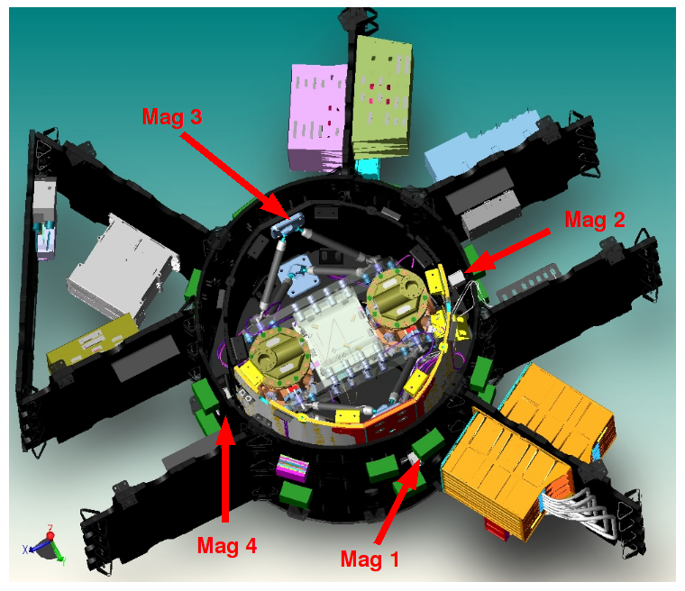
Figure 1: Artist view of the LPF science-craft. The LCA is in the center, surrounded by a double cylindrical shield. Outside it, a number of electronic boxes are represented, most of which are sources of magnetic field. The four magnetometers are the white little boxes indicated by the arrows (magnetometer #3 is however not visible), and are mounted on the outer cylindrical shell.

In order to design a suitable interpolation scheme, information on the actual distribution of magnetic sources is necessary. Data from the spacecraft manufacturer (EADS Astrium Stevenage, UK) have kindly been handed to us bib:wealthy for this purpose. According to these data, magnetic sources can be characterized as magnetic dipoles, whose positions are known and whose magnetic moments are only known in modulus — not in orientation. Most of these dipoles are associated to electronic boxes, with a few genuinely magnetic elements. An exception to this rule is the solar panels, which cover the entire spacecraft and can hardly be considered as a dipole as seen by the magnetometers. They are however designed so that their cells are arranged to minimize magnetic effects by having their rim wires wound contiguous and in opposite senses.

Astrium data are based on system design, so validation with the real spacecraft must be done by means of experiment, which is of course included in the planned activities before launch. Actually, though, the structure of the magnetic source distribution and their properties will not be directly visible either to the magnetometers or to the interpolation algorithms, which will just work with magnetic field values no matter how they are generated. Nevertheless, we think that the information available so far, though not final, qualifies very well as a guide to the elaboration of a magnetic model which will be needed to define and verify the performance of the analysis algorithms which will eventually be applied to the data delivered by the satellite in flight.

In this paper we will make use of the dipole model of the sources to assess the performance of two different types of interpolation methods: multipole interpolation and neural network algorithms. The first is the more immediate one to try, but as we will show below it is not as efficient as one might expect a priori. To overcome this problem we propose a novel method, based on neural networks. Based on the results obtained with the same dipole source model, our solution looks promising since the errors of the interpolated fields and gradients are significantly smaller than those obtained with the multipole approach. The paper is structured as follows. In Sect. II we provide a general description of the problem. It follows Sect. III, where we discuss the multipole interpolation, whereas in Sect. IV we explain our neural network approach. The results of applying this algorithm are presented in Sect. V, while in Sect. VI we summarize our major findings and we draw our conclusions.

II General description of the problem

Magnetic noise in the LTP is allowed to be a significant fraction of the total mission acceleration noise: $1.2\times 10^{-14}$ m s^-2 Hz^-1/2 can be apportioned to magnetism, i.e., 40 % of the total noise, 3$\times$10^-14 m s^-2 Hz^-1/2, see Eq. (1). This noise occurs because the residual magnetization and susceptibility of the TMs couple to the surrounding magnetic field, giving rise to a force

$${\bf F}=\left\langle\left[\left({\bf M}+\frac{\chi}{\mu_{0}}\,{\bf B}\right)\mbox{\boldmath${\cdot}\/$}\mbox{\boldmath${\nabla}\/$}\right]{\bf B}\right\rangle V$$ (2)

in each of the TMs. In this expression B is the magnetic field in the TM, $\chi$ and M are its magnetic susceptibility and density of magnetic moment (magnetization), respectively, and $V\/$ is the volume of the TM; $\mu_{0}$ is the vacuum magnetic constant, $4\pi\times 10^{-7}$ m kg s^-2 A^-2), and $\langle\cdots\rangle$ indicates TM volume average of the enclosed quantity. Moreover, the magnetic field and its gradient randomly fluctuate in the regions occupied by the test masses, thus resulting in a randomly fluctuating force:

$${\bf\delta F}=\left\langle\left[\left({\bf M}+\frac{\chi}{\mu_{0}}\,{\bf B}\right)\mbox{\boldmath${\cdot}\/$}\delta\mbox{\boldmath${\nabla}\/$}\right]{\bf B}+\frac{\chi}{\mu_{0}}\,\left[\delta{\bf B}\mbox{\boldmath${\cdot}\/$}\mbox{\boldmath${\nabla}\/$}\right]{\bf B}\right\rangle V$$ (3)

where $\delta{\bf B}$ represents the fluctuation of the magnetic field, and $\delta\mbox{\boldmath${\nabla}\/$}$ stands for the fluctuation of the gradient bib:ntcs .

Quantitative assessment of magnetic noise in the LTP clearly requires real-time monitoring of the magnetic field, which in LPF is done by means of a set of four tri-axial fluxgate magnetometers bib:DDS_LTP . These devices have a high-permeability magnetic core, which drives a design constraint to keep them somewhat far from the TMs. The price to be paid for this is that the measured field is not directly useful (we need to know it at the positions of the TMs). Hence, a procedure to estimate it at these positions, based on the data delivered by the magnetometers, must be set up.

As previously mentioned, the sources of magnetic field are essentially electronics boxes plus a few genuinely magnetic components inside the spacecraft. The interplanetary magnetic field is orders of magnitude weaker, hence of little relevance to the effects considered here, and solar panel effects will not be considered — see section I. There are no sources of magnetic field inside the LTP Core Assembly (LCA), all being placed outside its walls. The number of Astrium identified sources is around 40, and can be modeled as point magnetic dipoles bib:wealthy . Figure 2 gives an overview of the geometry, see caption for details.

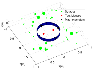
Figure 2: Conceptual diagram: magnetic sources (green dots, size proportional to the modulus of the magnetic moment of the source), Test Masses (red dots), and the four magnetometers (black triangles). Also represented (in dark blue) is the wall of the LCA.

III Multipole interpolation theory

Perhaps the most immediate (and obvious) procedure to interpolate the magnetic field is to resort to its multipole structure. This is known to be the best option in some mathematical sense bib:jackson . Consequently, we first describe the details of its implementation, and then we assess its practical merit.

We will treat the LCA region as a vacuum. This is a reasonable hypothesis, as the materials inside it are essentially non-magnetic. Accordingly, the magnetic field has zero divergence and rotational :

$$\mbox{\boldmath${\nabla}\/$}\mbox{\boldmath${\cdot}\/$}{\bf B}({\bf x},t)=0\quad\quad\mbox{\boldmath${\nabla}\/$}\times{\bf B}({\bf x},t)=0$$ (4)

Since $\mbox{\boldmath${\nabla}\/$}\times{\bf B}({\bf x},t)=0$, we thus have

$${\bf B}({\bf x},t)=\mbox{\boldmath${\nabla}\/$}\Psi({\bf x},t)$$ (5)

where $\Psi({\bf x},t)$ is a scalar function. Additionally, since $\mbox{\boldmath${\nabla}\/$}\mbox{\boldmath${\cdot}\/$}{\bf B}({\bf x},t)$ = 0, too, it immediately follows that $\Psi({\bf x},t)$ is a harmonic function, or

$$\nabla^{2}\Psi({\bf x},t)=0$$ (6)

The solution to this equation can be expressed as an orthogonal series of the form

$$\Psi({\bf x},t)=\sum_{l=0}^{\infty}\sum_{m=-l}^{l}\,M_{lm}(t)\,r^{l}\,Y_{lm}({\bf n})$$ (7)

where

$$r\equiv|{\bf x}|\ ,\qquad{\bf n}\equiv{\bf x}/r$$ (8)

are the spherical coordinates of the field point x, whose origin is by (arbitrary) convention assumed in the geometric center of the LCA. Equation (7) could also contain terms proportional to $r^{-l-1}$, but these have been dropped because the field cannot diverge at the center of the LCA. Actually, the expansion of Eq. (7) is only valid in a region interior to the closest field source. Finally, the coefficients $M_{lm}(t)$, which will be called multipole coefficients in the sequel, depend on the sources of magnetic field.

To obtain the field components we take the derivative of Eq. (7) following Eq. (5):

$${\bf B}({\bf x},t)=\mbox{\boldmath${\nabla}\/$}\Psi({\bf x},t)=\sum_{l=1}^{\infty}\sum_{m=-l}^{l}\,M_{lm}(t)\,\mbox{\boldmath${\nabla}\/$}[r^{l}\,Y_{lm}({\bf n})]$$ (9)

According to standard mathematics, the coefficients $M_{lm}(t)$ can be fully determined if the magnetic field is known at the boundary of the volume where the field equations are considered, in this case the LCA. This data is of course not available to us, since we only know B in four points of the boundary, where the magnetometers are. Therefore the question we need to address is: how many terms of the series can we possibly determine on the basis of the limited information available? Or, equivalently, how many multipole coefficients can we estimate, given the magnetometers readout data? Then, also, to which accuracy can we estimate the actual magnetic field after the maximum number of multipole coefficients have been calculated?

The answer to the first question above is actually not difficult: let us assume that the series in Eq. (9) is truncated after a maximum multipole index value $l\/$ = $L$. The estimated field, ${\bf B}_{\rm e}$, is then given by:

$${\bf B}_{\rm e}({\bf x},t)=\sum_{l=1}^{L}\sum_{m=-l}^{l}\,M_{lm}(t)\,\mbox{\boldmath${\nabla}\/$}[r^{l}\,Y_{lm}({\bf n})]$$ (10)

The number of terms in this sum is

$$N(L)=\sum_{l=1}^{L}\,(2l+1)=L(L+2)$$ (11)

which obviously equals the number of multipole coefficients needed to evaluate the sum. For example, we have $N(2)\/$ = 8 and $N(3)\/$ = 15. On the other hand, the number of magnetometer data channels is 12 — three channels per magnetometer, as the devices are tri-axial. This means we cannot push the series beyond the quadrupole ($l\/$ = 2) terms. This means that since we only have 12 data channels we have some redundancy to determine the first eight $M_{lm}(t)$ coefficients up to $l\/$ = 2, though we also lack information to evaluate the next seven octupole terms .

In order to make a best estimate of the $M_{lm}(t)$, a least-square method is set up as follows. Firstly, we define a quadratic error:

$$\varepsilon^{2}(M_{lm})=\sum_{s=1}^{4}\,\left|{\bf B}_{\rm r}({\bf x}_{s},t)-{\bf B}_{\rm e}({\bf x}_{s},t)\right|^{2}$$ (12)

where ${\bf B}_{\rm r}$ is the real magnetic field and the sum extends over the number of magnetometers, situated at positions ${\bf x}_{s}$ ($s\/$ = 1,…,4). We then find those values of $M_{lm}$ which minimize the error:

$$\frac{\partial\varepsilon^{2}}{\partial M_{lm}}=0$$ (13)

Once this system of equations is solved, the estimated coefficients $M_{lm}(t)$ are replaced back into Eq. (10) and then the spatial arguments x substituted by the positions of each test mass to finally obtain the interpolated field values. This process needs to be repeated for each instant $t\/$ of time at which measurements are taken, thereby generating the magnetic field time series. The gradient is estimated by taking the derivatives of Eq. (10):

$$\left.\frac{\partial B_{i}}{\partial x_{j}}\right|_{\rm e}({\bf x},t)=\sum_{l=0}^{L}\sum_{m=-l}^{l}\,M_{lm}(t)\;\frac{\partial^{2}}{\partial x_{i}\partial x_{j}}\left[r^{l}\,Y_{lm}({\bf n})\right]$$ (14)

It is to be noted that Eq. (10) is a polynomial of degree $L\/$$-$1 in the space coordinates $(x,y,z)$, hence its degree equals 1 when $L$ = 2. Since this is the most we can get of the magnetometer readout channels, the multipole expansion is actually equivalent to a linear interpolation of the field between its values at the boundary of the LCA and its interior. We may therefore not expect this method to produce excellent results, simply because the magnetic field inside the LCA is weaker than at its boundaries, the reason being that the magnetic field sources are outside the LCA. This valley structure of the magnetic field needs at least octupole (quadratic) terms to be approximated, but this would require at least one more vector magnetometer, which is not available. By the same argument, the field gradient can only be approximated by a constant value throughout the LCA — see Eq. (14).

III.1 Numerical simulations

In order to have a quantitative idea of the actual performance of the above interpolation scheme, we make use of the source dipole model. It has the following ingredients and assumptions:

1. The sources of magnetic are point dipoles outside the LCA.

2. The sources are those identified by Astrium Stevenage, as already mentioned, whose positions in the S/C are known. The set itself, as well as the source magnetic parameters need to be updated, but the data used (which date back to November 2006) qualifies to verify the performance of the interpolation methods.

3. The magnetic field created by the dipole distribution at a generic point x and time $t\/$ is therefore given by

   $${\bf B}({\bf x},t)=\frac{\mu_{0}}{4\pi}\;\sum_{a=1}^{n}\frac{3\left[{\bf m}_{a}(t)\mbox{\boldmath${\cdot}\/$}{\bf n}_{a}\right]\,{\bf n}_{a}-{\bf m}_{a}(t)}{\left|{\bf x}-{\bf x}_{a}\right|^{3}}$$ (15)

   where n_a =  $\left({\bf x}-{\bf x}_{a}\right)$/$\left|{\bf x}-{\bf x}_{a}\right|$ are unit vectors connecting the the $a$-th dipole m_a with the field point x, and $n\/$ is the number of dipoles.

4. Fluctuations of the dipoles, both in modulus and direction, are unknown, but this is not essential to assess the numerical performance of the algorithm.

We aim to compare interpolated magnetic field results with exact ones within the context and scope of the above model. To artificially simulate several possible scenarios, we will take advantage of the uncertainties in the source dipole orientations to randomly generate different magnetic field patterns, which we intend to reconstruct based on the multipole expansion. More specifically, the procedure is the following one:

1. Each dipole has a known fixed position in the spacecraft, and a fixed modulus, also known. The number of magnetic dipoles is also fixed to 37, which is the number in Astrium’s list.

2. The orientations of the dipoles are instead unknown. An example scenario is characterized by a specific selection of the 37 dipole orientations.

3. In order to explore the behavior of the algorithm, a batch of examples are examined, each corresponding to a randomly generated set of dipole orientations.

4. In each case, Eq. (13) is solved for $M_{lm}$, and the field estimate at each TM is then calculated with Eq. (10). In the last step, the result is compared with the theoretical one given in Eq. (15), and the differences annotated.

5. Finally, a statistical analysis of the differences (errors) is done.

The random character of the procedure may seem unrealistic, since the actual satellite configuration is not random. In this context, however, randomness is an efficient way of mimicking lack of knowledge. As we will see in the next section, numerical analysis based on this methodology sheds much light on the merits of the interpolation procedure — as it will also be the case when we come to neural networks performance in section V.

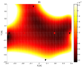
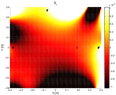
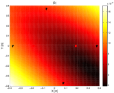
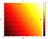
Figure 3: Magnetic field contour plots in the LCA region for a given source dipole configuration. $x\/$ is the direction between the two TMs, and $y\/$ is in the “horizontal” plane, which in the plot is at the TMs centres of mass altitude. Left panels: moduli of the magenetic field. The top panel displays the exact one, and the bottom one shows its multipole estimate. Right panels: same as in the left panels, but for one of the field components ($B_{x}$). The modulus of the magnetic field shows a complex structure in the central area, while $B_{x}\/$ has a saddle structure there — see along the diagonals of the frame graph. The red dots mark the centers of the TMs, and the black triangles the positions of the magnetometers.

III.1.1 Simulation results

In this section we summarise the most relevant results of the analysis of the multipole interpolation method. We use a batch of 1 000 example scenarios such as described above. Magnetic moment orientations were chosen by randomly picking values of the two defining spherical angles $(\theta,\varphi)$ from two independent uniform distributions.

Figure 3 graphically represents a magnetic field map in the LCA region corresponding to an arbitrarily chosen example out of the 1 000 considered. The valley structure is very clear in the $|{\bf B}|$ plot, while the $B_{x}\/$ component shows a saddle shape — see figure caption. $B_{y}\/$ and $B_{z}\/$ show qualitatively similar forms, and thus we do not show them. The elliptical forms in the estimate of $|{\bf B}|$ are due to the quadratic combination of the field components. The estimate of $B_{x}\/$ shows instead a linear structure, with constant gradient in all directions. Naked eye inspection immediately reveals a poor resemblance between estimated and exact quantities, but let us elaborate some numerical data.

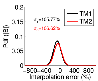
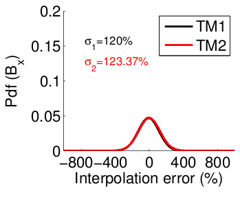
Figure 4: Binned errors of the estimated modulus of the magnetic field and of its $x\/$ component. They are reported in percentage. Colors correspond to each of the LTP TMs, respectively. Inset values of $\sigma$ indicate the rms half-width of the distributions. Solid lines are Gaussian fits to the histograms.

Figure 4 displays the binned distribution of estimation errors, defined by

$$\varepsilon(|{\bf B}|)=\frac{|{\bf B}_{\rm e}|-|{\bf B}_{\rm r}|}{|{\bf B}_{\rm r}|}\ ,\quad\varepsilon(B_{x})=\frac{B_{x,{\rm e}}-B_{x,{\rm r}}}{|{\bf B}_{\rm r}|}$$ (16)

where we have used a denominator $|{\bf B}_{\rm r}|$ in $\varepsilon(B_{x})$ to avoid meaningless infinities when $B_{x}\/$ is close to zero. $B_{y}\/$ and $B_{z}\/$ show similar trends and are not displayed. As can be seen, errors average to zero, but have rms deviations well above 100 %. Even worse, outliers are significant, as can be seen in Table 1, where averaged absolute values over the 1 000 simulated cases are displayed. Except, obviously, for the modulus error, we are around 500 %, but detailed examination of individual data further shows that errors as high as 2 000 % eventually happen.

Table 1: Averaged absolute value of the estimation errors in the components of the magnetic field and of its modulus. They are reported in relative percent.

	TM1	TM2
$\varepsilon(B_{x})$	493.7	640.4
$\varepsilon(B_{y})$	330.5	543.1
$\varepsilon(B_{z})$	359.5	368.2
$\varepsilon(|\bf{B}|)$	88.6	75.7

The most salient features of the numerical analysis can be briefly summarized. Firstly we find that magnetic field estimation errors are very variable, ranging from very few percent to over 1 000 % and, secondly, these huge uncertainties happen in an utterly random and fully unpredictable way. The a posteriori conclusion is quite simple: the intrinsic linear character of the interpolation scheme is not capable of reproducing the field structure inside the LCA — hence at the positions of the TMs — and, therefore, can produce very good or very bad results just by accident. In addition to not being predictable, the average error is any case too large. The ultimate reason for such poor performance is the the small number of magnetometers as well as their positioning: four magnetometers only allow for a field multipole expansion up to quadrupole terms, which means that the field values at the TMs are just linearly interpolated between magnetometer readouts at the boundary of the LCA. On the other hand, the magnetometers are closer to the magnetic field sources than they are to the TMs, which prevents resolution of the spatial field structure details inside the LCA with only linear terms in the space coordinates.

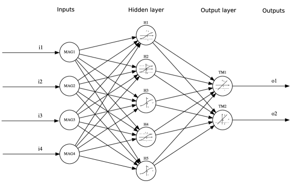
Figure 5: Feed-forward neural network architecture. Magnetometers readings are the system inputs, and estimates of the field and gradient at the positions of the test masses are the outputs of the system. In this architecture, only one intermediate, or hidden layer is assumed. Each of the circles represents one neuron and corresponds to the model of Eqs. (17) and (18).

IV A novel approach: neural networks

Search for an alternative approach to the above interpolation schemes is imperative, otherwise the information provided by the magnetometers will hardly be useful for the main goal of the LTP magnetic diagnostics system, i.e., to quantify the contribution of the magnetic noise to the total system noise. Here some promising results are presented on the implementation of a completely different methodology: neural networks bib:Kecman .

Artificial neural networks are made up of interconnecting artificial neurons (programming constructs that mimic the properties of biological neurons) that have the capacity to learn from processing data. Neural networks are often used in solving nonlinear classification and regression tasks by learning from data, hence are worth trying with the present problem bib:neuralPaper .

There are four sets of tasks which need to be implemented when solving a problem with artificial neural networks:

1. Neuron model selection

2. Model and architecture selection

3. Learning paradigm and learning algorithm selection

4. Performance assessment

We next go through them, one by one.

IV.1 Neuron model

The neuron is the basic unit of any neural network. It performs the following two operations:

• It collects the inputs from all other neurons connected to it and computes a weighted sum of the signals the latter inject into it, generally adding a bias as well. If we represent the inputs by a vector x $\equiv$ $(x_{1},\ldots,x_{n})$, and the weights by a w $\equiv$ $(x_{1},\ldots,w_{n})$ then this operation consists in calculating the sum

  $$\Sigma=w_{0}+\sum_{k=1}^{n}\,w_{k}x_{k}\equiv w_{0}+{\bf w}^{T}{\bf x}$$ (17)

  where the superindex $T\/$ stands for transpose matrix; in this case, w^T is a row vector while x is a column vector, so that ${\bf w}^{T}{\bf x}$ is the scalar product of w and x. A term $w_{0}$ is added to form the most general linear function of the vector argument x; it is called the bias.

• The above sum is used as the argument to the so-called activation function, $\varphi(\Sigma)$. The neuron’s output, also known as its activation, is thus

  $$o=\varphi(\Sigma)$$ (18)

  In general, $\varphi(\Sigma)$ can be selected in many different ways. Here, differentiable activation functions will be used, which suit well the gradient descent back-propagation learning algorithm — see sections below.

IV.2 Neural network architecture

Artificial neural networks are software or hardware models inspired by the structure and behavior of biological systems, and they are created by a set of neurons distributed in layers. There are many different types of neural networks in use today, but the architecture of a so-called feed-forward network, where each layer of neurons is linked with the next by means of a set of weights, is the most commonly used, and will also be used here. The specific architecture adopted in this study is shown in figure 5. The data streams coming from the magnetometers will be considered the system inputs, while magnetic field results and their gradients at the positions of the test masses will be the system outputs.

IV.3 Learning paradigms and learning/training algorithms

The investigation of learning algorithms is currently an active field of research. The design and implementation of an adequate training scheme is the essential ingredient for obtaining a good-quality estimate of the magnetic field and its gradient at the LTP TMs.

IV.3.1 Learning paradigms

There are two major learning paradigms, each corresponding to a particular abstract learning task. These are supervised learning and unsupervised learning.

1. Supervised learning. The idea of this paradigm is quite clearly suggested by its very name. A set of examples is filed, each set consisting in a number of vector of inputs (the magnetometers’ readouts in this case) and the corresponding values of the magnetic field and its gradient at the TMs for a given distribution of dipoles in the spacecraft. Let x represent a generic input vector, and y the associated vector output. These two vectors constitute an example. The set of filed examples for supervised learning is thus a set of pairs (x,y), where x$\in$$X\/$ and y$\in$$Y\/$, $X\/$ and $Y\/$ being some suitable sample spaces. The network is then fed the inputs x of one example and let it work out an output, o, say. This output is then compared with the correct one, y, and an error is calculated if o $\neq$ y. Iterations are then triggered to adjust the weighting factors such that the error is minimized. These will however vary as different examples are run, so a cost function is defined which enables the network to optimise the set of weights which works best for the set of examples analyzed, based on some suitable criterion.

2. Unsupervised learning. In unsupervised learning a cost function is to be minimized as well, but this function can be any relationship between x and the network output, o, but never taking into account the real expected target. The cost function is determined by the task formulation. Unsupervised learning is thus a form of self-adaptive system, whose guide is not an a priori knowledge of the final result but knowledge gained from experience.

In either case, the learning process is based on the architecture of the network, i.e., number of neurons and layers and their interconnections, as well as on the activation functions. These are parameters which, at least in the simplest cases, are tuned ab initio by the user based on observed performance of the network. In this study, supervised learning has been the implemented learning paradigm.

IV.3.2 Learning algorithms

There are many algorithms for training neural networks. When training feed-forward neural networks with supervised learning, a back-propagation algorithm is usually implemented. The error of the mapping at the output is propagated backwards in order to readjust the weights and improve the output error for the next iteration. The propagation can be implemented with different methods, the Ideal Gradient Descent being a classic which will also be used here, with slight modifications that make the algorithm convergence faster.

Iterations on the weights of the different neurons at the different layers proceed according to the following algorithm:

$${\bf w}_{n+1}={\bf w}_{n}-\eta\left.\frac{\partial E}{\partial{\bf w}}\right|_{n}$$ (19)

where $n\/$ labels the current iteration step, and $\eta\/$ is the learning rate, adjustable by the user. $E\/$ is the sum over the set of training examples of the square errors of the outputs:

$$E=\sum_{s}\;({\bf o}-{\bf y})^{T}\,({\bf o}-{\bf y})$$ (20)

where $s\/$ stands for the number of examples, o is the (vector) output from the network, while y is the target, or correct output in the corresponding example. The quantity $E\/$ can only be defined in supervised learning, of course, and the idea of the above procedure is to find that point in weight space where $E\/$ is an absolute minimum. $E\/$ can therefore be considered the cost function to be minimized in this particular supervised training scheme, also known as batch mode as the analysis is done across the entire set of training patterns in a single block.

There are a number of technical issues in pursuing the iterations in Eq. (19), such as the choice of the initial set of weights, the identification of local minima of $E\/$, the boundary effects,…which need to be addressed in each specific case. We skip a detailed discussion of these matters here and we focus on the results obtained using our method. For further details, the reader is referred to Refs. bib:Kecman and bib:neuralPrunning .

IV.4 Performance assessment

In this last step, the trained network must be tested with examples which differ from those used in the learning process. This is needed to assess whether or not the trained neural network is able to generate the expected results when fed with previously unseen inputs, hence determine its usability for the specific purpose it is intended.

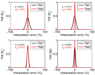
Figure 6: Error distributions for each field component at the position of test mass 1 (black line) and test mass 2 (red line). The top left panel displays the results for $B_{x}$, the top right panel shows the error distribution for $B_{y}$, while the bottom left panel depicts the distribution obtained for $B_{z}$ and the bottom right panel that for $|{\bf B}|$.

V Results

Training and testing have been done based on different field realizations, using the same model of sources and magnetic field described in section III.1, i.e., each example will consist in the magnetic field at the magnetometers’ positions, plus the magnetic field and gradient at the TM positions, all of them corresponding to a given configuration of the 37 Astrium dipoles.

Two different batches of examples, each including 1 000 realizations of a possible magnetic environment, have been generated following the directives explained in section III.1. The first batch has been used as the training set for a neural network with 12 inputs (3 inputs for each of the 4 vector magnetometers) and 16 outputs representing the field information at the position of the two test masses (3 field plus 5 gradient components per test mass ). The second batch has been used for validation to assess the performance of the network in front of unseen magnetometers readings.

V.1 Field estimation

Figure 6 shows the distribution of relative errors (in percentage) of the estimated components of the magnetic field at the positions of each TM. The plot is based on the results of the 1 000 validation runs described in the previous section. As can be observed, the order of magnitude of the errors of the estimated fields are now within much more acceptable margins (below $\sim 15\%$). This represents a reduction of estimation errors of more than one order of magnitude in comparison with the multipole expansion method.

During the training process, the neural network eventually learns that the magnetic field at the TMs is generally smaller than the magnetometers read — with occasional exceptions due to the rich and complex structure of the field inside the LCA, see e.g. figure 3. The neural network is able to derive an inference procedure which is actually quite efficient, and it does so by proper adjustment of its weight matrix coefficients w as explained in section IV.3.1. In order to better understand the reaction of the trained neural network to the magnetometers’ data, we found instructive and expedient to look into relationships between the data read by the magnetometers and the magnetic field estimates generated at the output of the neural network. We chose to calculate correlation coefficients between input and output data, and the results are displayed in Figure 7. The following major features are identified:

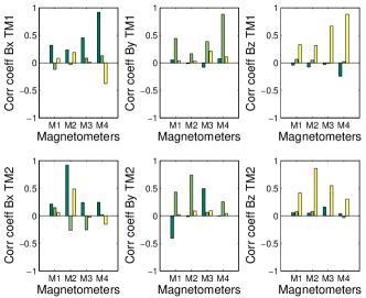
Figure 7: Correlation coefficient between the information entering the network (each magnetometer input) and the outputs provided by the trained network for the field estimates.

• Each component of the field is basically estimated from the magnetometers reading of the same component. For example, the interpolation of the $B_{x}\/$ component in test mass 1 is mostly dependent on the $B_{x}\/$ readings of the magnetometers.

• The measurements of the magnetometers closer to the interpolation points have larger weights. For instance, when the field is estimated at the position of TM1, to which M4 is the closest magnetometer, the value it measures is the largest contributor to the interpolated field in TM1. At the same time, M1 and M3 being nearly equidistant from both test masses, their weights are almost identical.

V.2 Gradient interpolation

The magnetic field gradient can also be estimated. The 9 components $\partial B_{i}/\partial B_{j}$ of the gradient are not independent, since they must verify Eqs. (4), which reduce their number to 5. The remaining 4 components can be easily calculated thereafter. Another option is to estimate the 9 gradient components regardless of the previously mentioned constraint, in which case they are actually found not to satisfy them. Discrepancies are however within the estimation error range, so we do not adopt this option here as it is slightly more cumbersome due to the correspondingly increased complexity of the network.

Results on gradient estimation are shown in Figure 8 for $\mbox{\boldmath${\nabla}\/$}B_{x}$ at the positions of both TMs. As can be observed, they are also within much more acceptable margins than the earlier interpolation approach could possibly produce. It is to be noted that no apparent or easily deductible physical relationship is found between the estimated gradient at the test mass positions and the magnetometer inputs, in contrast with what we have found for the field estimation.

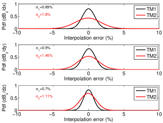
Figure 8: Probability density function of the errors distribution for the three components of $\mbox{\boldmath${\nabla}\/$}B_{x}$. From top to bottom: $\partial B_{x}/\partial x$, $\partial B_{x}/\partial y$ and $\partial B_{x}/\partial z$ at the positions of the test masses. Errors are given in percentages, the black lines corresponding to TM1, and the red ones to TM2.

V.3 Statistical analysis

Table 2: Statistical properties of the distribution of errors of the interpolated magnetic field.

	$\sigma$	$\gamma_{1}$	$\gamma_{2}$
	Multipole interpolation
$B_{x}$(TM1)	130.7583	-0.2782	19.3869
$B_{x}$(TM2)	128.3601	-0.1009	21.4974
$|\bf{B}|$(TM1)	105.5386	-3.6770	29.7343
$|\bf{B}|$(TM2)	102.1037	-4.4770	38.0686
	Neural network interpolation
$B_{x}$(TM1)	1.5204	-0.0028	2.7746
$B_{x}$(TM2)	1.6260	-0.0008	2.8626
$|\bf{B}|$(TM1)	1.4464	-0.1014	2.9440
$|\bf{B}|$(TM2)	1.3682	-0.0969	2.9905

In Table 2 we present a statistical comparison of the properties of the distribution of interpolated magnetic fields. For the sake of conciseness we only list the statistical properties of the interpolated modulus and $x$-component of the magnetic field. In particular, we show the standard deviation ($\sigma$) of the interpolating errors for both the multipole interpolation and the neural network estimate, the skewness of the distribution ($\gamma_{1}$) and the corresponding kurtosis ($\gamma_{2}$). Clearly, and as already mentioned, the interpolating errors are very large for the case in which a multipole interpolating scheme is used, as clearly shown by the very large standard deviation obtained when using this method. Also interesting to note is that for the case of the $x$-component of the magnetic field both methods yield distributions which are almost symmetrical. However this is not the case for the modulus of the magnetic field when the multipole interpolating method is used. Finally, the kurtosis of the multipole interpolation is very large, revealing a large number of outliers. All in all, a look at Table 2 reveals that the neural network method presents much better statistical properties than the multipole interpolation.

VI Conclusions

The magnetic diagnostics sensor set in the LTP is such that to infer the magnetic field and gradient at the positions of the TMs based on the readouts of the magnetometers is far from simple. The more standard interpolation scheme, based on a multipole expansion of the magnetic field inside the LCA volume, cannot go beyond quadrupole order which, in practice, means that just a linear approximation can be done, due to the reduced number of magnetometers available. This grossly fails to produce reliable results, with errors exceedingly large. This has motivated our search for better alternatives. Artificial neural networks have been presented as a more elaborate, non-linear procedure to estimate the required field values at the TM positions. In this paper we have presented results which very significantly improve the performance of the multipole expansion technique by almost two orders of magnitude. This a very encouraging outcome which points to the use of the neural networks as the baseline tool to analyse LTP magnetic data.

One of the main problems of using the neural network to assess the magnetic field at the positions of the test masses is to find a training process adequate to the set of data that the magnetometers will deliver in flight. This underlines the need to characterize on ground to our best ability the magnetic field distribution across the LCA for as many as possible foreseeable working conditions, both regarding DC and fluctuating values. Reliable information on this is essential for a meaningful assessment of magnetic noise in the LTP. However, the neural network analyses presented in this paper only apply to static fields. What they actually show is that neural networks work very well ($\sim$ 10 % accuracies) no matter which the source dipole configuration is. A different issue, which is beyond the scope of this paper and it is currently under investigation, is how to deal with time series of magnetometer readouts, which is of course the kind of data the satellite will transmit to ground. Features such as trends, field fluctuations,…will likely happen during mission operations, and the neural network algorithm must be trained to properly deal with them. Preliminary results indicate that the network is able to deal with moderate trends and levels of fluctuations, but further effort is needed to explore alternatives, e.g. self-adaptability, which will make more robust the performance of the system.

- (1) The LISA International Team 2008 ESA-NASA Report LISA-SCRD-Iss5-Rev1 (2008).
- (2) S Vitale Science Requirements and Top-level Architecture Definition for the Lisa Technology Package (LTP) on Board LISA Pathfinder (SMART-2), Report no. LTPA-UTN-ScRD-Iss003-Rev1 (2005).
- (3) Araújo H et al. J. of Phys. Conf. Ser. 66, 012003 (2007).
- (4) Private communication from David Wealthy (Astrium Stevenage, UK).
- (5) J. Sanjuán et al. Rev. of Sci. Inst. 79 084503 (2008).
- (6) P Canizares et al. Class. & Quantum Grav. 26, 094005 (2009).
- (7) J D Jackson, Classical Electrodynamics John Wiley & Sons, 3rd edition (1999)
- (8) V Kecman Learning and soft computing The MIT Press, 1st edition (2001).
- (9) C Serpico and C Visone IEEE Trans. on Magnetics, 34 623-628 (1998).
- (10) R Reed Prunning algorithms — A survey IEEE Trans. on Neural Networks, 4 740-747 (1993).