Abstract

In this paper the asymptotic behavior of an unstable integer-valued autoregressive model of order $p$ (INAR($p$)) is described. Under a natural assumption it is proved that the sequence of appropriately scaled random step functions formed from an unstable INAR($p$) process converges weakly towards a squared Bessel process. We note that this limit behavior is quite different from that of familiar unstable autoregressive processes of order $p$. An application for Boston armed robberies data set is presented.

1 Introduction

Recently, there has been remarkable interest in integer-valued time series models and a number of results are now available in specialized monographs (e.g., MacDonald and Zucchini [47], Cameron and Trivedi [12], and Steutel and van Harn [64]) and review papers (e.g., McKenzie [51], Jung and Tremayne [37], and Weiß [68]). Reasons to introduce discrete data models come from the need to account for the discrete nature of certain data sets, often counts of events, objects or individuals. Examples of applications can be found in the analysis of time series of count data on the area of financial mathematics by analyzing stock transactions (Quoreshi [57]), insurance by modeling claim counts (Gouriéroux and Jasiak [26]), medicine by investigating disease incidence (Cardinal et al. [13]), neurobiology by change-point analysis of neuron spike train data (Bélisle et al. [4]), optimal alarm systems (Monteiro et al. [52]), psychometrics by treating longitudinal count data (Böckenholt [7], [8]), environmetrics by analyzing rainfall measurements (Thyregod et al. [65]), experimental biology (Zhou and Basawa [69]), and queueing systems (Ahn et al. [1] and Pickands III and Stine [56]).

Among the most successful integer-valued time series models proposed in the literature we mention the INteger-valued AutoRegressive model of order $p$  (INAR($p$)). This model was first introduced by McKenzie [50] and Al-Osh and Alzaid [2] for the case $p=1$. The INAR(1) model has been investigated by several authors. Franke and Seligmann [22] analyzed maximum likelihood estimation of parameters under Poisson innovation. Du and Li [19] and Freeland and McCabe [24] derived the limit-distribution of the conditional least squares estimator of the autoregressive parameter. Silva and Oliveira [60] proposed a frequency domain based estimator, Brännäs and Hellström [9] investigated generalized method of moment estimation, Silva and Silva [62] considered a Yule-Walker estimator. Jung et al. [36] analyzed the finite sample behavior of several estimators by a Monte Carlo study. Ispány et al. [31], [32] derived asymptotic inference for nearly unstable INAR(1) models which has been refined by Drost et al. [17] later. A Poisson limit theorem has been proved for an inhomogeneous nearly critical INAR(1) model by Györfi et al. [27].

The more general INAR($p$) processes were first introduced by Al-Osh and Alzaid [3]. In their setup the autocorrelation structure of the process corresponds to that of an ARMA($p,p-1$) process, see also Section 2. Another definition of an INAR(p) process was proposed independently by Du and Li [19] and by Gauthier and Latour [25] and Latour [44], and is different from that of Alzaid and Al-Osh [3]. In Du and Li’s setup the autocorrelation structure of an INAR($p$) process is the same as that of an AR($p$) process. The setup of Du and Li [19] has been followed by most of the authors, and our approach will also be the same, see Section 2. The INAR($p$) model has been investigated by several authors from different points of views. Drost et al. [16] provided asymptotically efficient estimator for the parameters. Silva and Oliveira [61] described the higher order moments and cumulants of INAR($p$) processes, and Silva and Silva [62] derived asymptotic distribution of the Yule-Walker estimator. Drost et al. [18] considered semiparametric INAR($p$) models and proposed efficient estimation for the autoregression parameters and innovation distributions. Recently, the so called $p$-order Rounded INteger-valued AutoRegressive (RINAR($p$)) time series model was introduced and studied by Kachour and Yao [39] and Kachour [38]. The broad scope of the empirical literature in which INAR models are applied indicates its relevance. Examples of such applications include Franke and Seligmann [22] (epileptic seizure counts), Böckenholt [8] (longitudional count data), Thyregod et al. [65] (rainfall measurements), Brännäs and Hellström [9] and Rudholm [59] (economics), Brännäs and Shahiduzzaman [10] (finance), Gourieroux and Jasiak [26] (insurance), Pavlopoulos and Karlis [54] (environmental studies) and McCabe et al. [49] (finance and mortality).

An interesting problem, which has not yet been addressed for INAR($p$) models, is to investigate the asymptotic behavior of unstable INAR($p$) processes, i.e., when the characteristic polynomial has a unit root. In this paper we give a complete description of this limit behavior. In particular, it will turn out that an INAR($p$) model is unstable if and only if the sum of its autoregressive parameters equals 1, and in this case the only unit root of the characteristic polynomial is 1 with multiplicity one. For the sake of convenience, we suppose that the process starts from zero. Without loss of generality, we may suppose that the $p$th autoregressive parameter is strictly positive and that the greatest common divisor of the strictly positive autoregressive parameters is 1, see Remark 2.2. Under the assumption that the second moment of the innovation distribution is finite, we prove that the sequence of appropriately scaled random step functions formed from an unstable INAR($p$) process converges weakly towards a squared Bessel process. This limit process is a continuous branching process also known as square-root process or Cox-Ingersoll-Ross process. We remark that a similar theorem holds for critical, i.e., when the offspring mean is equal to 1, branching processes with immigration, see Wei and Winnicki [66, Theorem 2.1]. We should also note that the asymptotic behavior of unstable INAR($p$) models is completely different from that of familiar (real-valued) unstable AR($p$) models in at least two senses. On the one hand, the characteristic polynomial of a primitive (see Definition 2.2) unstable INAR($p$) model has only one unit root, namely 1, with multiplicity one, whereas for an unstable AR($p$) model it may have real or complex unit roots with various different multiplicities. On the other hand, in the case of a primitive unstable INAR($p$) model there is a limit process which is a squared Bessel process, while in the case of an unstable AR($p$) model in general there is no limit process, only for appropriately transformed and scaled random step functions, see Chan and Wei [14], Jeganathan [35] and van der Meer et al. [48, Theorem 3].

We remark that our result can be considered as the first step towards the comprehensive theory of nonstationary integer-valued time series and investigation of the unit root problem of econometrics in the integer-valued setup. Nonstationary time series have been playing an important role in both econometric theory and applications over the last 20 years, and a substantial literature has been developed in this field. A detailed set of references is given in Phillips and Xiao [55]. We note that Ling and Li [45], [46] considered an unstable ARMA model with GARCH errors and an unstable fractionally integrated ARMA model. Concerning relevance and practical applications of unstable INAR models we note that empirical studies show importance of these kind of models. Brännäs and Hellström [9] reported an INAR$(1)$ model with a coefficient  $0.98$ for the number of private schools, Rudholm [59] considered INAR$(1)$  models with coefficients  $0.98$  and  $0.99$, respectively for the number of Swedish generic-pharmaceutical market. Hellström [29] focused on the testing of unit root in INAR(1) models and provided small sample distributions for the Dickey-Fuller test statistic under the null hypothesis of unit root in an INAR(1) model with Poisson distributed innovations. In this paper, we report that a subset INAR$(12)$ model is an adequate model for Boston armed robberies data set published in Deutsch and Alt [15]. Our proposed model can be considered unstable since the sum of the estimated (autoregressive) coefficients is 1.0317. To our knowledge a unit root test for general INAR$(p)$ models is not known, and from this point of view studying unstable INAR$(p)$ models is an important preliminary task.

The rest of the paper is organized as follows. Section 2 provides a background description of basic theoretical results related with INAR($p$) models. In Section 3 we describe the asymptotic behavior of unstable INAR($p$) processes. Under the assumption that the second moment of the innovation distribution is finite, we prove that the sequence of appropriately scaled random step functions formed from an unstable INAR($p$) process converges weakly towards a squared Bessel process, see Theorem 3.1. Section 4 presents a real-life application of unstable INAR$(p)$ models by investigating the Boston armed robberies time series. Section 5 contains a proof of our main Theorem 3.1. For the proof, we collect some properties of the first and second moments of (not necessarily unstable) INAR($p$) processes, we recall a useful functional martingale limit theorem and an appropriate version of the continuous mapping theorem, see Lemma 6.1, Corollary 6.1, Theorem 6.1 and Lemma 6.2 in Appendix, respectively.

2 The INAR($p$) model

Let  $\mathbb{Z}_{+}$,  $\mathbb{N}$,  $\mathbb{R}$,  $\mathbb{R}_{+}$  and  $\mathbb{C}$  denote the set of non-negative integers, positive integers, real numbers, non-negative real numbers and complex numbers, respectively. For all  $n\in\mathbb{N}$,  let us denote by  ${\boldsymbol{I}}_{\mathbf{n}}$  the $n\times n$ identity matrix. Every random variable will be defined on a fixed probability space  $(\Omega,{\mathcal{A}},\operatorname{P})$.

One way to obtain models for integer-valued data is to replace multiplication in the conventional ARMA models in such a way to ensure the integer discreteness of the process and to adopt the terms of self-decomposability and stability for integer-valued time series.

2.1 Definition.

Let  $(\varepsilon_{k})_{k\in\mathbb{N}}$  be an independent and identically distributed (i.i.d.) sequence of non-negative integer-valued random variables, and let  $\alpha_{1},\ldots,\alpha_{p}\in[0,1]$.  An INAR($p$) time series model with coefficients  $\alpha_{1},\ldots,\alpha_{p}$  and innovations  $(\varepsilon_{k})_{k\in\mathbb{N}}$  is a stochastic process  $(X_{n})_{n\geqslant-p+1}$  given by

(2.1) $$X_{k}=\sum_{j=1}^{X_{k-1}}\xi_{k,1,j}+\cdots+\sum_{j=1}^{X_{k-p}}\xi_{k,p,j}+\varepsilon_{k},\qquad k\in\mathbb{N},$$

where for all  $k\in\mathbb{N}$  and  $i\in\{1,\dots,p\}$,  $(\xi_{k,i,j})_{j\in\mathbb{N}}$  is a sequence of i.i.d. Bernoulli random variables with mean  $\alpha_{i}$  such that these sequences are mutually independent and independent of the sequence  $(\varepsilon_{k})_{k\in\mathbb{N}}$,  and  $X_{0}$, $X_{-1}$, …, $X_{-p+1}$  are non-negative integer-valued random variables independent of the sequences  $(\xi_{k,i,j})_{j\in\mathbb{N}}$,  $k\in\mathbb{N}$,  $i\in\{1,\dots,p\}$,  and  $(\varepsilon_{k})_{k\in\mathbb{N}}$.

The INAR($p$) model (2.1) can be written in another way using the binomial thinning operator  $\alpha\,\circ$  (due to Steutel and van Harn [63]) which we recall now. Let  $X$  be a non-negative integer-valued random variable. Let  $(\xi_{j})_{j\in\mathbb{N}}$  be a sequence of i.i.d. Bernoulli random variables with mean  $\alpha\in[0,1]$.  We assume that the sequence  $(\xi_{j})_{j\in\mathbb{N}}$  is independent of  $X$.  The non-negative integer-valued random variable  $\alpha\,\circ X$  is defined by

$$\alpha\circ X:=\begin{cases}\sum\limits_{j=1}^{X}\xi_{j},&\quad\text{if \ $X>0$},\\[5.69054pt] 0,&\quad\text{if \ $X=0$}.\end{cases}$$

The sequence  $(\xi_{j})_{j\in\mathbb{N}}$  is called a counting sequence. The INAR($p$) model (2.1) takes the form

$$X_{k}=\alpha_{1}\circ X_{k-1}+\cdots+\alpha_{p}\circ X_{k-p}+\varepsilon_{k},\qquad k\in\mathbb{N}.$$

Note that the above form of the INAR($p$) model is quite analogous with a usual AR($p$) process (another slight link between them is the similarity of some conditional expectations, see (2.3)). As we noted in the introduction, this definition of the INAR(p) process was proposed independently by Du and Li [19] and by Gauthier and Latour [25] and Latour [44], and is different from that of Alzaid and Al-Osh [3], which assumes that the conditional distribution of the vector  $(\alpha_{1}\circ X_{t},\alpha_{2}\circ X_{t},\ldots,\alpha_{p}\circ X_{t})$  given  $X_{t}=x_{t}$  is multinomial with parameters  $(\alpha_{1},\alpha_{2},\ldots,\alpha_{p},x_{t})$  and is independent of the past history of the process. The two different formulations imply different second-order structure for the processes: under the first approach, the INAR($p$) has the same second-order structure as an AR($p$) process, whereas under the second one, it has the same one as an ARMA$(p,p-1)$ process.

An alternative representation of the INAR($p$) process as a p-dimensional INAR(1) process was obtained by Franke and Subba Rao [23] and see also Latour [43, formula (2.3)]. Accordingly, the INAR($p$) process defined in (2.1) can be written as

$${\boldsymbol{X}}_{k}={\boldsymbol{A}}\boldsymbol{\circ}{\boldsymbol{X}}_{k-1}+\boldsymbol{\varepsilon}_{k},\qquad k\in\mathbb{N},$$

where the  $p$-dimensional random vectors  ${\boldsymbol{X}}_{k}$, $\boldsymbol{\varepsilon}_{k}$  and the  $(p\times p)$-matrix  ${\boldsymbol{A}}$  are defined by

(2.2) $${\boldsymbol{X}}_{k}:=\begin{bmatrix}X_{k}\\ X_{k-1}\\ X_{k-2}\\ \vdots\\ X_{k-p+2}\\ X_{k-p+1}\end{bmatrix},\qquad{\boldsymbol{A}}:=\begin{bmatrix}\alpha_{1}&\alpha_{2}&\alpha_{3}&\cdots&\alpha_{p-1}&\alpha_{p}\\ 1&0&0&\cdots&0&0\\ 0&1&0&\cdots&0&0\\ \vdots&\vdots&\vdots&\ddots&\vdots&\vdots\\ 0&0&0&\cdots&0&0\\ 0&0&0&\cdots&1&0\end{bmatrix},\qquad\boldsymbol{\varepsilon}_{k}:=\begin{bmatrix}\varepsilon_{k}\\ 0\\ 0\\ \vdots\\ 0\\ 0\end{bmatrix},$$

and for a $p$-dimensional random vector  ${\boldsymbol{Y}}=(Y_{1},\ldots,Y_{p})$  and for a  $p\times p$  matrix  ${\boldsymbol{B}}=(b_{ij})_{i,j=1}^{p}$  with entries satisfying  $0\leqslant b_{ij}\leqslant 1$, $i,j=1,\ldots,p$,  the matricial binomial thinning operation  ${\boldsymbol{B}}\boldsymbol{\circ}{\boldsymbol{Y}}$  is defined as a  $p$-dimensional random vector whose  $i$-th component,  $i=1,\ldots,p$,  is given by

$$\sum_{j=1}^{p}b_{ij}\circ Y_{j},$$

where the counting sequences of all  $b_{ij}\circ Y_{j}$, $i,j=1,\ldots,p$,  are assumed to be independent of each other.

In what follows for the sake of simplicity we consider a zero start INAR($p$) process, that is we suppose  $X_{0}=X_{-1}=\ldots=X_{-p+1}=0$. The general case of nonzero initial values may be handled in a similar way, but we renounce to consider it. For nonzero initial values the first and second order moments of the sequence  $(X_{k})_{k\in\mathbb{Z}_{+}}$  have a more complicated form than in Lemma 6.1. Further, for proving a corresponding version of our main result (see Theorem 3.1) one needs to apply a more general version of Theorem 6.1 which is also valid for random step functions not necessarily starting from $0$.

In the sequel, we always assume that  $\operatorname{E}(\varepsilon_{1}^{2})<\infty$.  Let us denote the mean and variance of  $\varepsilon_{1}$  by  $\mu_{\varepsilon}$  and  $\sigma_{\varepsilon}^{2}$,  respectively.

For all  $k\in\mathbb{Z}_{+}$,  let us denote by  ${\mathcal{F}}_{k}$  the  $\sigma$-algebra generated by the random variables  $X_{0},X_{1},\ldots,X_{k}$. (Note that  ${\mathcal{F}}_{0}=\{\emptyset,\Omega\}$,  since  $X_{0}=0$.)  By (2.1),

(2.3) $$\operatorname{E}(X_{k}\,|\,{\mathcal{F}}_{k-1})=\alpha_{1}X_{k-1}+\cdots+\alpha_{p}X_{k-p}+\mu_{\varepsilon},\qquad k\in\mathbb{N}.$$

Consequently,

$$\operatorname{E}(X_{k})=\alpha_{1}\operatorname{E}(X_{k-1})+\cdots+\alpha_{p}\operatorname{E}(X_{k-p})+\mu_{\varepsilon},\qquad k\in\mathbb{N}.$$

This can also be written in the form  $\operatorname{E}({\boldsymbol{X}}_{k})={\boldsymbol{A}}\operatorname{E}({\boldsymbol{X}}_{k-1})+\mu_{\varepsilon}{\boldsymbol{e}}_{1}$,  $k\in\mathbb{N}$,  where  ${\boldsymbol{e}}_{1}:=\begin{bmatrix}1,0,0,\ldots,0,0\end{bmatrix}^{\top}\in\mathbb{R}^{p\times 1}.$  Consequently, we have

$$\operatorname{E}({\boldsymbol{X}}_{k})=\mu_{\varepsilon}\sum_{j=0}^{k-1}{\boldsymbol{A}}^{j}{\boldsymbol{e}}_{1},\quad k\in\mathbb{N},$$

which implies

(2.4) $$\operatorname{E}(X_{k})=\operatorname{E}({\boldsymbol{e}}_{1}^{\top}{\boldsymbol{X}}_{k})=\mu_{\varepsilon}\sum_{j=0}^{k-1}{\boldsymbol{e}}_{1}^{\top}{\boldsymbol{A}}^{j}{\boldsymbol{e}}_{1},\quad k\in\mathbb{N}.$$

Hence the matrix  ${\boldsymbol{A}}$  plays a crucial role in the description of asymptotic behavior of the sequence  $(X_{k})_{k\geqslant-p+1}$.  Let  $\varrho({\boldsymbol{A}})$  denote the spectral radius of  ${\boldsymbol{A}}$,  i.e., the maximum of the modulus of the eigenvalues of  ${\boldsymbol{A}}$.

In what follows we collect some known facts about the matrix  ${\boldsymbol{A}}$.  First we recall the notions of irreducibility and primitivity of a matrix. A matrix  ${\boldsymbol{M}}\in\mathbb{R}^{p\times p}$  is called reducible if  $p=1$  and  ${\boldsymbol{M}}=0$,  or if  $p\geqslant 2$  and there exist a permutation matrix  ${\boldsymbol{P}}\in\mathbb{R}^{p\times p}$  and an integer  $r$  with  $1\leqslant r\leqslant p-1$  such that

$${\boldsymbol{P}}^{\top}{\boldsymbol{M}}{\boldsymbol{P}}=\begin{bmatrix}{\boldsymbol{B}}&{\boldsymbol{C}}\\ {\boldsymbol{0}}&{\boldsymbol{D}}\end{bmatrix},$$

where  ${\boldsymbol{B}}\in\mathbb{R}^{r\times r}$,  ${\boldsymbol{D}}\in\mathbb{R}^{(p-r)\times(p-r)}$,  ${\boldsymbol{C}}\in\mathbb{R}^{r\times(p-r)}$,  and  ${\boldsymbol{0}}\in\mathbb{R}^{(p-r)\times r}$  is a null matrix. A matrix  ${\boldsymbol{M}}\in\mathbb{R}^{p\times p}$  is called irreducible if it is not reducible, see, e.g., Horn and Johnson [30, Definitions 6.2.21 and 6.2.22]. A matrix  ${\boldsymbol{M}}\in\mathbb{R}_{+}^{p\times p}$  is called primitive if it is irreducible and has only one eigenvalue of maximum modulus, see, e.g., Horn and Johnson [30, Definition 8.5.0]. By Horn and Johnson [30, Theorem 8.5.2], a matrix  ${\boldsymbol{M}}\in\mathbb{R}_{+}^{p\times p}$  is primitive if and only if there exists a positive integer  $k$  such that all the entries of the matrix  ${\boldsymbol{M}}^{k}$  are positive.

Let us denote by  $\varphi$  the characteristic polynomial of the matrix  ${\boldsymbol{A}}$,  i.e.,

$$\varphi(\lambda):=\det(\lambda{\boldsymbol{I}}_{\mathbf{p}}-{\boldsymbol{A}})=\lambda^{p}-\alpha_{1}\lambda^{p-1}-\cdots-\alpha_{p-1}\lambda-\alpha_{p},\qquad\lambda\in\mathbb{C}.$$

2.1 Proposition.

For  $\alpha_{1},\ldots,\alpha_{p}\in[0,1]$,  $\alpha_{p}>0$,  let us consider the matrix  ${\boldsymbol{A}}$  defined in (2.2). Then the following assertions hold:

1. The characteristic polynomial  $\varphi$  has just one positive root,  $\varrho({\boldsymbol{A}})>0$,  the nonnegative matrix  ${\boldsymbol{A}}$  is irreducible,  $\varrho({\boldsymbol{A}})$  is an eigenvalue of  ${\boldsymbol{A}}$  and

   (2.5) $$\sum_{k=1}^{p}\alpha_{k}\varrho({\boldsymbol{A}})^{-k}=1,$$

   (2.6) $$\sum_{k=1}^{p}k\alpha_{k}\varrho({\boldsymbol{A}})^{-k}=\varrho({\boldsymbol{A}})^{-p+1}\varphi^{\prime}(\varrho({\boldsymbol{A}})).$$

   Further,

   (2.7) $$\varrho({\boldsymbol{A}})\,\begin{cases}<&\\ =&\\ >\end{cases}1\qquad\Longleftrightarrow\qquad\sum_{k=1}^{p}\alpha_{k}\,\begin{cases}<&\\ =&\\ >\end{cases}1.$$

2. If the greatest common divisor  $d$  of the set  $\big{\{}i\in\{1,\ldots,p\}:\alpha_{i}>0\big{\}}$ is equal to one, then  ${\boldsymbol{A}}$  is primitive,  $\varrho({\boldsymbol{A}})$  is an eigenvalue of  ${\boldsymbol{A}}$,  the algebraic and geometric multiplicity of  $\varrho({\boldsymbol{A}})$  equal 1 and the absolute value of the other eigenvalues of  ${\boldsymbol{A}}$  are less than  $\varrho({\boldsymbol{A}})$.  Corresponding to the eigenvalue  $\varrho({\boldsymbol{A}})$  there exists a unique vector  ${\boldsymbol{u}}_{\boldsymbol{A}}\in\mathbb{R}^{p}$  with positive coordinates such that  ${\boldsymbol{A}}{\boldsymbol{u}}_{\boldsymbol{A}}=\varrho({\boldsymbol{A}}){\boldsymbol{u}}_{\boldsymbol{A}}$  and the sum of the coordinates of  ${\boldsymbol{u}}_{A}$  is 1, namely,  ${\boldsymbol{u}}_{\boldsymbol{A}}$  takes the form

   $${\boldsymbol{u}}_{\boldsymbol{A}}=\begin{bmatrix}{\boldsymbol{u}}_{{\boldsymbol{A}},1},\ldots,{\boldsymbol{u}}_{{\boldsymbol{A}},p}\\ \end{bmatrix}^{\top}\qquad\text{with}\qquad{\boldsymbol{u}}_{{\boldsymbol{A}},i}:=\frac{\varrho({\boldsymbol{A}})^{-i+1}}{\sum_{k=1}^{p}\varrho({\boldsymbol{A}})^{-k+1}},\quad i=1,\ldots,p.$$

   Further,

   (2.8) $$\varrho({\boldsymbol{A}})^{-n}{\boldsymbol{A}}^{n}\to{\boldsymbol{\Pi}}_{\boldsymbol{A}}:={\boldsymbol{u}}_{\boldsymbol{A}}{\boldsymbol{v}}_{\boldsymbol{A}}^{\top},\qquad\text{as \ $n\to\infty$,}$$

   where  ${\boldsymbol{v}}_{\boldsymbol{A}}\in\mathbb{R}^{p}$  is a unique vector with positive coordinates such that  ${\boldsymbol{A}}^{\top}{\boldsymbol{v}}_{\boldsymbol{A}}=\varrho({\boldsymbol{A}}){\boldsymbol{v}}_{\boldsymbol{A}}$  and  ${\boldsymbol{u}}_{\boldsymbol{A}}^{\top}{\boldsymbol{v}}_{\boldsymbol{A}}=1$,  namely  ${\boldsymbol{v}}_{\boldsymbol{A}}$  takes the form  ${\boldsymbol{v}}_{\boldsymbol{A}}=\begin{bmatrix}{\boldsymbol{v}}_{{\boldsymbol{A}},1},\ldots,{\boldsymbol{v}}_{{\boldsymbol{A}},p}\\ \end{bmatrix}^{\top}$  with

   $${\boldsymbol{v}}_{{\boldsymbol{A}},i}:=\frac{\sum_{k=1}^{p}\varrho({\boldsymbol{A}})^{-k+1}}{\sum_{k=1}^{p}k\alpha_{k}\varrho({\boldsymbol{A}})^{-k}}\sum_{\ell=i}^{p}\alpha_{\ell}\varrho({\boldsymbol{A}})^{i-1-\ell}=\frac{\sum_{k=1}^{p}\varrho({\boldsymbol{A}})^{-k+1}}{\varrho({\boldsymbol{A}})^{-p+1}\varphi^{\prime}(\varrho({\boldsymbol{A}}))}\sum_{\ell=i}^{p}\alpha_{\ell}\varrho({\boldsymbol{A}})^{i-1-\ell},$$

   for  $i=1,\ldots,p$.  Moreover, there exist positive numbers  $c_{\boldsymbol{A}}$  and  $r_{\boldsymbol{A}}$  with  $r_{\boldsymbol{A}}<1$  such that for all  $n\in\mathbb{N}$

   (2.9) $$\|\varrho({\boldsymbol{A}})^{-n}{\boldsymbol{A}}^{n}-{\boldsymbol{\Pi}}_{\boldsymbol{A}}\|\leqslant c_{\boldsymbol{A}}r_{\boldsymbol{A}}^{n},$$

   where  $\|{\boldsymbol{B}}\|$  denotes the operator norm of a matrix  ${\boldsymbol{B}}\in\mathbb{R}^{p\times p}$  defined by  $\|{\boldsymbol{B}}\|:=\sup_{\|x\|=1}\|{\boldsymbol{B}}x\|$.

Proof. (i): First we check that  $\varphi$  has just one positive root, which readily yields that  $\varrho({\boldsymbol{A}})>0$.  The function  $\lambda\mapsto 1-\lambda^{-p}\varphi(\lambda)=\alpha_{1}\lambda^{-1}+\cdots+\alpha_{p-1}\lambda^{-p+1}+\alpha_{p}\lambda^{-p}$  is strictly decreasing and continuous on  $(0,\infty)$  with  $\lim\limits_{\lambda\downarrow 0}(1-\lambda^{-p}\varphi(\lambda))=\infty$  and  $\lim\limits_{\lambda\uparrow\infty}(1-\lambda^{-p}\varphi(\lambda))=0$,  thus it takes the value 1 at exactly one positive point, which is the only positive root of  $\varphi$.

Now we turn to check that  ${\boldsymbol{A}}$  is irreducible. By Brualdi and Cvetković [11, Definition 8.1.1 and Theorem 1.2.3], a nonnegative matrix  ${\boldsymbol{B}}=(b_{i,j})_{i,j=1,\ldots p}$  is irreducible provided that its digraph (directed graph)  $D({\boldsymbol{B}})$  (having  $p$  vertices labeled by the numbers  $1,2,\ldots,p$  and an edge from vertex  $i$  to vertex  $j$  provided  $b_{i,j}>0$)  is strongly connected (that is, for each pair  $i$  and  $j$  of distinct vertices, there is a path from  $i$  to  $j$  and a path from  $j$  to  $i$).  Now  $\alpha_{p}>0$  implies that  $D({\boldsymbol{A}})$  contains a cycle  $1\to p\to(p-1)\to\cdots\to 2\to 1$,  hence  $D({\boldsymbol{A}})$  is strongly connected.

Using that  ${\boldsymbol{A}}$  is nonnegative and irreducible, by Horn and Johnson [30, Theorem 8.4.4], we have  $\varrho({\boldsymbol{A}})$  is an eigenvalue of  ${\boldsymbol{A}}$  and hence

$$\varrho({\boldsymbol{A}})^{p}-\alpha_{1}\varrho({\boldsymbol{A}})^{p-1}-\cdots-\alpha_{p-1}\varrho({\boldsymbol{A}})-\alpha_{p}=0,$$

which yields (2.5). Since

$$\varphi^{\prime}(\lambda)=p\lambda^{p-1}-(p-1)\alpha_{1}\lambda^{p-2}-\cdots-\alpha_{p-1},\qquad\lambda\in\mathbb{C},$$

we have

$$\varphi^{\prime}(\varrho({\boldsymbol{A}})) =p\varrho({\boldsymbol{A}})^{-1}\sum_{k=1}^{p}\alpha_{k}\varrho({\boldsymbol{A}})^{p-k}-\sum_{k=1}^{p-1}(p-k)\alpha_{k}\varrho({\boldsymbol{A}})^{p-k-1}$$

$$=\sum_{k=1}^{p}k\alpha_{k}\varrho({\boldsymbol{A}})^{p-k-1}=\varrho({\boldsymbol{A}})^{p-1}\sum_{k=1}^{p}k\alpha_{k}\varrho({\boldsymbol{A}})^{-k},$$

which yields (2.6).

Further, (2.5) yields that

if $$\varrho({\boldsymbol{A}})\,\begin{cases}<&\\ =&\\ >\end{cases}1,\qquad\text{then}\qquad 1=\sum_{k=1}^{p}\alpha_{k}\varrho({\boldsymbol{A}})^{-k}\begin{cases}>&\\ =&\\ <\end{cases}\sum_{k=1}^{p}\alpha_{k}.$$

This readily implies (2.7).

(ii): By Brualdi and Cvetković [11, Definition 8.2.1 and Theorem 8.2.7], an irreducible nonnegative matrix  ${\boldsymbol{B}}=(b_{i,j})_{i,j=1,\ldots p}$  is primitive provided that the index of imprimitivity of  ${\boldsymbol{B}}$  (the greatest common divisor of the lengths of the cycles of its digraph  $D({\boldsymbol{B}})$)  equals  $1$.  Now the cycles of  $D({\boldsymbol{A}})$  are  $1\to i\to(i-1)\to\cdots\to 2\to 1$  for all  $i=1,\ldots,p$  such that  $\alpha_{i}>0$  (not considering rotations). Since such a cycle has length  $i$,  we get the index of imprimitivity of  ${\boldsymbol{A}}$  is  $d=1$,  which yields that  ${\boldsymbol{A}}$  is primitive.

The other assertions of (ii) except the uniqueness of  ${\boldsymbol{u}}_{\boldsymbol{A}}$  and  ${\boldsymbol{v}}_{\boldsymbol{A}}$  follows by the Frobenius-Perron theorem, see, e.g., Horn and Johnson [30, Theorems 8.2.11 and 8.5.1]. The uniqueness of  ${\boldsymbol{u}}_{\boldsymbol{A}}$  follows by Horn and Johnson [30, Corollary 8.2.6] using that  $\varrho({\boldsymbol{A}}^{m})=\varrho({\boldsymbol{A}})^{m}$  for all  $m\in\mathbb{N}$.  The uniqueness of  ${\boldsymbol{v}}_{\boldsymbol{A}}$  can be checked as follows. Using that the irreducibility and primitivity of  ${\boldsymbol{A}}$  yields the irreducibility and primitivity of  ${\boldsymbol{A}}^{\top}$  (see, e.g., page 507 in Horn and Johnson [30]), by Horn and Johnson [30, Theorems 8.2.11, 8.5.1 and Corollary 8.2.6] we get  $\varrho({\boldsymbol{A}}^{\top})=\varrho({\boldsymbol{A}})$  is an eigenvalue of  ${\boldsymbol{A}}^{\top}$,  the algebraic and geometric multiplicity of  $\varrho({\boldsymbol{A}})$  equal 1, corresponding to the eigenvalue  $\varrho({\boldsymbol{A}})$  there exists a unique vector  $\widetilde{\boldsymbol{v}}_{\boldsymbol{A}}\in\mathbb{R}^{p}$  with positive coordinates such that  ${\boldsymbol{A}}^{\top}\widetilde{\boldsymbol{v}}_{\boldsymbol{A}}=\varrho({\boldsymbol{A}})\widetilde{\boldsymbol{v}}_{\boldsymbol{A}}$  and the sum of the coordinates of  $\widetilde{\boldsymbol{v}}_{A}$  is 1. Further, by Horn and Johnson [30, page 501, Problem 1], we also have  ${\boldsymbol{u}}_{\boldsymbol{A}}^{\top}\widetilde{\boldsymbol{v}}_{\boldsymbol{A}}>0$.  Using that the geometric multiplicity of  $\varrho({\boldsymbol{A}}^{\top})=\varrho({\boldsymbol{A}})$  equals 1, we get  ${\boldsymbol{v}}_{\boldsymbol{A}}:=\frac{1}{{\boldsymbol{u}}_{\boldsymbol{A}}^{\top}\widetilde{\boldsymbol{v}}_{\boldsymbol{A}}}\widetilde{\boldsymbol{v}}_{\boldsymbol{A}}$  is a unique vector with positive coordinates such that ${\boldsymbol{A}}^{\top}{\boldsymbol{v}}_{\boldsymbol{A}}=\varrho({\boldsymbol{A}}){\boldsymbol{v}}_{\boldsymbol{A}}$  and  ${\boldsymbol{u}}_{\boldsymbol{A}}^{\top}{\boldsymbol{v}}_{\boldsymbol{A}}=1$.

The forms of  ${\boldsymbol{u}}_{\boldsymbol{A}}$  and  ${\boldsymbol{v}}_{\boldsymbol{A}}$  can be checked as follows. Using that they are unique it remains to verify that the imposed conditions are satisfied by the given forms. We easily have  ${\boldsymbol{u}}_{\boldsymbol{A}}$  has positive coordinates of which the sum is 1. Further, with the notation  ${\boldsymbol{A}}{\boldsymbol{u}}_{\boldsymbol{A}}=\big{[}({\boldsymbol{A}}{\boldsymbol{u}}_{\boldsymbol{A}})_{1},\ldots,({\boldsymbol{A}}{\boldsymbol{u}}_{\boldsymbol{A}})_{p}\big{]}^{\top}$,  we get

$$({\boldsymbol{A}}{\boldsymbol{u}}_{\boldsymbol{A}})_{1} =\sum_{i=1}^{p}\alpha_{i}{\boldsymbol{u}}_{{\boldsymbol{A}},i}=\frac{\sum_{i=1}^{p}\alpha_{i}\varrho({\boldsymbol{A}})^{-i+1}}{\sum_{k=1}^{p}\varrho({\boldsymbol{A}})^{-k+1}}=\frac{\varrho({\boldsymbol{A}})}{\sum_{k=1}^{p}\varrho({\boldsymbol{A}})^{-k+1}}\sum_{i=1}^{p}\alpha_{i}\varrho({\boldsymbol{A}})^{-i}=\frac{\varrho({\boldsymbol{A}})}{\sum_{k=1}^{p}\varrho({\boldsymbol{A}})^{-k+1}}$$

$$=\varrho({\boldsymbol{A}}){\boldsymbol{u}}_{{\boldsymbol{A}},1},$$

where the last but one equality follows by (2.5). Similarly, for  $i=2,\ldots,p$,  we get

$$({\boldsymbol{A}}{\boldsymbol{u}}_{\boldsymbol{A}})_{i}={\boldsymbol{u}}_{{\boldsymbol{A}},i-1}=\frac{\varrho({\boldsymbol{A}})^{-i+2}}{\sum_{k=1}^{p}\varrho({\boldsymbol{A}})^{-k+1}}=\varrho({\boldsymbol{A}}){\boldsymbol{u}}_{{\boldsymbol{A}},i}.$$

Moreover, we easily have  ${\boldsymbol{v}}_{\boldsymbol{A}}$  has positive coordinates and

$${\boldsymbol{u}}_{\boldsymbol{A}}^{\top}{\boldsymbol{v}}_{\boldsymbol{A}} =\frac{1}{\varrho({\boldsymbol{A}})^{-p+1}\varphi^{\prime}(\varrho({\boldsymbol{A}}))}\sum_{i=1}^{p}\left(\varrho({\boldsymbol{A}})^{-i+1}\sum_{\ell=i}^{p}\alpha_{\ell}\varrho({\boldsymbol{A}})^{i-1-\ell}\right)$$

$$=\frac{1}{\varrho({\boldsymbol{A}})^{-p+1}\varphi^{\prime}(\varrho({\boldsymbol{A}}))}\sum_{i=1}^{p}\sum_{\ell=i}^{p}\alpha_{\ell}\varrho({\boldsymbol{A}})^{-\ell}=1,$$

where the last equality follows by (2.6). With the notation ${\boldsymbol{A}}^{\top}{\boldsymbol{v}}_{\boldsymbol{A}}=\big{[}({\boldsymbol{A}}^{\top}{\boldsymbol{v}}_{\boldsymbol{A}})_{1},\ldots,({\boldsymbol{A}}^{\top}{\boldsymbol{v}}_{\boldsymbol{A}})_{p}\big{]}^{\top}$, we get for all  $i=1,\ldots,p-1$,

$$({\boldsymbol{A}}^{\top}{\boldsymbol{v}}_{\boldsymbol{A}})_{i} =\alpha_{i}{\boldsymbol{v}}_{{\boldsymbol{A}},1}+{\boldsymbol{v}}_{{\boldsymbol{A}},i+1}=\frac{\sum_{k=1}^{p}\varrho({\boldsymbol{A}})^{-k+1}}{\varrho({\boldsymbol{A}})^{-p+1}\varphi^{\prime}(\varrho({\boldsymbol{A}}))}\left(\alpha_{i}\sum_{\ell=1}^{p}\alpha_{\ell}\varrho({\boldsymbol{A}})^{-\ell}+\sum_{\ell=i+1}^{p}\alpha_{\ell}\varrho({\boldsymbol{A}})^{i-\ell}\right)$$

$$=\frac{\sum_{k=1}^{p}\varrho({\boldsymbol{A}})^{-k+1}}{\varrho({\boldsymbol{A}})^{-p+1}\varphi^{\prime}(\varrho({\boldsymbol{A}}))}\left(\alpha_{i}+\sum_{\ell=i+1}^{p}\alpha_{\ell}\varrho({\boldsymbol{A}})^{i-\ell}\right)=\frac{\sum_{k=1}^{p}\varrho({\boldsymbol{A}})^{-k+1}}{\varrho({\boldsymbol{A}})^{-p+1}\varphi^{\prime}(\varrho({\boldsymbol{A}}))}\sum_{\ell=i}^{p}\alpha_{\ell}\varrho({\boldsymbol{A}})^{i-\ell}$$

$$=\varrho({\boldsymbol{A}}){\boldsymbol{v}}_{{\boldsymbol{A}},i}.$$

Finally, using that  $\sum_{k=1}^{p}\alpha_{k}\varrho({\boldsymbol{A}})^{-k}=1$,  we get

$$({\boldsymbol{A}}^{\top}{\boldsymbol{v}}_{\boldsymbol{A}})_{p}=\alpha_{p}{\boldsymbol{v}}_{{\boldsymbol{A}},1}=\alpha_{p}\frac{\sum_{k=1}^{p}\varrho({\boldsymbol{A}})^{-k+1}}{\varrho({\boldsymbol{A}})^{-p+1}\varphi^{\prime}(\varrho({\boldsymbol{A}}))}=\frac{\sum_{k=1}^{p}\varrho({\boldsymbol{A}})^{-k+1}}{\varrho({\boldsymbol{A}})^{-p+1}\varphi^{\prime}(\varrho({\boldsymbol{A}}))}\varrho({\boldsymbol{A}})\alpha_{p}\varrho({\boldsymbol{A}})^{-1}=\varrho({\boldsymbol{A}}){\boldsymbol{v}}_{{\boldsymbol{A}},p}.$$

$\Box$

2.1 Remark.

If  $\alpha_{p}>0$,  $d=1$  and  $\varrho({\boldsymbol{A}})=1$,  then the unique vectors  ${\boldsymbol{u}}_{\boldsymbol{A}}$ and  ${\boldsymbol{v}}_{\boldsymbol{A}}$  defined in (ii) of Proposition 2.1 take the forms  ${\boldsymbol{u}}_{\boldsymbol{A}}=\frac{1}{p}{\boldsymbol{1}}_{p}$  with  ${\boldsymbol{1}}_{p}:=\begin{bmatrix}1,\ldots,1\\ \end{bmatrix}^{\top}\in\mathbb{R}^{p\times 1},$  and

$${\boldsymbol{v}}_{\boldsymbol{A}}=\frac{p}{\alpha_{1}+2\alpha_{2}+\cdots+p\alpha_{p}}\begin{bmatrix}\alpha_{1}+\alpha_{2}+\cdots+\alpha_{p}\\ \alpha_{2}+\cdots+\alpha_{p}\\ \vdots\\ \alpha_{p}\end{bmatrix}.$$

$\Box$

2.2 Definition.

An INAR($p$) process  $(X_{n})_{n\geqslant-p+1}$  with coefficients  $\alpha_{1},\ldots,\alpha_{p}$  is called primitive if

1. $\alpha_{p}>0$,

2. $d=1$,  where  $d$  is the greatest common divisor of the set  $\big{\{}i\in\{1,\ldots,p\}:\alpha_{i}>0\big{\}}$.

2.2 Remark.

If  $\alpha_{p}=0$  and there exists  $i\in\{1,\ldots,p\}$  such that  $\alpha_{i}>0$,  then  $(X_{n})_{n\geqslant-p+1}$  is an INAR($p^{\prime}$) process with coefficients  $\alpha_{1},\ldots,\alpha_{p^{\prime}}$  with  $\alpha_{p^{\prime}}>0$,  where  $p^{\prime}=\max\{i\in\{1,\ldots,p\}:\alpha_{i}>0\}$. If  $\alpha_{p}>0$,  but  $d\geqslant 2$,  then the process takes the form

$$X_{k}=\alpha_{d}\circ X_{k-d}+\cdots+\alpha_{(p/d-1)d}\circ X_{k-(p/d-1)d}+\alpha_{p}\circ X_{k-p}+\varepsilon_{k},\qquad k\in\mathbb{N},$$

and hence the subsequences  $(X_{dn-j})_{n\geqslant-p/d+1}$,  $j=0,1,\ldots,d-1$,  form independent primitive INAR($p/d$) processes with coefficients  $\alpha_{d},\alpha_{2d},\ldots,\alpha_{p}$  such that  $X_{-p+d-j}=X_{-p+2d-j}=\cdots=X_{-j}=0$.  Note also that in this case not all of the coefficients  $\alpha_{d},\alpha_{2d},\ldots,\alpha_{p}$  are necessarily positive. Finally, we remark that an INAR($p$) process  $(X_{n})_{n\geqslant-p+1}$  is primitive if and only if its matrix  ${\boldsymbol{A}}$  defined in (2.2) is primitive. Indeed, if  $(X_{n})_{n\geqslant-p+1}$  is primitive, then part (ii) of Proposition 2.1 readily yields that  ${\boldsymbol{A}}$  is primitive. Conversely (using the notations of the proof of Proposition 2.1), if  ${\boldsymbol{A}}$  is primitive, then, by the proof of part (i) of Proposition 2.1, the digraph  $D({\boldsymbol{A}})$  is strongly connected. This yields that  $\alpha_{p}>0$,  since otherwise there would be no path from  $1$  to  $p$.  Further, the primitivity of  ${\boldsymbol{A}}$  yields that the index of imprimitivity of  ${\boldsymbol{A}}$  equals $1$.  Using that the cycles of  $D({\boldsymbol{A}})$  are  $1\to i\to(i-1)\to\cdots\to 2\to 1$  for all  $i=1,\ldots,p$  such that  $\alpha_{i}>0$  (not considering rotations) and such a cycle has length  $i$,  we get  $d=1$. $\Box$

The next proposition is about the limit behavior of  $\operatorname{E}(X_{k})$  as  $k\to\infty$.  This proposition can also be considered as a motivation for the classification of INAR($p$) processes, see later on.

2.2 Proposition.

Let  $(X_{n})_{n\geqslant-p+1}$  be an INAR($p$) process such that  $X_{0}=X_{-1}=\cdots=X_{-p+1}=0$  and  $\operatorname{E}(\varepsilon_{1}^{2})<\infty$.  Then the following assertions hold:

1. If  $\varrho({\boldsymbol{A}})<1$,  then

   $$\lim_{k\to\infty}\operatorname{E}(X_{k})=\frac{\mu_{\varepsilon}}{1-\sum_{i=1}^{p}\alpha_{i}}.$$

2. If  $\varrho({\boldsymbol{A}})=1$,  then

   $$\lim_{k\to\infty}k^{-1}\operatorname{E}(X_{k})=\frac{\mu_{\varepsilon}}{\sum_{i=1}^{p}i\alpha_{i}}=\frac{\mu_{\varepsilon}}{\varphi^{\prime}(1)},$$

   where  $\varphi$  is the characteristic polynomial of the matrix  ${\boldsymbol{A}}$  defined in (2.2).

3. If  $\varrho({\boldsymbol{A}})>1$,  then

   $$\lim_{k\to\infty}\varrho({\boldsymbol{A}})^{-kd}\operatorname{E}(X_{kd-j})=\frac{d\mu_{\varepsilon}}{(\varrho({\boldsymbol{A}})^{d}-1)\sum_{k=1}^{p}k\alpha_{k}\varrho({\boldsymbol{A}})^{-k}}=\frac{d\mu_{\varepsilon}\varrho({\boldsymbol{A}})^{p-1}}{(\varrho({\boldsymbol{A}})^{d}-1)\varphi^{\prime}(\varrho({\boldsymbol{A}}))}$$

   for all  $j=0,1,\ldots,d-1$,  where  $d$  is the greatest common divisor of the set  $\big{\{}i\in\{1,\ldots,p\}:\alpha_{i}>0\big{\}}$.

Proof. If  $\alpha_{1}=\cdots=\alpha_{p}=0$,  then  $\varrho({\boldsymbol{A}})=0$  and  $X_{k}=\varepsilon_{k}$, $k\in\mathbb{N}$,  which yields that  $\lim_{k\to\infty}\operatorname{E}(X_{k})=\mu_{\varepsilon}$,  i.e., part (i) is satisfied in the case of  $\alpha_{1}=\cdots=\alpha_{p}=0$.  If not all of the coefficients  $\alpha_{1},\ldots,\alpha_{p}$  are 0, then, by Remark 2.2,  $(X_{n})_{n\geqslant-p+1}$  is an INAR($p^{\prime}$) process where  $p^{\prime}=\max\big{\{}i\in\{1,\ldots,p\}:\alpha_{i}>0\big{\}}$.  Hence in what follows we may and do suppose that the original process  $(X_{n})_{n\geqslant-p+1}$  is such that  $\alpha_{p}>0$.

First we prove the proposition in the case of  $\alpha_{p}>0$  and  $d=1$,  i.e., in the case of  $(X_{n})_{n\geqslant-p+1}$  is primitive.

Proof of (i) in the case of  $\alpha_{p}>0$  and  $d=1$: In this case we verify that

$$\lim_{k\to\infty}\operatorname{E}(X_{k})=\mu_{\varepsilon}{\boldsymbol{e}}_{1}^{\top}\sum_{j=0}^{\infty}{\boldsymbol{A}}^{j}{\boldsymbol{e}}_{1}=\mu_{\varepsilon}{\boldsymbol{e}}_{1}^{\top}({\boldsymbol{I}}_{\mathbf{p}}-{\boldsymbol{A}})^{-1}{\boldsymbol{e}}_{1}=\frac{\mu_{\varepsilon}}{1-\alpha_{1}-\cdots-\alpha_{p}}.$$

By (2.4), it is enough to prove that if  $\varrho({\boldsymbol{A}})<1$,  then the series  $\sum_{j=0}^{\infty}{\boldsymbol{A}}^{j}$  is convergent and its sum is  $({\boldsymbol{I}}_{\mathbf{p}}-{\boldsymbol{A}})^{-1}$.  By (2.9), we have

$$\sum_{j=0}^{\infty}\|{\boldsymbol{A}}^{j}\|\leqslant\sum_{j=0}^{\infty}\varrho({\boldsymbol{A}})^{j}\left(\|\varrho({\boldsymbol{A}})^{-j}{\boldsymbol{A}}^{j}-{\boldsymbol{\Pi}}_{\boldsymbol{A}}\|+\|{\boldsymbol{\Pi}}_{\boldsymbol{A}}\|\right)\leqslant\sum_{j=0}^{\infty}\varrho({\boldsymbol{A}})^{j}c_{\boldsymbol{A}}r_{\boldsymbol{A}}^{j}+\sum_{j=0}^{\infty}\varrho({\boldsymbol{A}})^{j}\|{\boldsymbol{\Pi}}_{\boldsymbol{A}}\|<\infty,$$

since  $\varrho({\boldsymbol{A}})<1$  and  $r_{\boldsymbol{A}}<1$.  One can give another proof for the convergence of  $\sum_{j=0}^{\infty}\|{\boldsymbol{A}}^{j}\|$.  Indeed, by Horn and Johnson [30, Corollary 5.6.14], we have  $\varrho({\boldsymbol{A}})=\lim_{n\to\infty}\|A^{n}\|^{1/n}$  and hence comparison test yields the assertion. Finally, by Lemma 5.6.10 and Corollary 5.6.16 in Horn and Johnson [30], we have  $\sum_{j=0}^{\infty}{\boldsymbol{A}}^{j}=({\boldsymbol{I}}_{\mathbf{p}}-{\boldsymbol{A}})^{-1}$,  and hence, by Cramer’s rule,

$${\boldsymbol{e}}_{1}^{\top}({\boldsymbol{I}}_{\mathbf{p}}-{\boldsymbol{A}})^{-1}{\boldsymbol{e}}_{1}=\frac{1}{\det({\boldsymbol{I}}_{\mathbf{p}}-{\boldsymbol{A}})}=\frac{1}{\varphi(1)}=\frac{1}{1-\alpha_{1}-\cdots-\alpha_{p}}.$$

Proof of (ii) in the case of  $\alpha_{p}>0$  and  $d=1$: In this case we verify that

$$\lim_{k\to\infty}k^{-1}\operatorname{E}(X_{k})=\mu_{\varepsilon}{\boldsymbol{e}}_{1}^{\top}{\boldsymbol{\Pi}}_{\boldsymbol{A}}\,{\boldsymbol{e}}_{1}=\frac{\mu_{\varepsilon}}{\sum_{i=1}^{p}i\alpha_{i}}=\frac{\mu_{\varepsilon}}{\varphi^{\prime}(1)}.$$

By (2.4), we get

$$\operatorname{E}(X_{k}) =\mu_{\varepsilon}{\boldsymbol{e}}_{1}^{\top}\sum_{j=0}^{k-1}{\boldsymbol{A}}^{j}{\boldsymbol{e}}_{1}=\mu_{\varepsilon}{\boldsymbol{e}}_{1}^{\top}\sum_{j=0}^{k-1}\big{(}{\boldsymbol{\Pi}}_{\boldsymbol{A}}+({\boldsymbol{A}}^{j}-{\boldsymbol{\Pi}}_{\boldsymbol{A}})\big{)}{\boldsymbol{e}}_{1}$$

$$=k\mu_{\varepsilon}{\boldsymbol{e}}_{1}^{\top}{\boldsymbol{\Pi}}_{\boldsymbol{A}}{\boldsymbol{e}}_{1}+\mu_{\varepsilon}{\boldsymbol{e}}_{1}^{\top}\sum_{j=0}^{k-1}({\boldsymbol{A}}^{j}-{\boldsymbol{\Pi}}_{\boldsymbol{A}}){\boldsymbol{e}}_{1},\qquad k\in\mathbb{N}.$$

By (2.9), we have

$$\sum_{j=0}^{\infty}\|{\boldsymbol{A}}^{j}-{\boldsymbol{\Pi}}_{\boldsymbol{A}}\|\leqslant\sum_{j=0}^{\infty}c_{\boldsymbol{A}}r_{\boldsymbol{A}}^{j}<\infty,$$

which yields that

$$\lim_{k\to\infty}\frac{1}{k}\sum_{j=0}^{k-1}({\boldsymbol{A}}^{j}-{\boldsymbol{\Pi}}_{\boldsymbol{A}})=\mathbf{0},$$

where  $\mathbf{0}$  denotes the  $p\times p$  nullmatrix. This implies  $\lim_{k\to\infty}k^{-1}\operatorname{E}(X_{k})=\mu_{\varepsilon}{\boldsymbol{e}}_{1}^{\top}{\boldsymbol{\Pi}}_{\boldsymbol{A}}\,{\boldsymbol{e}}_{1}$. By Proposition 2.1, in the case of  $\alpha_{p}>0$  and  $d=1$  ($\varrho({\boldsymbol{A}})$  is not necessarily 1) we have

(2.10) $${\boldsymbol{e}}_{1}^{\top}{\boldsymbol{\Pi}}_{\boldsymbol{A}}\,{\boldsymbol{e}}_{1}={\boldsymbol{e}}_{1}^{\top}{\boldsymbol{u}}_{\boldsymbol{A}}{\boldsymbol{v}}_{\boldsymbol{A}}^{\top}\,{\boldsymbol{e}}_{1}={\boldsymbol{u}}_{{\boldsymbol{A}},1}{\boldsymbol{v}}_{{\boldsymbol{A}},1}=\frac{\sum_{\ell=1}^{p}\alpha_{\ell}\varrho({\boldsymbol{A}})^{-\ell}}{\varrho({\boldsymbol{A}})^{-p+1}\varphi^{\prime}(\varrho({\boldsymbol{A}}))}=\frac{\varrho({\boldsymbol{A}})^{p-1}}{\varphi^{\prime}(\varrho({\boldsymbol{A}}))}.$$

By (2.7), we have  $\alpha_{1}+\cdots+\alpha_{p}=1$,  and hence

$${\boldsymbol{e}}_{1}^{\top}{\boldsymbol{\Pi}}_{\boldsymbol{A}}\,{\boldsymbol{e}}_{1} =\frac{1}{\varphi^{\prime}(1)}=\frac{1}{p-(p-1)\alpha_{1}-(p-2)\alpha_{2}-\cdots-2\alpha_{p-2}-\alpha_{p-1}}$$

$$=\frac{1}{\sum_{i=1}^{p-1}i\alpha_{i}+p\left(1-\sum_{i=1}^{p-1}\alpha_{i}\right)},$$

which yields part (ii) in the case of  $\alpha_{p}>0$  and  $d=1$.

Proof of (iii) in the case of  $\alpha_{p}>0$  and  $d=1$: In this case we verify that

$$\lim_{k\to\infty}\varrho({\boldsymbol{A}})^{-k}\operatorname{E}(X_{k}) =\frac{\mu_{\varepsilon}}{\varrho({\boldsymbol{A}})-1}{\boldsymbol{e}}_{1}^{\top}{\boldsymbol{\Pi}}_{\boldsymbol{A}}\,{\boldsymbol{e}}_{1}=\frac{\mu_{\varepsilon}}{(\varrho({\boldsymbol{A}})-1)\sum_{k=1}^{p}k\alpha_{k}\varrho({\boldsymbol{A}})^{-k}}$$

$$=\frac{\mu_{\varepsilon}\varrho({\boldsymbol{A}})^{p-1}}{(\varrho({\boldsymbol{A}})-1)\varphi^{\prime}(\varrho({\boldsymbol{A}}))}.$$

By (2.4), we get for all  $k\in\mathbb{N}$,

$$\varrho({\boldsymbol{A}})^{-k}\operatorname{E}(X_{k}) =\varrho({\boldsymbol{A}})^{-k}\mu_{\varepsilon}{\boldsymbol{e}}_{1}^{\top}\sum_{j=0}^{k-1}{\boldsymbol{A}}^{j}{\boldsymbol{e}}_{1}=\varrho({\boldsymbol{A}})^{-k}\mu_{\varepsilon}{\boldsymbol{e}}_{1}^{\top}\sum_{j=0}^{k-1}\big{(}\varrho({\boldsymbol{A}})^{j}{\boldsymbol{\Pi}}_{\boldsymbol{A}}+({\boldsymbol{A}}^{j}-\varrho({\boldsymbol{A}})^{j}{\boldsymbol{\Pi}}_{\boldsymbol{A}})\big{)}{\boldsymbol{e}}_{1}$$

$$=\mu_{\varepsilon}{\boldsymbol{e}}_{1}^{\top}\sum_{j=0}^{k-1}\varrho({\boldsymbol{A}})^{j-k}{\boldsymbol{\Pi}}_{\boldsymbol{A}}{\boldsymbol{e}}_{1}+\mu_{\varepsilon}{\boldsymbol{e}}_{1}^{\top}\varrho({\boldsymbol{A}})^{-k}\sum_{j=0}^{k-1}({\boldsymbol{A}}^{j}-\varrho({\boldsymbol{A}})^{j}{\boldsymbol{\Pi}}_{\boldsymbol{A}}){\boldsymbol{e}}_{1}.$$

Since  $\varrho({\boldsymbol{A}})^{-1}<1$,  we have

$$\sum_{j=0}^{k-1}\varrho({\boldsymbol{A}})^{j-k}=\sum_{\ell=1}^{k}(\varrho({\boldsymbol{A}})^{-1})^{\ell}\to\frac{1}{\varrho({\boldsymbol{A}})-1}\qquad\text{as \ $k\to\infty$.}$$

Further, by (2.9), for all  $k\in\mathbb{N}$,

$$\left\|\varrho({\boldsymbol{A}})^{-k}\sum_{j=0}^{k-1}({\boldsymbol{A}}^{j}-\varrho({\boldsymbol{A}})^{j}{\boldsymbol{\Pi}}_{\boldsymbol{A}})\right\|\leqslant\sum_{j=0}^{k-1}\varrho({\boldsymbol{A}})^{-k+j}\|\varrho({\boldsymbol{A}})^{-j}{\boldsymbol{A}}^{j}-{\boldsymbol{\Pi}}_{\boldsymbol{A}}\|\leqslant c_{\boldsymbol{A}}\sum_{j=0}^{k-1}\varrho({\boldsymbol{A}})^{-k+j}r_{\boldsymbol{A}}^{j}.$$

If  $\varrho({\boldsymbol{A}})r_{\boldsymbol{A}}\neq 1$,  then

$$\left\|\varrho({\boldsymbol{A}})^{-k}\sum_{j=0}^{k-1}({\boldsymbol{A}}^{j}-\varrho({\boldsymbol{A}})^{j}{\boldsymbol{\Pi}}_{\boldsymbol{A}})\right\|\leqslant c_{\boldsymbol{A}}\frac{\varrho({\boldsymbol{A}})^{-k}-r_{\boldsymbol{A}}^{k}}{1-\varrho({\boldsymbol{A}})r_{\boldsymbol{A}}}\to 0\qquad\text{as \ $k\to\infty$,}$$

since  $\varrho({\boldsymbol{A}})>1$  and  $r_{\boldsymbol{A}}<1$.  If  $\varrho({\boldsymbol{A}})r_{\boldsymbol{A}}=1$,  then

$$\left\|\varrho({\boldsymbol{A}})^{-k}\sum_{j=0}^{k-1}({\boldsymbol{A}}^{j}-\varrho({\boldsymbol{A}})^{j}{\boldsymbol{\Pi}}_{\boldsymbol{A}})\right\|\leqslant c_{\boldsymbol{A}}\frac{k}{\varrho({\boldsymbol{A}})^{k}}\to 0\qquad\text{as \ $k\to\infty$.}$$

Using also (2.6) and (2.10), this concludes (iii) in the case of  $\alpha_{p}>0$  and  $d=1$.

Now we turn to give a proof in the case of  $\alpha_{p}>0$  and  $d\geqslant 2$.  In this case, by Proposition 2.1,  ${\boldsymbol{A}}$  is irreducible,  $\varrho({\boldsymbol{A}})>0$  and, by Remark 2.2, the subsequences  $(X_{dn-j})_{n\geqslant-p/d+1}$,  $j=0,1,\ldots,d-1$,  form independent primitive INAR($p/d$) processes with coefficients  $\alpha_{d},\alpha_{2d},\ldots,\alpha_{p}$  such that  $X_{-p+d-j}=X_{-p+2d-j}=\cdots=X_{-j}=0$.  Let us introduce the matrix

$${\boldsymbol{\widetilde{A}}}:=\begin{bmatrix}\alpha_{d}&\alpha_{2d}&\alpha_{3d}&\cdots&\alpha_{p-d}&\alpha_{p}\\ 1&0&0&\cdots&0&0\\ 0&1&0&\cdots&0&0\\ \vdots&\vdots&\vdots&\ddots&\vdots&\vdots\\ 0&0&0&\cdots&0&0\\ 0&0&0&\cdots&1&0\end{bmatrix}\in\mathbb{R}_{+}^{(p/d)\times(p/d)},$$

and its characteristic polynomial

$$\widetilde{\varphi}(\lambda):=\det(\lambda{\boldsymbol{I}}_{\mathbf{p/d}}-{\boldsymbol{\widetilde{A}}})=\lambda^{p/d}-\alpha_{d}\lambda^{p/d-1}-\alpha_{2d}\lambda^{p/d-2}-\cdots-\alpha_{p-d}\lambda-\alpha_{p},\qquad\lambda\in\mathbb{C}.$$

Since the greatest common divisor of the set  $\big{\{}i\in\{1,\ldots,p/d\}:\alpha_{id}>0\big{\}}$  is 1, by Proposition 2.1, we have  ${\boldsymbol{\widetilde{A}}}$  is primitive. We check that  $\varrho({\boldsymbol{A}})^{d}=\varrho({\boldsymbol{\widetilde{A}}})$.  Since  $\varphi(\lambda)=\widetilde{\varphi}(\lambda^{d})$, $\lambda\in\mathbb{C}$,  we get  $\varrho({\boldsymbol{A}})^{d}\leqslant\varrho({\boldsymbol{\widetilde{A}}})$.  By Proposition 2.1,  $\varrho({\boldsymbol{\widetilde{A}}})>0$  and  $\varrho({\boldsymbol{\widetilde{A}}})$  is an eigenvalue of  ${\boldsymbol{\widetilde{A}}}$.  Hence  $\varrho({\boldsymbol{\widetilde{A}}})^{1/d}$  is an eigenvalue of  ${\boldsymbol{A}}$,  which implies that  $\varrho({\boldsymbol{A}})\geqslant\varrho({\boldsymbol{\widetilde{A}}})^{1/d}$  or  equivalently  $\varrho({\boldsymbol{A}})^{d}\geqslant\varrho({\boldsymbol{\widetilde{A}}})$.

If  $\varrho({\boldsymbol{A}})<1$,  then  $\varrho({\boldsymbol{\widetilde{A}}})<1$  and using that part (i) has already been proved for primitive matrices (i.e., in the case of  $\alpha_{p}>0$  and  $d=1$)  we have for all  $j=0,1,\ldots,d-1$,

$$\lim_{n\to\infty}\operatorname{E}(X_{nd-j})=\frac{\mu_{\varepsilon}}{1-\alpha_{d}-\alpha_{2d}-\cdots-\alpha_{p}}=\frac{\mu_{\varepsilon}}{1-\sum_{i=1}^{p}\alpha_{i}}.$$

This yields that  $\lim_{n\to\infty}\operatorname{E}(X_{n})$  exists with the given limit in (i).

If  $\varrho({\boldsymbol{A}})=1$,  then  $\varrho({\boldsymbol{\widetilde{A}}})=1$  and using that part (ii) has already been proved for primitive matrices we have for all  $j=0,1,\ldots,d-1$,

$$\lim_{n\to\infty}\frac{\operatorname{E}(X_{dn-j})}{n}=\frac{\mu_{\varepsilon}}{\alpha_{d}+2\alpha_{2d}+\cdots+\frac{p}{d}\alpha_{p}}=\frac{d\mu_{\varepsilon}}{d\alpha_{d}+2d\alpha_{2d}+\cdots+p\alpha_{p}}=\frac{d\mu_{\varepsilon}}{\sum_{i=1}^{p}i\alpha_{i}}.$$

This yields that  $\lim_{k\to\infty}k^{-1}\operatorname{E}(X_{k})$  exists with given limit in (ii).

If  $\varrho({\boldsymbol{A}})>1$,  then  $\varrho({\boldsymbol{\widetilde{A}}})>1$  and using that part (iii) has already been proved for primitive matrices we have for all  $j=0,1,\ldots,d-1$,

$$\lim_{n\to\infty}\frac{\operatorname{E}(X_{nd-j})}{\varrho({\boldsymbol{\widetilde{A}}})^{n}} =\frac{\mu_{\varepsilon}}{(\varrho({\boldsymbol{\widetilde{A}}})-1)\sum_{k=1}^{p/d}k\alpha_{kd}\varrho({\boldsymbol{\widetilde{A}}})^{-k}}=\frac{d\mu_{\varepsilon}}{(\varrho({\boldsymbol{A}})^{d}-1)\sum_{k=1}^{p/d}kd\alpha_{kd}\varrho({\boldsymbol{A}})^{-kd}}$$

$$=\frac{d\mu_{\varepsilon}}{(\varrho({\boldsymbol{A}})^{d}-1)\sum_{\ell=1}^{p}\ell\alpha_{\ell}\varrho({\boldsymbol{A}})^{-\ell}}=\frac{d\mu_{\varepsilon}\varrho({\boldsymbol{A}})^{p-1}}{(\varrho({\boldsymbol{A}})^{d}-1)\varphi^{\prime}(\varrho({\boldsymbol{A}}))},$$

where the last equality follows by (2.6). Since

$$\lim_{k\to\infty}\frac{\operatorname{E}(X_{kd-j})}{\varrho({\boldsymbol{A}})^{kd}}=\lim_{k\to\infty}\frac{\operatorname{E}(X_{kd-j})}{\varrho({\boldsymbol{\widetilde{A}}})^{k}},\qquad j=0,1,\ldots,d-1,$$

we have (iii). $\Box$

Based on the asymptotic behavior of  $\operatorname{E}(X_{k})$  as  $k\to\infty$  described in Proposition 2.2, we distinguish three cases. The case  $\varrho({\boldsymbol{A}})<1$  is called stable or asymptotically stationary, whereas the cases  $\varrho({\boldsymbol{A}})=1$  and  $\varrho({\boldsymbol{A}})>1$  are called unstable and explosive, respectively. Note also that, if  $\alpha_{p}>0$,  then, by (2.7) of Proposition 2.1,  $\varrho({\boldsymbol{A}})<1$,  $\varrho({\boldsymbol{A}})=1$  and  $\varrho({\boldsymbol{A}})>1$  are equivalent with  $\alpha_{1}+\cdots+\alpha_{p}<1$,  $\alpha_{1}+\cdots+\alpha_{p}=1$  and  $\alpha_{1}+\cdots+\alpha_{p}>1$,  respectively.

3 Convergence of unstable INAR($p$) processes

A function  $f:\mathbb{R}_{+}\to\mathbb{R}$  is called càdlàg if it is right continuous with left limits.  Let  $\mathsf{D}(\mathbb{R}_{+},\mathbb{R})$  and  $\mathsf{C}(\mathbb{R}_{+},\mathbb{R})$  denote the space of all real-valued càdlàg and continuous functions on  $\mathbb{R}_{+}$,  respectively. Let  ${\mathcal{D}}_{\infty}$  denote the Borel $\sigma$-field in  $\mathsf{D}(\mathbb{R}_{+},\mathbb{R})$  for the metric defined in (16.4) in Billingsley [5] (with this metric  $\mathsf{D}(\mathbb{R}_{+},\mathbb{R})$  is a complete and separable metric space). For stochastic processes  $({\mathcal{Y}}_{t})_{t\in\mathbb{R}_{+}}$  and  $({\mathcal{Y}}^{n}_{t})_{t\in\mathbb{R}_{+}}$,  $n\in\mathbb{N}$,  with càdlàg paths we write  ${\mathcal{Y}}^{n}\stackrel{{\scriptstyle{\mathcal{L}}}}{{\longrightarrow}}{\mathcal{Y}}$  if the distribution of  ${\mathcal{Y}}^{n}$  on the space  $(\mathsf{D}(\mathbb{R}_{+},\mathbb{R}),{\mathcal{D}}_{\infty})$  converges weakly to the distribution of  ${\mathcal{Y}}$  on the space  $(\mathsf{D}(\mathbb{R}_{+},\mathbb{R}),{\mathcal{D}}_{\infty})$  as  $n\to\infty$.

For each  $n\in\mathbb{N}$,  consider the random step processes

$${\mathcal{X}}^{n}_{t}:=n^{-1}X_{{\lfloor nt\rfloor}},\qquad t\in\mathbb{R}_{+},\quad n\in\mathbb{N},$$

where  $\lfloor x\rfloor$  denotes the integer part of a real number  $x\in\mathbb{R}$. The positive part of  $x\in\mathbb{R}$  will be denoted by  $x^{+}$.

3.1 Theorem.

Let  $(X_{k})_{k\geqslant-p+1}$  be a primitive INAR($p$) process with coefficients  $\alpha_{1},\ldots,\alpha_{p}\in[0,1]$  such that  $\alpha_{1}+\cdots+\alpha_{p}=1$  (hence it is unstable). Suppose that  $X_{0}=X_{-1}=\cdots=X_{-p+1}=0$  and  $\operatorname{E}(\varepsilon_{1}^{2})<\infty$.  Then

(3.1) $${\mathcal{X}}^{n}\stackrel{{\scriptstyle{\mathcal{L}}}}{{\longrightarrow}}{\mathcal{X}}\qquad\text{as \ $n\to\infty$,}$$

where  $({\mathcal{X}}_{t})_{t\in\mathbb{R}_{+}}$  is the unique strong solution of the stochastic differential equation (SDE)

(3.2) $$\mathrm{d}{\mathcal{X}}_{t}=\frac{1}{\varphi^{\prime}(1)}\Big{(}\mu_{\varepsilon}\,\mathrm{d}t+\sqrt{\sigma_{\alpha}^{2}{\mathcal{X}}_{t}^{+}}\,\mathrm{d}{\mathcal{W}}_{t}\Big{)},\qquad t\in\mathbb{R}_{+},$$

with initial value  ${\mathcal{X}}_{0}=0$,  where

$$\varphi^{\prime}(1)=\alpha_{1}+2\alpha_{2}+\cdots+p\alpha_{p}>0,\qquad\sigma_{\alpha}^{2}:=\alpha_{1}(1-\alpha_{1})+\cdots+\alpha_{p}(1-\alpha_{p}),$$

and  $({\mathcal{W}}_{t})_{t\in\mathbb{R}_{+}}$  is a standard Wiener process. (Here  $\varphi$  is the characteristic polynomial of the matrix  ${\boldsymbol{A}}$  defined in (2.2).)

3.1 Remark.

Note that under the conditions Theorem 3.1, if  $p\geqslant 2$, then  $\sigma_{\alpha}^{2}>0$,  and if  $p=1$,  then  $\sigma_{\alpha}^{2}=0$. Indeed, if  $p\geqslant 2$,  then  $\alpha_{p}<1$,  since otherwise  $\alpha_{1}=\cdots=\alpha_{p-1}=0$  and hence the greatest common divisor of  $\{i\in\{1,\ldots,p\}:\alpha_{i}>0\}=\{p\}$  would be  $p$,  which is a contradiction. Since, by our assumption  $\alpha_{p}>0$,  we get  $\sigma_{\alpha}^{2}\geqslant\alpha_{p}(1-\alpha_{p})>0$.  If  $p=1$,  then  $\alpha_{p}=\alpha_{1}=1$,  and hence  $\sigma_{\alpha}^{2}=\alpha_{1}(1-\alpha_{1})=0$.

Remark also that in the case of  $p=1$  we have  $\alpha_{1}=1$  and hence  $X_{n}=\sum_{i=1}^{n}\varepsilon_{i}$, $n\in\mathbb{N}$,  $\varphi^{\prime}(1)=1$,  $\sigma_{\alpha}^{2}=0$  and then the limit process in Theorem 3.1 is deterministic, namely  ${\mathcal{X}}_{t}=\mu_{\varepsilon}t$, $t\in\mathbb{R}_{+}$.  To describe the asymptotic behavior of an unstable INAR$(1)$ process one has to go one step further and one has to investigate the fluctuation limit. By Donsker’s theorem (see, e.g., Billingsley [5, Theorem 8.2]), we have  $\sqrt{n}({\mathcal{X}}^{n}-\operatorname{E}({\mathcal{X}}^{n}))\stackrel{{\scriptstyle{\mathcal{L}}}}{{\longrightarrow}}\sigma_{\varepsilon}{\mathcal{W}}$  as  $n\to\infty$,  where  ${\mathcal{W}}$  is a standard Wiener process. For completeness, we remark that Ispány, Pap and Zuijlen [31, Proposition 4.1] describes the fluctuation limit behavior of nearly unstable INAR($1$) processes. $\Box$

3.2 Remark.

The SDE (3.2) has a unique strong solution  $({\mathcal{X}}_{t}^{x})_{t\geqslant 0}$  for all initial values  ${\mathcal{X}}_{0}^{x}=x\in\mathbb{R}$. Indeed, since  $|\sqrt{x}-\sqrt{y}|\leqslant\sqrt{|x-y|}$, $x,y\geqslant 0$,  the coefficient functions  $\mathbb{R}\ni x\mapsto\mu_{\varepsilon}/\varphi^{\prime}(1)$  and  $\mathbb{R}\ni x\mapsto\sqrt{\sigma_{\alpha}^{2}x^{+}}/\varphi^{\prime}(1)$  satisfy conditions of part (ii) of Theorem 3.5 in Chapter IX in Revuz and Yor [58] or the conditions of Proposition 5.2.13 in Karatzas and Shreve [41]. Further, by the comparison theorem (see, e.g., Revuz and Yor [58, Theorem 3.7, Chapter IX]), if the initial value  ${\mathcal{X}}_{0}^{x}=x$  is nonnegative, then  ${\mathcal{X}}_{t}^{x}$  is nonnegative for all  $t\in\mathbb{R}_{+}$  with probability one. Hence  ${\mathcal{X}}_{t}^{+}$  may be replaced by  ${\mathcal{X}}_{t}$  under the square root in (3.2). The unique strong solution of the SDE (3.2) is known as a squared Bessel process, a squared-root process or a Cox-Ingersoll-Ross (CIR) process. $\Box$

3.3 Remark.

If the matrix  ${\boldsymbol{A}}$  is not primitive but unstable, then we can suppose that  $\alpha_{p}>0$,  since otherwise it is an unstable INAR($p^{\prime}$) process with  $p^{\prime}:=\max\big{\{}i\in\{1,\ldots,p\}:\alpha_{i}>0\big{\}}$  (note that there exists an  $i\in\{1,\ldots,p\}$  such that  $\alpha_{i}>0$  because of the unstability of  ${\boldsymbol{A}}$).  If  $\alpha_{p}>0$  and  $d\geqslant 2$,  then, by Remark 2.2, the subsequences  $(X_{dn-j})_{n\geqslant-p/d+1}$,  $j=0,1,\ldots,d-1$,  form independent primitive unstable INAR($p/d$) processes with coefficients  $\alpha_{d},\alpha_{2d},\ldots,\alpha_{p}$  such that  $X_{-p+d-j}=X_{-p+2d-j}=\cdots=X_{-j}=0$.  Hence one can use Theorem 3.1 for these subsequences. With the notations

$${\mathcal{X}}^{n,j}_{t}:=\frac{1}{n}X_{d\lfloor nt\rfloor-j},\qquad t\in\mathbb{R}_{+},\;\;n\geqslant-\frac{p}{d}+1,\;\;j=0,1,\ldots,d-1,$$

by Theorem 3.1,  ${\mathcal{X}}^{n,j}\stackrel{{\scriptstyle{\mathcal{L}}}}{{\longrightarrow}}{\mathcal{X}}^{(j)}$  as  $n\to\infty$,  where  $({\mathcal{X}}^{(j)}_{t})_{t\in\mathbb{R}_{+}}$  is the unique strong solution of the SDE

$$\displaystyle\mathrm{d}{\mathcal{X}}^{(j)}_{t}=\frac{1}{\alpha_{d}+2\alpha_{2d}+\cdots+\frac{p}{d}\alpha_{p}}\Big{(}\mu_{\varepsilon}\,\mathrm{d}t+\sqrt{\sigma_{\alpha}^{2}({\mathcal{X}}^{(j)}_{t})^{+}}\,\mathrm{d}{\mathcal{W}}^{(j)}_{t}\Big{)},\qquad t\in\mathbb{R}_{+},$$

with initial value  ${\mathcal{X}}^{(j)}_{0}=0$  and  $({\mathcal{W}}^{(j)}_{t})_{t\in\mathbb{R}_{+}}$,  $j=0,1,\ldots,d-1$,  are independent standard Wiener processes. We note that if  $\alpha_{p}>0$  and  $d\geqslant 2$,  then  ${\mathcal{X}}^{n}$  does not converge in general as  $n\to\infty$. By giving a counterexample, we show that even the 2-dimensional distributions do not converge in general. Let  $p:=4$,  $\alpha_{1}=\alpha_{3}:=0$,  $\alpha_{2}=\alpha_{4}:=1/2$.  Then  $d=2$  and using that  ${\mathcal{X}}^{n,j}\stackrel{{\scriptstyle{\mathcal{L}}}}{{\longrightarrow}}{\mathcal{X}}^{(j)}$  as  $n\to\infty$,  $j=0,1$,  we have

(3.3) $$[{\mathcal{X}}^{n,\,0}_{1},{\mathcal{X}}^{n,\,0}_{2}]=\left[\frac{1}{n}X_{2n},\frac{1}{n}X_{4n}\right]\quad\text{converges in distribution to}\quad[{\mathcal{X}}^{(0)}_{1},{\mathcal{X}}^{(0)}_{2}]$$

as  $n\to\infty$,  and

(3.4) $$[{\mathcal{X}}^{n,1}_{1},{\mathcal{X}}^{n,1}_{2}]=\left[\frac{1}{n}X_{2n-1},\frac{1}{n}X_{4n-1}\right]\quad\text{converges in distribution to}\quad[{\mathcal{X}}^{(1)}_{1},{\mathcal{X}}^{(1)}_{2}]$$

as  $n\to\infty$,  where  $({\mathcal{X}}^{(j)}_{t})_{t\in\mathbb{R}_{+}}$  is the unique strong solution of the SDE

$$\displaystyle\mathrm{d}{\mathcal{X}}^{(j)}_{t}=\frac{2}{3}\Big{(}\mu_{\varepsilon}\,\mathrm{d}t+\sqrt{\frac{1}{2}({\mathcal{X}}^{(j)}_{t})^{+}}\,\mathrm{d}{\mathcal{W}}^{(j)}_{t}\Big{)},\qquad t\in\mathbb{R}_{+},$$

with initial value  ${\mathcal{X}}^{(j)}_{0}=0$,  $j=0,1$.  However, we show that

(3.5) $$[{\mathcal{X}}^{n}_{1},{\mathcal{X}}^{n}_{2}]=\left[\frac{1}{n}X_{n},\frac{1}{n}X_{2n}\right]\quad\text{does not converge in distribution as \ $n\to\infty$.}$$

Indeed, we have

$$[{\mathcal{X}}^{2n}_{1},{\mathcal{X}}^{2n}_{2}]=\left[\frac{1}{2n}X_{2n},\frac{1}{2n}X_{4n}\right]=\left[\frac{1}{2}{\mathcal{X}}^{n,\,0}_{1},\frac{1}{2}{\mathcal{X}}^{n,\,0}_{2}\right]$$

and hence, by (3.3),

$$[{\mathcal{X}}^{2n}_{1},{\mathcal{X}}^{2n}_{2}]\quad\text{converges in distribution to}\quad\left[\frac{1}{2}{\mathcal{X}}^{(0)}_{1},\frac{1}{2}{\mathcal{X}}^{(0)}_{2}\right]\qquad\text{as \ $n\to\infty$.}$$

Further, using that

$$[{\mathcal{X}}^{2n-1}_{1},{\mathcal{X}}^{2n-1}_{2}]=\left[\frac{1}{2n-1}X_{2n-1},\frac{1}{2n-1}X_{2(2n-1)}\right]=\left[\frac{n}{2n-1}{\mathcal{X}}^{n,1}_{1},{\mathcal{X}}^{2n-1,\,0}_{1}\right]$$

and that the subsequences  $(X_{2n-1})_{n\in\mathbb{N}}$  and  $(X_{2(2n-1)})_{n\in\mathbb{N}}$  are independent, by (3.3) and (3.4), we get

$$[{\mathcal{X}}^{2n-1}_{1},{\mathcal{X}}^{2n-1}_{2}]\quad\text{converges in distribution to}\quad\left[\frac{1}{2}{\mathcal{X}}^{(1)}_{1},{\mathcal{X}}^{(0)}_{1}\right]\qquad\text{as \ $n\to\infty$.}$$

Since the random variables

$$\left[\frac{1}{2}{\mathcal{X}}^{(0)}_{1},\frac{1}{2}{\mathcal{X}}^{(0)}_{2}\right]\qquad\text{and}\qquad\left[\frac{1}{2}{\mathcal{X}}^{(1)}_{1},{\mathcal{X}}^{(0)}_{1}\right]$$

do not have the same distributions (the coordinates of the first one are dependent, however the coordinates of the second one are independent), we get (3.5). $\Box$

For proving Theorem 3.1, let us introduce the sequence

(3.6) $$M_{k}:=X_{k}-\operatorname{E}(X_{k}\,|\,{\mathcal{F}}_{k-1})=X_{k}-\alpha_{1}X_{k-1}-\cdots-\alpha_{p}X_{k-p}-\mu_{\varepsilon},\qquad k\in\mathbb{N},$$

of martingale differences with respect to the filtration  $({\mathcal{F}}_{k})_{k\in\mathbb{Z}_{+}}$,  and the random step processes

$${\mathcal{M}}^{n}_{t}:=n^{-1}\sum_{k=1}^{{\lfloor nt\rfloor}}M_{k},\qquad t\in\mathbb{R}_{+},\quad n\in\mathbb{N}.$$

First we will verify convergence

(3.7) $${\mathcal{M}}^{n}\stackrel{{\scriptstyle{\mathcal{L}}}}{{\longrightarrow}}{\mathcal{M}}\qquad\text{as \ $n\to\infty$,}$$

where  $({\mathcal{M}}_{t})_{t\in\mathbb{R}_{+}}$  is the unique strong solution of the SDE

(3.8) $$\mathrm{d}{\mathcal{M}}_{t}=\sqrt{\frac{\sigma_{\alpha}^{2}}{\varphi^{\prime}(1)}({\mathcal{M}}_{t}+\mu_{\varepsilon}t)^{+}}\,\mathrm{d}{\mathcal{W}}_{t},\qquad t\in\mathbb{R}_{+},$$

with initial value  ${\mathcal{M}}_{0}=0$.  The proof of (3.7) can be found in Section 5.

3.4 Remark.

If  $({\mathcal{X}}_{t}^{x})_{t\in\mathbb{R}_{+}}$  is a strong solution of (3.2) with initial value  ${\mathcal{X}}_{0}^{x}=x\in\mathbb{R}$,  then, by Itô’s formula,  ${\mathcal{M}}_{t}^{x}:=\varphi^{\prime}(1){\mathcal{X}}_{t}^{x}-\mu_{\varepsilon}t$,  $t\in\mathbb{R}_{+}$,  is a strong solution of (3.8) with initial value  ${\mathcal{M}}_{0}^{x}=\varphi^{\prime}(1)x$.  On the other hand, if  $({\mathcal{M}}_{t}^{y})_{t\in\mathbb{R}_{+}}$  is a strong solution of (3.8) with initial value  ${\mathcal{M}}_{0}^{y}=y\in\mathbb{R}$,  then, again by Itô’s formula,

(3.9) $${\mathcal{X}}_{t}^{y}:=\frac{1}{\varphi^{\prime}(1)}({\mathcal{M}}_{t}^{y}+\mu_{\varepsilon}t),\qquad t\in\mathbb{R}_{+},$$

is a strong solution of (3.2) with initial value  ${\mathcal{X}}_{0}^{y}=\frac{1}{\varphi^{\prime}(1)}y$.  Hence, by Remark 3.2, the SDE (3.8) has a unique strong solution  $({\mathcal{M}}_{t}^{y})_{t\geqslant 0}$  for all initial values  ${\mathcal{M}}_{0}^{y}=y\in\mathbb{R}$.  Further, if the initial value  ${\mathcal{M}}_{0}^{y}=y$  is nonnegative, then  ${\mathcal{M}}_{t}^{y}+\mu_{\varepsilon}t$  is nonnegative for all  $t\in\mathbb{R}_{+}$  with probability one. Hence  $({\mathcal{M}}_{t}+\mu_{\varepsilon}t)^{+}$  may be replaced by  $({\mathcal{M}}_{t}+\mu_{\varepsilon}t)$  under the square root in (3.8). $\Box$

Moreover, from (3.6) we obtain the recursion

(3.10) $$X_{k}=\alpha_{1}X_{k-1}+\cdots+\alpha_{p}X_{k-p}+M_{k}+\mu_{\varepsilon},\qquad k\in\mathbb{N},$$

which can be written in the form  ${\boldsymbol{X}}_{k}={\boldsymbol{A}}{\boldsymbol{X}}_{k-1}+(M_{k}+\mu_{\varepsilon}){\boldsymbol{e}}_{1}$,  $k\in\mathbb{N}$.  Consequently,

$${\boldsymbol{X}}_{k}=\sum_{j=1}^{k}(M_{j}+\mu_{\varepsilon}){\boldsymbol{A}}^{k-j}{\boldsymbol{e}}_{1},\qquad k\in\mathbb{N},$$

implying

(3.11) $$X_{k}={\boldsymbol{e}}_{1}^{\top}{\boldsymbol{X}}_{k}=\sum_{j=1}^{k}(M_{j}+\mu_{\varepsilon}){\boldsymbol{e}}_{1}^{\top}{\boldsymbol{A}}^{k-j}{\boldsymbol{e}}_{1},\qquad k\in\mathbb{N}.$$

In Section 5, we show that the statement (3.1) will follow from (3.7) and (3.11) using a version of the continuous mapping theorem (see Appendix).

4 Application to Boston armed robberies data set

This data set consists of 118 counts of monthly armed robberies in Boston from January 1966 to October 1975 (Fig. 1). The data were originally published in Deutsch and Alt [15], see also the time series 6.10 in O’Donovan [53, Appendix A.3]. It can also be obtained from the Time Series Data Library: http://robjhyndman.com/tsdldata/data/mccleary5.dat. Deutsch and Alt [15] used this time series to illustrate the method of intervention analysis developed by Box and Tiao [6]. They assessed the impact of a 1975 Massachusetts gun control law on armed robbery in Boston. The correlation analysis for this series, shown in Fig. 1, and preliminary ARIMA model fitting clearly indicate unstability.

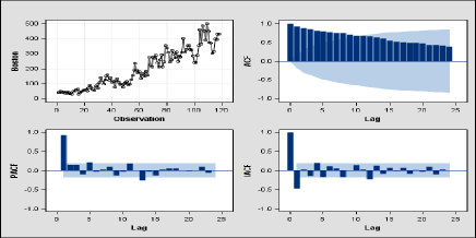
Figure 1: Boston armed robberies, time series (top left), autocorrelation function (top right), partial autocorrelation function (bottom left), inverse autocorrelation function (bottom right).

For preliminary fitting, subset ARIMA$(12,0,0)$ (Model 1) and ARIMA$(1,0,0)\times(1,0,0)_{12}$ (Model 2) models are applied. Here and in the sequel, ARIMA$(p,d,q)\times(P,D,Q)_{s}$ denotes a seasonal ARIMA model with period $s\in\mathbb{N}$ and orders $(p,d,q),(P,D,Q)\in\mathbb{Z}_{+}^{3}$, where capital letters denote the seasonal orders. We use the following approach to characterize the unstability of an ARIMA model. Let $a(B)$ and $A(B)$ be the autoregressive and seasonal autoregressive polynomial of the model, respectively, where $B$ denotes the backshift operator. We suppose that these polynomials are stable, i.e., the roots are all lie outside the complex unit circle. Define the coefficients $\alpha_{i}$, $i=1,\ldots,p+d+s(P+D)$, by $a(B)A(B)(1-B)^{d}(1-B^{s})^{D}=1-\sum_{i=1}^{p+d+s(P+D)}\alpha_{i}B^{i}$. Then, we characterize the unstability of the model by the sum $\Sigma:=\sum_{i=1}^{p+d+s(P+D)}\alpha_{i}$. Clearly, if an ARIMA model is unstable (nonstationary), i.e., $d>0$ or $D>0$, and hence its characteristic polynomial has unit root 1, then $\Sigma=1$. Since Model 1 is unstable and Model 2 is nearly unstable, see Table 1, Deutsch and Alt [15] suggested first order differencing and seasonal differencing getting an ARIMA$(0,1,1)\times(0,1,1)_{12}$ model (Model 3).

Model	Fitted model	$\Sigma$	Standard error
1	$(1-0.7865B-0.2135B^{12})X_{k}=\varepsilon_{k}+116.3733$	1	39.55
2	$(1-0.9783B)(1-0.2677B^{12})X_{k}=\varepsilon_{k}+49.2087$	0.9841	40.39
3	$(1-B)(1-B^{12})X_{k}=(1-0.5154B)(1-0.7345B^{12})\varepsilon_{k}+0.3181$	1	38.66
4	$(1-B)\ln X_{k}=(1-0.4345B)(1+0.1886B^{12})\varepsilon_{k}+0.0195$	1	0.1954
5	$X_{k}=0.6069\circ X_{k-1}+0.412\circ X_{k-12}+14.971+\widetilde{\varepsilon}_{k}$	1.0189	526.8
6	$X_{k}=0.682\circ X_{k-1}+0.3497\circ X_{k-12}+9.961+\widetilde{\varepsilon}_{k}$	1.0317	26.18

Table 1: Fitted models for Boston armed robberies data set with $\Sigma$ and standard error.

In contrast, Hay and McCleary [28] claimed that Deutsch and Alt had misspecified the stochastic component for this time series and they proposed only first order differencing getting an ARIMA$(0,1,1)\times(0,0,1)_{12}$ model (Model 4) after logarithmic transformation of the time series. Hay and McCleary reported that this alternative model has better statistical properties and there is no intervention into the time series (i.e., the parameters of the model do not vary in time), thus there is inconclusive evidence for the effect claimed by Deutsch and Alt. They argued for the need of logarithmic transformation to eliminate the “variance” nonstationarity of the time series. The following was reported by Hay and McCleary [28]: “We conducted several analyses to obtain supporting evidence for our hypothesis of variance nonstationarity. First, we divided the series into equal length segments and calculated the mean and standard deviation for each segment. Both statistics showed a nearly monotonic increase over time and were highly intercorrelated. Two tests of homogeneity of variance (Cochran’s C and the Bartlett and Box’s F) also indicated that the segment variances were not homogeneous.”

Based on the foregoing it is evident that the Boston armed robberies data set possesses the following properties: it is integer–valued, heteroscedastic, and unstable. Our aim here is to fit an appropriate INAR(p) model for this data set using the method of conditional least squares (CLS) and to compare our model with the previously mentioned ones. The CLS estimators $\widehat{\alpha}_{i}$, $i=1,\ldots,p$, and $\widehat{\mu_{\varepsilon}}$ of the parameters $\alpha_{i}$, $i=1,\ldots,p$, and $\mu_{\varepsilon}$ of an INAR$(p)$ model based on the observations $X_{1},\ldots,X_{n}$ are given by minimizing the residual sum of squares $\sum_{k=p+1}^{n}M_{k}^{2}$ in (3.10). This technique has been suggested by Klimko and Nelson [42] for general stochastic processes, and it has been applied for INAR$(p)$ models by Du and Li [19, Theorem 4.2] proving the asymptotic normality of these estimators in the stable case. The correlation analysis (Fig. 1) shows that there are significant dependences between $X_{k}$ and $X_{k-1}$, and, due to the seasonal effect, between $X_{k}$ and $X_{k-12}$. Thus, we fit a subset INAR$(12)$ model where the strictly positive coefficients are $\alpha_{1}$ and $\alpha_{12}$, and we estimate these (autoregressive) parameters and the mean $\mu_{\varepsilon}$. By solving the normal equations we have Model 5, see Table 1, where $\widetilde{\varepsilon}_{k}:=\varepsilon_{k}-\widehat{\mu_{\varepsilon}}$ is the centered innovation. Similarly to ARIMA models we characterize the unstability of an INAR$(p)$ model by the sum $\Sigma:=\sum_{i=1}^{p}\alpha_{i}$ (the classification of INAR(p) models is based on this sum, see the end of Section 2). Then the fitted Model 5 appears to be unstable since $\Sigma=1.0189$. For the goodness–of–fit of ARIMA and INAR models the standard error (the square root of the mean square error) is applied which is defined by $\operatorname{SE}:=((n-p-r)^{-1}\sum_{k=p+1}^{n}\widehat{M}_{k}^{2})^{1/2}$, where $\widehat{M}_{k}:=X_{k}-\sum_{i=1}^{p}\widehat{\alpha}_{i}X_{k-i}-\widehat{\mu_{\varepsilon}}$, $k=p+1,\ldots,n$, are the estimated residuals and $r$ denotes the number of estimated parameters. The standard error is relatively high for Model 5 ($\operatorname{SE}=526.8$) comparing with that of Deutsch and Alt’s model (Model 3) because the “error” terms $M_{k}$ fluctuate to much in (3.10) if the INAR model is unstable. (We note that the model of Hay and McCleary (Model 4) is uncomparable with the other ones using the standard error because of the logarithmic transformation has changed the scale.)

To stabilize the fluctuation of $M_{k}$ let us introduce the weighted martingale differences

$$M_{k}^{w}:=\frac{M_{k}}{\left(\sum_{\{j:\alpha_{j}>0\}}X_{k-j}+1\right)^{1/2}},\qquad k=p+1,\ldots,n.$$

Note that $\operatorname{E}(M_{k}^{w}\,|\,{\mathcal{F}}_{k-1})=0$ and, by (6.4),

$$\operatorname{E}\left((M_{k}^{w})^{2}\,\big{|}\,{\mathcal{F}}_{k-1}\right)=\frac{\sum_{\{j:\alpha_{j}>0\}}\alpha_{j}(1-\alpha_{j})X_{k-j}+\sigma_{\varepsilon}^{2}}{\sum_{\{j:\alpha_{j}>0\}}X_{k-j}+1},\qquad k=p+1,\ldots,n.$$

Since $\operatorname{E}\left((M_{k}^{w})^{2}\,\big{|}\,{\mathcal{F}}_{k-1}\right)\leq\sum_{\{j:\alpha_{j}>0\}}\alpha_{j}(1-\alpha_{j})+\sigma_{\varepsilon}^{2}$, the conditional variance of the “weighted error” terms $M_{k}^{w}$ would not fluctuate too much even if $(X_{k})_{k\in\mathbb{N}}$ is unbounded. Moreover, we have $\operatorname{E}\left((M_{k}^{w})^{2}\,\big{|}\,{\mathcal{F}}_{k-1}\right)\to\frac{1}{c}\sum_{j}\alpha_{j}(1-\alpha_{j})$ almost surely as $X_{k}\to\infty$ and $X_{k}/X_{k-1}\to 1$ almost surely, where  $c$  denotes the cardinality of the set  $\{j\in\{1,\ldots,p\}:\alpha_{j}>0\}$.  Hence, the weighted error terms $M_{k}^{w}$ are asymptotically homogeneous in the stable and the unstable cases as well. The weighted conditional least squares (WCLS) estimation is given by minimizing the weighted residual sum of squares $\sum_{k=p+1}^{n}(M_{k}^{w})^{2}$. This technique has been suggested by Wei and Winnicki [67] for branching processes with immigration to derive a unified estimation procedure for the offspring mean. By solving the normal equations we have Model 6 which appears to be unstable again, see Table 1. Defining the standard error for Model 6 as $\operatorname{SE}:=((n-p-r)^{-1}\sum_{k=p+1}^{n}(\widehat{M}_{k}^{w})^{2})^{1/2}$, this subset INAR(12) model possesses the smallest standard error among the fitted models except that of Hay and McCleary. The correlation analysis of estimated weighted residuals $\widehat{M}_{k}^{w}$, see Fig. 2, shows that they form a white noise time series.

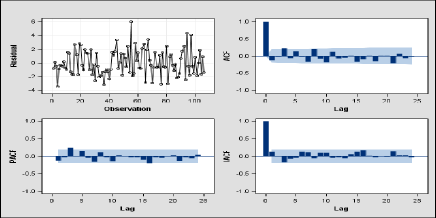
Figure 2: Residual analysis of Model 6, residual series (top left), autocorrelation function (top right), partial autocorrelation function (bottom left), inverse autocorrelation function (bottom right).

In summary, Model 6 is an adequate model for Boston armed robberies times series since its coefficients can be considered significant, it has minimum number of parameters and minimal residual variance (among the fitted models), and the residuals form a white noise. We note that the asymptotic theory of CLS and WCLS estimation of INAR$(p)$ models in the unstable case has not yet been developed now, this is a task for the future. Finally, we would like to call attention to other possible estimation methods which may also work in the unstable case. For example, Enciso–Mora et al. [20] proposed a reversible jump MCMC algorithm which even works well near the borders of the stationary region and has been successfully applied to a simulated nearly unstable INAR(3) data set having  $\Sigma=0.99$  as the sum of the (autoregressive) parameters.

5 Proof of Theorem 3.1

For the proof we will use Corollary 6.1, Theorem 6.1 and Lemma 6.2 which can be found in Appendix.

First we prove (3.7), i.e.,  ${\mathcal{M}}^{n}\stackrel{{\scriptstyle{\mathcal{L}}}}{{\longrightarrow}}{\mathcal{M}}$  as  $n\to\infty$.  We will apply Theorem 6.1 for  ${\mathcal{U}}={\mathcal{M}}$,  $U^{n}_{k}=n^{-1}M_{k}$,  $n,\,k\in\mathbb{N}$,  and for  $({\mathcal{F}}_{k}^{n})_{k\in\mathbb{Z}_{+}}=({\mathcal{F}}_{k})_{k\in\mathbb{Z}_{+}}$, $n\in\mathbb{N}$.  By Remark 3.4, the SDE (3.8) has a unique strong solution for all initial values  ${\mathcal{M}}^{x}_{0}=x$,  $x\in\mathbb{R}$.  Now we show that conditions (i) and (ii) of Theorem 6.1 hold. We have to check that for each  $T>0$,

(5.1) $$\sup_{t\in[0,T]}\bigg{|}\frac{1}{n^{2}}\sum_{k=1}^{{\lfloor nt\rfloor}}\operatorname{E}(M_{k}^{2}\,|\,{\mathcal{F}}_{k-1})-\frac{\sigma_{\alpha}^{2}}{\varphi^{\prime}(1)}\int_{0}^{t}({\mathcal{M}}^{n}_{s}+\mu_{\varepsilon}s)^{+}\,\mathrm{d}s\,\bigg{|}\stackrel{{\scriptstyle\operatorname{P}}}{{\longrightarrow}}0,$$

(5.2) $$\frac{1}{n^{2}}\sum_{k=1}^{{\lfloor nT\rfloor}}\operatorname{E}(M_{k}^{2}\mathbbm{1}_{\{|M_{k}|>n\theta\}}\,|\,{\mathcal{F}}_{k-1}\big{)}\stackrel{{\scriptstyle\operatorname{P}}}{{\longrightarrow}}0\qquad\text{for all \ $\theta>0$}$$

as  $n\to\infty$,  where  $\stackrel{{\scriptstyle\operatorname{P}}}{{\longrightarrow}}$  means convergence in probability.

By (3.6) and using also that  $\alpha_{1}+\cdots+\alpha_{p}=1$,  we get

$${\mathcal{M}}^{n}_{s}+\mu_{\varepsilon}s =n^{-1}\sum_{k=1}^{{\lfloor ns\rfloor}}\left(X_{k}-\sum_{i=1}^{p}\alpha_{i}X_{k-i}-\mu_{\varepsilon}\right)+\mu_{\varepsilon}s$$

$$=n^{-1}\left(\sum_{k={\lfloor ns\rfloor}-p+1}^{{\lfloor ns\rfloor}}X_{k}-\sum_{i=1}^{p-1}\alpha_{i}\sum_{k={\lfloor ns\rfloor}-p+1}^{{\lfloor ns\rfloor}-i}X_{k}\right)+\frac{ns-{\lfloor ns\rfloor}}{n}\mu_{\varepsilon}$$

$$=\frac{1}{n}\sum_{j=1}^{p}\sum_{i=j}^{p}\alpha_{i}X_{{\lfloor ns\rfloor}-j+1}+\frac{ns-{\lfloor ns\rfloor}}{n}\mu_{\varepsilon}.$$

Thus  $({\mathcal{M}}^{n}_{s}+\mu_{\varepsilon}s)^{+}={\mathcal{M}}^{n}_{s}+\mu_{\varepsilon}s$,  and using that

$$\int_{0}^{t}\frac{ns-{\lfloor ns\rfloor}}{n}\,\mathrm{d}s=\frac{t^{2}}{2}-\frac{1}{n}\left(\frac{1}{n}\sum_{k=1}^{{\lfloor nt\rfloor}-1}k+\left(t-\frac{{\lfloor nt\rfloor}}{n}\right){\lfloor nt\rfloor}\right)=\frac{{\lfloor nt\rfloor}+(nt-{\lfloor nt\rfloor})^{2}}{2n^{2}},$$

we get

$$\int_{0}^{t}({\mathcal{M}}^{n}_{s}+\mu_{\varepsilon}s)^{+}\,\mathrm{d}s =\frac{1}{n^{2}}\sum_{\ell=0}^{{\lfloor nt\rfloor}-1}\sum_{j=1}^{p}\sum_{i=j}^{p}\alpha_{i}X_{\ell-j+1}+\frac{nt-{\lfloor nt\rfloor}}{n^{2}}\sum_{j=1}^{p}\sum_{i=j}^{p}\alpha_{i}X_{{\lfloor nt\rfloor}-j+1}$$

$$\phantom{=\>}+\frac{{\lfloor nt\rfloor}+(nt-{\lfloor nt\rfloor})^{2}}{2n^{2}}\mu_{\varepsilon}.$$

Hence, using that  $\varphi^{\prime}(1)=\alpha_{1}+2\alpha_{2}+\cdots+p\alpha_{p}$,  we have

$$\int_{0}^{t}({\mathcal{M}}^{n}_{s}+\mu_{\varepsilon}s)^{+}\,\mathrm{d}s =\frac{\varphi^{\prime}(1)}{n^{2}}\sum_{\ell=0}^{{\lfloor nt\rfloor}-1}X_{\ell}-\frac{1}{n^{2}}\sum_{i=2}^{p}\alpha_{i}\sum_{j={\lfloor nt\rfloor}-i+1}^{{\lfloor nt\rfloor}-1}X_{j}$$

$$\phantom{=\>\;}+\frac{nt-{\lfloor nt\rfloor}}{n^{2}}\sum_{j=1}^{p}\sum_{i=j}^{p}\alpha_{i}X_{{\lfloor nt\rfloor}-j+1}+\frac{{\lfloor nt\rfloor}+(nt-{\lfloor nt\rfloor})^{2}}{2n^{2}}\mu_{\varepsilon}.$$

Using (6.4), we obtain

$$\frac{1}{n^{2}}\sum_{k=1}^{{\lfloor nt\rfloor}}\operatorname{E}(M_{k}^{2}\,|\,{\mathcal{F}}_{k-1}) =\frac{1}{n^{2}}\sum_{k=1}^{{\lfloor nt\rfloor}}\left(\sum_{i=1}^{p}\alpha_{i}(1-\alpha_{i})X_{k-i}+\sigma_{\varepsilon}^{2}\right)$$

$$=\frac{1}{n^{2}}\sum_{i=1}^{p}\left(\alpha_{i}(1-\alpha_{i})\sum_{j=1}^{{\lfloor nt\rfloor}-i+1}X_{j-1}\right)+\frac{{\lfloor nt\rfloor}}{n^{2}}\sigma_{\varepsilon}^{2}$$

$$=\frac{\sigma_{\alpha}^{2}}{n^{2}}\sum_{k=1}^{{\lfloor nt\rfloor}}X_{k-1}-\frac{1}{n^{2}}\sum_{i=2}^{p}\left(\alpha_{i}(1-\alpha_{i})\sum_{j={\lfloor nt\rfloor}-i+1}^{{\lfloor nt\rfloor}-1}X_{j}\right)+\frac{{\lfloor nt\rfloor}}{n^{2}}\sigma_{\varepsilon}^{2}.$$

Hence, for all  $n\in\mathbb{N}$,  the randomness of the difference in (5.1) is via a linear combination of the random variables  $X_{{\lfloor nt\rfloor}-j}$, $j=1,\ldots,p$.  Then, in order to show (5.1), it suffices to prove

(5.3) $$\sup_{t\in[0,T]}\frac{1}{n^{2}}X_{{\lfloor nt\rfloor}}\stackrel{{\scriptstyle\operatorname{P}}}{{\longrightarrow}}0\qquad\text{as \ $n\to\infty$.}$$

By (3.11) and (6.8),

$$X_{{\lfloor nt\rfloor}}\leqslant\sum_{j=1}^{{\lfloor nt\rfloor}}|M_{j}+\mu_{\varepsilon}|\cdot\|{\boldsymbol{A}}^{{\lfloor nt\rfloor}-j}\|\leqslant C_{\boldsymbol{A}}\biggl{(}{\lfloor nt\rfloor}\cdot\mu_{\varepsilon}+\sum_{j=1}^{{\lfloor nt\rfloor}}|M_{j}|\biggr{)}.$$

Consequently, in order to prove (5.3), it suffices to show

$$\frac{1}{n^{2}}\sum_{j=1}^{{\lfloor nT\rfloor}}|M_{j}|\stackrel{{\scriptstyle\operatorname{P}}}{{\longrightarrow}}0\qquad\text{as \ $n\to\infty$.}$$

In fact, one can show that  $n^{-2}\sum_{j=1}^{{\lfloor nT\rfloor}}\operatorname{E}(|M_{j}|)\to 0$.  Indeed, Corollary 6.1 yields that

$$n^{-2}\sum_{j=1}^{{\lfloor nT\rfloor}}\operatorname{E}(|M_{j}|)\leqslant\frac{K}{n^{2}}\sum_{j=1}^{{\lfloor nT\rfloor}}\sqrt{j}\leqslant\frac{K}{n^{2}}{\lfloor nT\rfloor}\sqrt{{\lfloor nT\rfloor}}\to 0\quad\text{as \ $n\to\infty$,}$$

with some constant  $K\in\mathbb{R}_{+}$.  Thus we obtain (5.1).

To prove (5.2), consider the decomposition  $M_{k}=N_{k}+(\varepsilon_{k}-\mu_{\varepsilon})$,  where, by (6.7),

$$N_{k}:=\sum_{\ell=1}^{X_{k-1}}(\xi_{k,1,\ell}-\operatorname{E}(\xi_{k,1,\ell}))+\cdots+\sum_{\ell=1}^{X_{k-p}}(\xi_{k,p,\ell}-\operatorname{E}(\xi_{k,p,\ell})).$$

Clearly,

$$M_{k}^{2}\leqslant 2\big{(}N_{k}^{2}+(\varepsilon_{k}-\mu_{\varepsilon})^{2}\big{)}\qquad\text{and}\qquad\mathbbm{1}_{\{|M_{k}|>n\theta\}}\leqslant\mathbbm{1}_{\{|N_{k}|>n\theta/2\}}+\mathbbm{1}_{\{|\varepsilon_{k}-\mu_{\varepsilon}|>n\theta/2\}},$$

and hence (5.2) will be proved once we show

(5.4) $$\frac{1}{n^{2}}\sum_{k=1}^{{\lfloor nT\rfloor}}\operatorname{E}(N_{k}^{2}\mathbbm{1}_{\{|N_{k}|>n\theta\}}\,|\,{\mathcal{F}}_{k-1})\stackrel{{\scriptstyle\operatorname{P}}}{{\longrightarrow}}0\qquad\text{for all \ $\theta>0$,}$$

(5.5) $$\frac{1}{n^{2}}\sum_{k=1}^{{\lfloor nT\rfloor}}\operatorname{E}(N_{k}^{2}\mathbbm{1}_{\{|\varepsilon_{k}-\mu_{\varepsilon}|>n\theta\}}\,|\,{\mathcal{F}}_{k-1})\stackrel{{\scriptstyle\operatorname{P}}}{{\longrightarrow}}0\qquad\text{for all \ $\theta>0$,}$$

(5.6) $$\frac{1}{n^{2}}\sum_{k=1}^{{\lfloor nT\rfloor}}\operatorname{E}((\varepsilon_{k}-\mu_{\varepsilon}))^{2}\,|\,{\mathcal{F}}_{k-1})\stackrel{{\scriptstyle\operatorname{P}}}{{\longrightarrow}}0.$$

First we prove (5.4). Using that the random variables  $\{\xi_{k,i,j}:j\in\mathbb{N},\,i\in\{1,\ldots,p\}\}$  are independent of the  $\sigma$-algebra  ${\mathcal{F}}_{k-1}$  for all  $k\in\mathbb{N}$,  we get

$$\operatorname{E}(N_{k}^{2}\mathbbm{1}_{\{|N_{k}|>n\theta\}}\,|\,{\mathcal{F}}_{k-1})=F_{k}(X_{k-1},\ldots,X_{k-p}),$$

where  $F_{k}:\mathbb{Z}_{+}^{p}\to\mathbb{R}$  is given by

$$F_{k}(z_{1},\dots,z_{p}):=\operatorname{E}((S_{k}(z_{1},\dots,z_{p})^{2}\mathbbm{1}_{\{|S_{k}(z_{1},\dots,z_{p})|>n\theta\}})),\qquad z_{1},\ldots,z_{p}\in\mathbb{Z}_{+},$$

with  $S_{k}(z_{1},\dots,z_{p}):=\sum_{i=1}^{p}\sum_{\ell=1}^{z_{i}}(\xi_{k,i,\ell}-\operatorname{E}(\xi_{k,i,\ell}))$.  Consider the decomposition

$$F_{k}(z_{1},\dots,z_{p})=A_{k}(z_{1},\dots,z_{p})+B_{k}(z_{1},\dots,z_{p}),$$

where

$$A_{k}(z_{1},\dots,z_{p}) :=\sum_{i=1}^{p}\sum_{\ell=1}^{z_{i}}\operatorname{E}((\xi_{k,i,\ell}-\operatorname{E}(\xi_{k,i,\ell}))^{2}\mathbbm{1}_{\{|S_{k}(z_{1},\dots,z_{p})|>n\theta\}}),$$

$$B_{k}(z_{1},\dots,z_{p}) :=\sum\nolimits^{\prime}\operatorname{E}((\xi_{k,i,\ell}-\operatorname{E}(\xi_{k,i,\ell}))(\xi_{k,j,\ell^{\prime}}-\operatorname{E}(\xi_{k,j,\ell^{\prime}}))\mathbbm{1}_{\{|S_{k}(z_{1},\dots,z_{p})|>n\theta\}}),$$

where the sum  $\sum^{\prime}$  is taken for  $i,j=1,\dots,p$,  $\ell=1,\dots,z_{i}$,  $\ell^{\prime}=1,\dots,z_{j}$  with  $(i,\ell)\not=(j,\ell^{\prime})$.  Consider the decompositions

$$S_{k}(z_{1},\dots,z_{p})=(\xi_{k,i,\ell}-\operatorname{E}(\xi_{k,i,\ell}))+\widetilde{S}^{i}_{k,\ell}(z_{1},\dots,z_{p}),\qquad i=1,\ldots,p,\;\;\ell=1,\ldots,z_{i},$$

where

$$\widetilde{S}^{i}_{k,\ell}(z_{1},\dots,z_{p}):=\sum\nolimits^{\prime\prime}\big{(}\xi_{k,j,\ell^{\prime}}-\operatorname{E}(\xi_{k,j,\ell^{\prime}})\big{)},$$

where the sum  $\sum^{\prime\prime}$  is taken for  $j=1,\dots,p$  and  $\ell^{\prime}=1,\dots,z_{j}$  with  $(j,\ell^{\prime})\not=(i,\ell)$.

Using that

$$\mathbbm{1}_{\{|S_{k}(z_{1},\dots,z_{p})|>n\theta\}}\leqslant\mathbbm{1}_{\{|\xi_{k,i,\ell}-\operatorname{E}(\xi_{k,i,\ell})|>n\theta/2\}}+\mathbbm{1}_{\{|\widetilde{S}^{i}_{k,\ell}(z_{1},\dots,z_{p})|>n\theta/2\}},$$

we have

$$A_{k}(z_{1},\dots,z_{p})\leqslant A_{k}^{(1)}(z_{1},\dots,z_{p})+A_{k}^{(2)}(z_{1},\dots,z_{p}),$$

where

$$A_{k}^{(1)}(z_{1},\dots,z_{p}) :=\sum_{i=1}^{p}\sum_{\ell=1}^{z_{i}}\operatorname{E}((\xi_{k,i,\ell}-\operatorname{E}(\xi_{k,i,\ell}))^{2}\mathbbm{1}_{\{|\xi_{k,i,\ell}-\operatorname{E}(\xi_{k,i,\ell})|>n\theta/2\}}),$$

$$A_{k}^{(2)}(z_{1},\dots,z_{p}) :=\sum_{i=1}^{p}\sum_{\ell=1}^{z_{i}}\operatorname{E}((\xi_{k,i,\ell}-\operatorname{E}(\xi_{k,i,\ell}))^{2}\mathbbm{1}_{\{|\widetilde{S}^{i}_{k,\ell}(z_{1},\dots,z_{p})|>n\theta/2\}}).$$

In order to prove (5.4), it is enough to show that

$$\frac{1}{n^{2}}\sum_{k=1}^{{\lfloor nT\rfloor}}A_{k}^{(1)}(X_{k-1},\ldots,X_{k-p})\stackrel{{\scriptstyle\operatorname{P}}}{{\longrightarrow}}0,\qquad\qquad\frac{1}{n^{2}}\sum_{k=1}^{{\lfloor nT\rfloor}}A_{k}^{(2)}(X_{k-1},\ldots,X_{k-p})\stackrel{{\scriptstyle\operatorname{P}}}{{\longrightarrow}}0,$$

(5.7) $$\frac{1}{n^{2}}\sum_{k=1}^{{\lfloor nT\rfloor}}B_{k}(X_{k-1},\dots,X_{k-p})\stackrel{{\scriptstyle\operatorname{P}}}{{\longrightarrow}}0$$

as  $n\to\infty$.  We have

$$A_{k}^{(1)}(z_{1},\dots,z_{p})=\sum_{i=1}^{p}z_{i}\operatorname{E}((\xi_{1,i,1}-\operatorname{E}(\xi_{1,i,1}))^{2}\mathbbm{1}_{\{|\xi_{1,i,1}-\operatorname{E}(\xi_{1,i,1})|>n\theta/2\}}),\qquad k\in\mathbb{N},$$

where

$$\operatorname{E}((\xi_{1,i,1}-\operatorname{E}(\xi_{1,i,1}))^{2}\mathbbm{1}_{\{|\xi_{1,i,1}-\operatorname{E}(\xi_{1,i,1})|>n\theta/2\}})\to 0,$$

as  $n\to\infty$  for all  $i\in\{1,\dots,p\}$  by the dominated convergence theorem. Thus, by Corollary 6.1, we get with some constant  $K\in\mathbb{R}_{+}$,

$$\frac{1}{n^{2}}\sum_{k=1}^{{\lfloor nT\rfloor}} \operatorname{E}(A_{k}^{(1)}(X_{k-1},\dots,X_{k-p}))$$

$$=\frac{1}{n^{2}}\sum_{k=1}^{{\lfloor nT\rfloor}}\sum_{i=1}^{p}\operatorname{E}(X_{k-i})\operatorname{E}((\xi_{1,i,1}-\operatorname{E}(\xi_{1,i,1}))^{2}\mathbbm{1}_{\{|\xi_{1,i,1}-\operatorname{E}(\xi_{1,i,1})|>n\theta/2\}})$$

$$\leqslant\sum_{i=1}^{p}\left[\operatorname{E}((\xi_{1,i,1}-\operatorname{E}(\xi_{1,i,1}))^{2}\mathbbm{1}_{\{|\xi_{1,i,1}-\operatorname{E}(\xi_{1,i,1})|>n\theta/2\}})\frac{K}{n^{2}}\sum_{k=i+1}^{{\lfloor nT\rfloor}}(k-i)\right]$$

$$\leqslant K\frac{{\lfloor nT\rfloor}({\lfloor nT\rfloor}+1)}{2n^{2}}\sum_{i=1}^{p}\operatorname{E}((\xi_{1,i,1}-\operatorname{E}(\xi_{1,i,1}))^{2}\mathbbm{1}_{\{|\xi_{1,i,1}-\operatorname{E}(\xi_{1,i,1})|>n\theta/2\}})\to 0,$$

which yields  $n^{-2}\sum_{k=1}^{{\lfloor nT\rfloor}}A_{k}^{(1)}(X_{k-1},\dots,X_{k-p})\stackrel{{\scriptstyle\operatorname{P}}}{{\longrightarrow}}0$.

Independence of  $\xi_{k,i,\ell}-\operatorname{E}(\xi_{k,i,\ell})$  and  $\widetilde{S}^{i}_{k,\ell}(z_{1},\dots,z_{p})$  implies

$$A_{k}^{(2)}(z_{1},\dots,z_{p})=\sum_{i=1}^{p}\sum_{\ell=1}^{z_{i}}\operatorname{E}((\xi_{k,i,\ell}-\operatorname{E}(\xi_{k,i,\ell}))^{2})\operatorname{P}(|\widetilde{S}^{i}_{k,\ell}(z_{1},\dots,z_{d})|>n\theta/2\big{)}.$$

Here  $\operatorname{E}((\xi_{k,i,\ell}-\operatorname{E}(\xi_{k,i,\ell}))^{2})=\alpha_{i}(1-\alpha_{i})$, $i=1,\ldots,p$,  and, by Markov’s inequality,

$$\operatorname{P}(|\widetilde{S}^{i}_{k,\ell}(z_{1},\dots,z_{p})|>n\theta/2)\leqslant\frac{4}{n^{2}\theta^{2}}\operatorname{E}(\widetilde{S}^{i}_{k,\ell}(z_{1},\dots,z_{p})^{2})\\ =\frac{4}{n^{2}\theta^{2}}\operatorname{Var}(\widetilde{S}^{i}_{k,\ell}(z_{1},\dots,z_{p}))=\frac{4}{n^{2}\theta^{2}}\sum\nolimits^{\prime\prime}\alpha_{j}(1-\alpha_{j})\leqslant\frac{4}{n^{2}\theta^{2}}\sum_{j=1}^{p}z_{j}\alpha_{j}(1-\alpha_{j}).$$

Thus we get

$$A_{k}^{(2)}(z_{1},\dots,z_{p})\leqslant\frac{4}{n^{2}\theta^{2}}\sum_{i=1}^{p}\sum_{j=1}^{p}z_{i}z_{j}\alpha_{i}(1-\alpha_{i})\alpha_{j}(1-\alpha_{j}).$$

Hence, by Cauchy-Schwarz’s inequality and Corollary 6.1, we get with some constant  $K\in\mathbb{R}_{+}$,

$$\frac{1}{n^{2}}\sum_{k=1}^{{\lfloor nT\rfloor}}\operatorname{E}(A_{k}^{(2)}(X_{k-1},\ldots,X_{k-p})) \leqslant\frac{4}{n^{4}\theta}\sum_{k=1}^{{\lfloor nT\rfloor}}\sum_{i=1}^{p}\sum_{j=1}^{p}\operatorname{E}(X_{k-i}X_{k-j})\alpha_{i}(1-\alpha_{i})\alpha_{j}(1-\alpha_{j})$$

$$\leqslant\frac{4K}{n^{4}\theta}\sum_{k=1}^{{\lfloor nT\rfloor}}k^{2}\left(\sum_{i=1}^{p}\alpha_{i}(1-\alpha_{i})\right)^{2}\to 0,$$

which implies  $n^{-2}\sum_{k=1}^{{\lfloor nT\rfloor}}A_{k}^{(2)}(X_{k-1},\ldots,X_{k-p})\stackrel{{\scriptstyle\operatorname{P}}}{{\longrightarrow}}0$.

By Cauchy-Schwarz’s inequality,

$$|B_{k}(z_{1},\dots,z_{p})|\leqslant\sqrt{B_{k}^{(1)}(z_{1},\dots,z_{p})\,\operatorname{E}(\mathbbm{1}_{\{|S_{k}(z_{1},\dots,z_{p})|>n\theta\}})},$$

where

$$B_{k}^{(1)}(z_{1},\dots,z_{p}):=\operatorname{E}\bigg{(}\Big{(}\sum\nolimits^{\prime}(\xi_{k,i,\ell}-\operatorname{E}(\xi_{k,i,\ell}))(\xi_{k,j,\ell^{\prime}}-\operatorname{E}(\xi_{k,j,\ell^{\prime}}))\Big{)}^{2}\bigg{)},\qquad z_{1},\ldots,z_{p}\in\mathbb{Z}_{+}.$$

Using the independence of  $\xi_{k,i,\ell}-\operatorname{E}(\xi_{k,i,\ell})$  and  $\xi_{k,j,\ell^{\prime}}-\operatorname{E}(\xi_{k,j,\ell^{\prime}})$  for  $(i,\ell)\neq(j,\ell^{\prime})$,  we get

$$B_{k}^{(1)}(z_{1},\dots,z_{p}) =\sum\nolimits^{\prime}\alpha_{i}(1-\alpha_{i})\alpha_{j}(1-\alpha_{j})$$

$$=\sum_{i=1}^{p}z_{i}(z_{i}-1)\alpha_{i}^{2}(1-\alpha_{i})^{2}+\sum_{i\neq j}z_{i}z_{j}\alpha_{i}(1-\alpha_{i})\alpha_{j}(1-\alpha_{j})$$

$$\leqslant K_{1}(z_{1}+\cdots+z_{p})^{2},$$

with some constant  $K_{1}\in\mathbb{R}_{+}$.  Further, by Markov’s inequality,

$$\operatorname{E}(\mathbbm{1}_{\{|S_{k}(z_{1},\dots,z_{p})|>n\theta\}})\leqslant\frac{1}{n^{2}\theta^{2}}\sum_{j=1}^{p}z_{j}\alpha_{j}(1-\alpha_{j})\leqslant\frac{K_{2}}{n^{2}\theta^{2}}(z_{1}+\dots+z_{p}),$$

with some constant  $K_{2}\in\mathbb{R}_{+}$.  Hence

$$|B_{k}(z_{1},\dots,z_{p})|\leqslant\frac{K}{n}(z_{1}+\dots+z_{p})^{3/2},\qquad z_{1},\ldots,z_{p}\in\mathbb{Z}_{+},$$

with some constant  $K\in\mathbb{R}_{+}$.  Using that

$$(z_{1}+\dots+z_{p})^{3/2}\leqslant c_{p}(z_{1}^{3/2}+\dots+z_{p}^{3/2}),\qquad z_{1},\ldots,z_{p}\in\mathbb{Z}_{+},$$

with some constant  $c_{p}\in\mathbb{R}_{+}$,  we get, in order to show (5.7), it suffices to prove  $n^{-3}\sum_{k=1}^{{\lfloor nT\rfloor}}\big{(}X_{k-1}^{3/2}+\cdots+X_{k-p}^{3/2}\big{)}\stackrel{{\scriptstyle\operatorname{P}}}{{\longrightarrow}}0$.  In fact,  $n^{-3}\sum_{k=1}^{{\lfloor nT\rfloor}}\big{(}\operatorname{E}(X_{k-1}^{3/2})+\cdots+\operatorname{E}(X_{k-p}^{3/2})\big{)}\to 0$  since Corollary 6.1 implies  $\operatorname{E}(X_{\ell}^{3/2})\leqslant\big{(}\operatorname{E}(X_{\ell}^{2})\big{)}^{3/4}=O(\ell^{3/2})$.  Thus we finished the proof of (5.4).

Now we turn to prove (5.5). Using that for all  $k\in\mathbb{N}$  the random variables  $\{\xi_{k,i,j},\,\varepsilon_{k}:j\in\mathbb{N},\,i\in\{1,\ldots,p\}\}$  are independent of the  $\sigma$-algebra  ${\mathcal{F}}_{k-1}$,  we get  $\operatorname{E}(N_{k}^{2}\mathbbm{1}_{\{|\varepsilon_{k}-\mu_{\varepsilon}|>n\theta\}}\,|\,{\mathcal{F}}_{k-1})=G_{k}(X_{k-1},\ldots,X_{k-p})$,  where  $G_{k}:\mathbb{Z}_{+}^{p}\to\mathbb{R}$  is given by

$$G_{k}(z_{1},\dots,z_{p}):=\operatorname{E}(S_{k}(z_{1},\dots,z_{p})^{2}\mathbbm{1}_{\{|\varepsilon_{k}-\mu_{\varepsilon}|>n\theta\}}\big{)},\qquad z_{1},\ldots,z_{p}\in\mathbb{Z}_{+}.$$

Using again the independence of  $\big{\{}\xi_{k,i,j},\,\varepsilon_{k}:j\in\mathbb{N},\,i\in\{1,\dots,p\}\big{\}}$,

$$G_{k}(z_{1},\dots,z_{p})=\operatorname{P}(|\varepsilon_{k}-\mu_{\varepsilon}|>n\theta)\sum_{i=1}^{p}\sum_{\ell=1}^{z_{i}}\operatorname{E}((\xi_{k,i,\ell}-\operatorname{E}(\xi_{k,i,\ell}))^{2}),$$

where by Markov’s inequality,  $\operatorname{P}(|\varepsilon_{k}-\mu_{\varepsilon}|>n\theta\big{)}\leqslant n^{-2}\theta^{-2}\operatorname{E}((\varepsilon_{k}-\mu_{\varepsilon})^{2})=n^{-2}\theta^{-2}\sigma_{\varepsilon}^{2}$ ,  and  $\operatorname{E}((\xi_{k,i,\ell}-\operatorname{E}(\xi_{k,i,\ell}))^{2})=\alpha_{i}(1-\alpha_{i})$.  Hence, in order to show (5.5), it suffices to prove  $n^{-4}\sum_{k=1}^{{\lfloor nT\rfloor}}X_{k}\stackrel{{\scriptstyle\operatorname{P}}}{{\longrightarrow}}0$.  In fact, by Corollary 6.1,  $n^{-4}\sum_{k=1}^{{\lfloor nT\rfloor}}\operatorname{E}(X_{k})\to 0$.

Now we turn to prove (5.6). By independence of  $\varepsilon_{k}$  and  ${\mathcal{F}}_{k-1}$,

$$\frac{1}{n^{2}}\sum_{k=1}^{{\lfloor nT\rfloor}}\operatorname{E}((\varepsilon_{k}-\mu_{\varepsilon})^{2}\,|\,{\mathcal{F}}_{k-1})=\frac{1}{n^{2}}\sum_{k=1}^{{\lfloor nT\rfloor}}\operatorname{E}((\varepsilon_{k}-\mu_{\varepsilon})^{2})=\frac{{\lfloor nT\rfloor}}{n^{2}}\sigma_{\varepsilon}^{2}\to 0,$$

thus we obtain (5.6). Hence we get (5.2), and we conclude, by Theorem 6.1, convergence  ${\mathcal{M}}_{n}\stackrel{{\scriptstyle{\mathcal{L}}}}{{\longrightarrow}}{\mathcal{M}}$.

Now we start to prove (3.1). By (3.11),  ${\mathcal{X}}^{n}=\Psi_{n}({\mathcal{M}}^{n})$,  where the mapping  $\Psi_{n}:\mathsf{D}(\mathbb{R}_{+},\mathbb{R})\to\mathsf{D}(\mathbb{R}_{+},\mathbb{R})$  is given by

$$\Psi_{n}(f)(t):=\sum_{j=1}^{\lfloor nt\rfloor}\left(f\left(\frac{j}{n}\right)-f\left(\frac{j-1}{n}\right)+\frac{\mu_{\varepsilon}}{n}\right){\boldsymbol{e}}_{1}^{\top}{\boldsymbol{A}}^{{\lfloor nt\rfloor}-j}{\boldsymbol{e}}_{1}$$

for  $f\in\mathsf{D}(\mathbb{R}_{+},\mathbb{R})$,  $t\in\mathbb{R}_{+}$,  $n\in\mathbb{N}$.  Further,  ${\mathcal{X}}=\Psi({\mathcal{M}})$,  where, by (3.9), the mapping  $\Psi:\mathsf{D}(\mathbb{R}_{+},\mathbb{R})\to\mathsf{D}(\mathbb{R}_{+},\mathbb{R})$  is given by

$$\Psi(f)(t):=\frac{1}{\varphi^{\prime}(1)}\big{(}f(t)+\mu_{\varepsilon}t\big{)},\qquad f\in\mathsf{D}(\mathbb{R}_{+},\mathbb{R}),\quad t\in\mathbb{R}_{+}.$$

We check that the mappings  $\Psi_{n}$, $n\in\mathbb{N}$,  and  $\Psi$  are measurable. Continuity of  $\Psi$  follows from the characterization of convergence in  $\mathsf{D}(\mathbb{R}_{+},\mathbb{R})$,  see, e.g., Ethier and Kurtz [21, Proposition 3.5.3], thus we obtain measurability of  $\Psi$.  Indeed, if  $f_{n}\in\mathsf{D}(\mathbb{R}_{+},\mathbb{R})$, $n\in\mathbb{N}$,  $f\in\mathsf{D}(\mathbb{R}_{+},\mathbb{R})$  and the sequence  $(f_{n})_{n\in\mathbb{N}}$  converges in  $\mathsf{D}(\mathbb{R}_{+},\mathbb{R})$  to  $f$,  then for all  $T>0$  there exist continuous, increasing mappings  $\lambda_{n}$, $n\in\mathbb{N}$,  from  $[0,\infty)$  onto  $[0,\infty)$  such that

$$\lim_{n\to\infty}\sup_{t\in[0,T]}|\lambda_{n}(t)-t|=0\qquad\text{and}\qquad\lim_{n\to\infty}\sup_{t\in[0,T]}|f_{n}(\lambda_{n}(t))-f(t)|=0.$$

Since for all  $t\in\mathbb{R}_{+}$

$$|\Psi(f_{n})(\lambda_{n}(t))-\Psi(f)(t)| =\left|\frac{1}{\varphi^{\prime}(1)}(f_{n}(\lambda_{n}(t))+\mu_{\varepsilon}\lambda_{n}(t))-\frac{1}{\varphi^{\prime}(1)}(f(t)+\mu_{\varepsilon}t)\right|$$

$$\leqslant\frac{1}{\varphi^{\prime}(1)}|f_{n}(\lambda_{n}(t))-f(t)|+\frac{\mu_{\varepsilon}}{\varphi^{\prime}(1)}|\lambda_{n}(t)-t|,$$

we have for all  $T>0$,

$$\lim_{n\to\infty}\sup_{t\in[0,T]}|\Psi(f_{n})(\lambda_{n}(t))-\Psi(f)(t)|=0.$$

In order to prove measurability of  $\Psi_{n}$,  first we localize it. For each  $N\in\mathbb{N}$,  consider the stopped mapping  $\Psi^{N}_{n}:\mathsf{D}(\mathbb{R}_{+},\mathbb{R})\to\mathsf{D}(\mathbb{R}_{+},\mathbb{R})$  given by  $\Psi^{N}_{n}(f)(t):=\Psi_{n}(f)(t\land N)$  for  $f\in\mathsf{D}(\mathbb{R}_{+},\mathbb{R})$,  $t\in\mathbb{R}_{+}$,  $n,N\in\mathbb{N}$. Obviously,  $\Psi^{N}_{n}(f)\to\Psi_{n}(f)$  in  $\mathsf{D}(\mathbb{R}_{+},\mathbb{R})$  as  $N\to\infty$  for all  $f\in\mathsf{D}(\mathbb{R}_{+},\mathbb{R})$,  since for all  $T>0$  and  $N\geqslant T$  we have  $\Psi^{N}_{n}(f)(t):=\Psi_{n}(f)(t)$, $t\in[0,T]$,  and hence  $\sup_{t\in[0,T]}|\Psi^{N}_{n}(f)(t)-\Psi_{n}(f)(t)|\to 0$  as  $N\to\infty$.  Consequently, it suffices to show measurability of  $\Psi^{N}_{n}$  for all  $n,N\in\mathbb{N}$.  We can write  $\Psi^{N}_{n}=\Psi^{N,2}_{n}\circ\Psi^{N,1}_{n}$,  where the mappings  $\Psi^{N,1}_{n}:\mathsf{D}(\mathbb{R}_{+},\mathbb{R})\to\mathbb{R}^{nN+1}$  and  $\Psi^{N,2}_{n}:\mathbb{R}^{nN+1}\to\mathsf{D}(\mathbb{R}_{+},\mathbb{R})$  are defined by

$$\Psi_{n}^{N,1}(f) :=\left(f(0),f\left(\frac{1}{n}\right),f\left(\frac{2}{n}\right),\dots,f(N)\right),$$

$$\Psi_{n}^{N,2}(x_{0},x_{1},\dots,x_{nN})(t) :=\sum_{j=1}^{\lfloor n(t\land N)\rfloor}\left(x_{j}-x_{j-1}+\frac{\mu_{\varepsilon}}{n}\right){\boldsymbol{e}}_{1}^{\top}{\boldsymbol{A}}^{{\lfloor nt\rfloor}-j}{\boldsymbol{e}}_{1}$$

for  $f\in\mathsf{D}(\mathbb{R}_{+},\mathbb{R})$,  $t\in\mathbb{R}_{+}$,  $x=(x_{0},x_{1},\dots,x_{nN})\in\mathbb{R}^{nN+1}$,  $n,N\in\mathbb{N}$.  Measurability of  $\Psi^{N,1}_{n}$  follows from Ethier and Kurtz [21, Proposition 3.7.1]. Next we show continuity of  $\Psi^{N,2}_{n}$  by checking  $\sup_{t\in[0,T]}|\Psi^{N,2}_{n}(x^{k})(t)-\Psi^{N,2}_{n}(x)(t)|\to 0$  as  $k\to\infty$  for all  $T>0$  whenever  $x^{k}\to x$  in  $\mathbb{R}^{nN+1}$.  This convergence follows from the estimates

$$\sup_{t\in[0,T]}|\Psi^{N,2}_{n}(x^{k})(t)-\Psi^{N,2}_{n}(x)(t)|\leqslant\sum_{j=1}^{\lfloor n(T\land N)\rfloor}\bigl{(}|x^{k}_{j}-x_{j}|+|x^{k}_{j-1}-x_{j-1}|\bigr{)}\left|{\boldsymbol{e}}_{1}^{\top}{\boldsymbol{A}}^{{\lfloor nt\rfloor}-j}{\boldsymbol{e}}_{1}\right|,$$

since  $\left|{\boldsymbol{e}}_{1}^{\top}{\boldsymbol{A}}^{{\lfloor nt\rfloor}-j}{\boldsymbol{e}}_{1}\right|\leqslant\|{\boldsymbol{A}}^{{\lfloor nt\rfloor}-j}\|\leqslant C_{A}$. We obtain measurability of both  $\Psi^{N,1}_{n}$  and  $\Psi^{N,2}_{n}$,  hence we conclude measurability of  $\Psi^{N}_{n}$.  The aim of the following discussion is to show that there exists  $C\subset C_{\Psi,(\Psi_{n})_{n\in\mathbb{N}}}$  with  $C\in{\mathcal{D}}_{\infty}$  and  $P({\mathcal{M}}\in C)=1$,  where  $C_{\Psi,(\Psi_{n})_{n\in\mathbb{N}}}$  is defined in Appendix. We check that  $C:=\{f\in\mathsf{C}(\mathbb{R}_{+},\mathbb{R}):f(0)=0\}$  satisfies the above mentioned conditions. First note that  $C=\mathsf{C}(\mathbb{R}_{+},\mathbb{R})\cap\pi_{0}^{-1}(0)$,  where  $\pi_{0}:\mathsf{D}(\mathbb{R}_{+},\mathbb{R})\to\mathbb{R}$,  $\pi_{0}(f):=f(0),$ $f\in\mathsf{D}(\mathbb{R}_{+},\mathbb{R})$. Using that  $\mathsf{C}(\mathbb{R}_{+},\mathbb{R})$  is a measurable subset of  $\mathsf{D}(\mathbb{R}_{+},\mathbb{R})$  (see, e.g., Ethier and Kurtz [21, Problem 3.11.25]) and that  $\pi_{0}$  is measurable (see, e.g., Ethier and Kurtz [21, Proposition 3.7.1]), we have  $C\in{\mathcal{D}}_{\infty}$.  Fix a function  $f\in\mathsf{C}(\mathbb{R}_{+},\mathbb{R})$  and a sequence  $(f_{n})_{n\in\mathbb{N}}$  in  $\mathsf{D}(\mathbb{R}_{+},\mathbb{R})$  with  $f_{n}\stackrel{{\scriptstyle{\scriptstyle\mathrm{lu}}}}{{\longrightarrow}}f$,  where  $\stackrel{{\scriptstyle{\scriptstyle\mathrm{lu}}}}{{\longrightarrow}}$  is defined in Appendix. By the definition of  $\Psi$,  we get  $\Psi(f)\in\mathsf{C}(\mathbb{R}_{+},\mathbb{R})$.  Further, we can write

$$\Psi_{n}(f_{n})(t) =\sum_{j=1}^{\lfloor nt\rfloor}\left(f_{n}\left(\frac{j}{n}\right)-f_{n}\left(\frac{j-1}{n}\right)+\frac{\mu_{\varepsilon}}{n}\right){\boldsymbol{e}}_{1}^{\top}{\boldsymbol{\Pi}}_{\boldsymbol{A}}{\boldsymbol{e}}_{1}$$

$$\phantom{=\>}+\sum_{j=1}^{\lfloor nt\rfloor}\left(f_{n}\left(\frac{j}{n}\right)-f_{n}\left(\frac{j-1}{n}\right)+\frac{\mu_{\varepsilon}}{n}\right){\boldsymbol{e}}_{1}^{\top}({\boldsymbol{A}}^{{\lfloor nt\rfloor}-j}-{\boldsymbol{\Pi}}_{\boldsymbol{A}}){\boldsymbol{e}}_{1},\qquad t\in\mathbb{R}_{+}.$$

Using (2.10) and the assumption  $\varrho(A)=\alpha_{1}+\cdots+\alpha_{p}=1$, we get  ${\boldsymbol{e}}_{1}^{\top}{\boldsymbol{\Pi}}_{\boldsymbol{A}}{\boldsymbol{e}}_{1}=\frac{1}{\varphi^{\prime}(1)}$  and

$$\sum_{j=1}^{\lfloor nt\rfloor}\left(f_{n}\left(\frac{j}{n}\right)-f_{n}\left(\frac{j-1}{n}\right)+\frac{\mu_{\varepsilon}}{n}\right)=f_{n}\left(\frac{{\lfloor nt\rfloor}}{n}\right)-f_{n}(0)+\frac{{\lfloor nt\rfloor}}{n}\mu_{\varepsilon}.$$

Thus we have

$$|\Psi_{n}(f_{n})(t)-\Psi(f)(t)| \leqslant\frac{1}{\varphi^{\prime}(1)}\left|f_{n}\left(\frac{{\lfloor nt\rfloor}}{n}\right)-f(t)\right|+\frac{\mu_{\varepsilon}}{n\varphi^{\prime}(1)}+\frac{|f_{n}(0)|}{\varphi^{\prime}(1)}$$

$$\phantom{=\>}+\sum_{j=1}^{\lfloor nt\rfloor}\left(\left|f_{n}\left(\frac{j}{n}\right)-f_{n}\left(\frac{j-1}{n}\right)\right|+\frac{\mu_{\varepsilon}}{n}\right)\|{\boldsymbol{A}}^{{\lfloor nt\rfloor}-j}-{\boldsymbol{\Pi}}_{\boldsymbol{A}}\|.$$

Here for all  $T>0$  and  $t\in[0,T]$,

$$\left|f_{n}\left(\frac{{\lfloor nt\rfloor}}{n}\right)-f(t)\right| \leqslant\left|f_{n}\left(\frac{{\lfloor nt\rfloor}}{n}\right)-f\left(\frac{{\lfloor nt\rfloor}}{n}\right)\right|+\left|f\left(\frac{{\lfloor nt\rfloor}}{n}\right)-f(t)\right|$$

$$\leqslant\omega_{T}(f,n^{-1})+\sup_{t\in[0,T]}|f_{n}(t)-f(t)|,$$

where  $\omega_{T}(f,\cdot)$  is the modulus of continuity of  $f$  on  $[0,T]$,  and we have  $\omega_{T}(f,n^{-1})\to 0$  since  $f$  is continuous (see, e.g., Jacod and Shiryaev [34, Chapter VI, 1.6]). In a similar way, for all  $j=1,\ldots,{\lfloor nt\rfloor}$,

$$\left|f_{n}\left(\frac{j}{n}\right)-f_{n}\left(\frac{j-1}{n}\right)\right|\leqslant\omega_{T}(f,n^{-1})+2\sup_{t\in[0,T]}|f_{n}(t)-f(t)|.$$

By (2.9), since  $\varrho({\boldsymbol{A}})=1$,

$$\sum_{j=1}^{{\lfloor nt\rfloor}}\left\|{\boldsymbol{A}}^{{\lfloor nt\rfloor}-j}-\Pi_{\boldsymbol{A}}\right\|\leqslant\sum_{j=1}^{{\lfloor nt\rfloor}}c_{\boldsymbol{A}}r_{\boldsymbol{A}}^{{\lfloor nt\rfloor}-j}\leqslant\frac{c_{\boldsymbol{A}}}{1-r_{\boldsymbol{A}}}.$$

Further,

$$|f_{n}(0)|\leqslant|f_{n}(0)-f(0)|+|f(0)|\leqslant\sup_{t\in[0,T]}|f_{n}(t)-f(t)|+|f(0)|.$$

Thus we conclude  $C\subset C_{\Psi,(\Psi_{n})_{n\in\mathbb{N}}}.$ Since  ${\mathcal{M}}_{0}=0$  and, by the definition of a strong solution (see, e.g., Jacod and Shiryaev [34, Definition 2.24, Chapter III]),  ${\mathcal{M}}$  has almost sure continuous sample paths, we have  $\operatorname{P}({\mathcal{M}}\in C)=1$.  Consequently, by Lemma 6.2, we obtain  ${\mathcal{X}}^{n}=\Psi_{n}({\mathcal{M}}_{n})\stackrel{{\scriptstyle{\mathcal{L}}}}{{\longrightarrow}}\Psi({\mathcal{M}})={\mathcal{X}}$  as  $n\to\infty$. $\Box$

6 Appendix

In the proof of Theorem 3.1 we will extensively use the following facts about the first and second order moments of the sequences  $(X_{k})_{k\in\mathbb{Z}_{+}}$  and  $(M_{k})_{k\in\mathbb{Z}_{+}}$.

6.1 Lemma.

Let  $(X_{k})_{k\geqslant-p+1}$  be an INAR($p$) process defined by (2.1) such that  $X_{0}=X_{-1}=\cdots=X_{-p+1}=0$  and  $\operatorname{E}(\varepsilon_{1}^{2})<\infty$.  Then, for all  $k\in\mathbb{N}$,

(6.1) $$\operatorname{E}(X_{k})=\mu_{\varepsilon}\sum_{\ell=0}^{k-1}{\boldsymbol{e}}_{1}^{\top}{\boldsymbol{A}}^{\ell}{\boldsymbol{e}}_{1},$$

(6.2) $$\operatorname{Var}(X_{k})=\sigma_{\varepsilon}^{2}\sum_{\ell=0}^{k-1}({\boldsymbol{e}}_{1}^{\top}{\boldsymbol{A}}^{\ell}{\boldsymbol{e}}_{1})^{2}+\mu_{\varepsilon}\sum_{i=1}^{p}\alpha_{i}(1-\alpha_{i})\sum_{j=0}^{k-i-1}\sum_{\ell=0}^{j}({\boldsymbol{e}}_{1}^{\top}{\boldsymbol{A}}^{k-j-i-1}{\boldsymbol{e}}_{1})^{2}({\boldsymbol{e}}_{1}^{\top}{\boldsymbol{A}}^{\ell}{\boldsymbol{e}}_{1}).$$

Moreover,

(6.3) $$\operatorname{E}(M_{k}\,|\,{\mathcal{F}}_{k-1}) =0\qquad\text{for \ $k\in\mathbb{N}$,}$$

(6.4) $$\operatorname{E}(M_{k}M_{\ell}\,|\,{\mathcal{F}}_{\max\{k,\ell\}-1}) =\begin{cases}\alpha_{1}(1-\alpha_{1})X_{k-1}+\cdots+\alpha_{p}(1-\alpha_{p})X_{k-p}+\sigma_{\varepsilon}^{2}&\text{if \ $k=\ell$,}\\ 0&\text{if \ $k\neq\ell$.}\end{cases}$$

Further,

(6.5) $$\operatorname{E}(M_{k}) =0\qquad\text{for \ $k\in\mathbb{N}$,}$$

(6.6) $$\operatorname{E}(M_{k}M_{\ell}) =\begin{cases}\alpha_{1}(1-\alpha_{1})\operatorname{E}(X_{k-1})+\cdots+\alpha_{p}(1-\alpha_{p})\operatorname{E}(X_{k-p})+\sigma_{\varepsilon}^{2}&\text{if \ $k=\ell$,}\\ 0&\text{if \ $k\neq\ell$.}\end{cases}$$

Proof.  We have already proved (6.1), see (2.4). The equality  $M_{k}=X_{k}-\operatorname{E}(X_{k}\,|\,{\mathcal{F}}_{k-1})$  clearly implies (6.3) and (6.5). By (2.1) and (3.6),

(6.7) $$M_{k}=\sum_{j=1}^{X_{k-1}}\big{(}\xi_{k,1,j}-\operatorname{E}(\xi_{k,1,j})\big{)}+\cdots+\sum_{j=1}^{X_{k-p}}\big{(}\xi_{k,p,j}-\operatorname{E}(\xi_{k,p,j})\big{)}+\big{(}\varepsilon_{k}-\operatorname{E}(\varepsilon_{k})\big{)}.$$

For all  $k\in\mathbb{N}$,  the random variables  $\big{\{}\xi_{k,i,j}-\operatorname{E}(\xi_{k,i,j}),\,\varepsilon_{k}-\operatorname{E}(\varepsilon_{k}):j\in\mathbb{N},\,i\in\{1,\dots,p\}\big{\}}$  are independent of each other, independent of  ${\mathcal{F}}_{k-1}$,  and have zero mean, thus in the case  $k=\ell$  we conclude (6.4) and hence (6.6). If  $k<\ell$,  then  $\operatorname{E}(M_{k}M_{\ell}\,|\,{\mathcal{F}}_{\ell-1})=M_{k}\operatorname{E}(M_{\ell}\,|\,{\mathcal{F}}_{\ell-1})=0$  by (6.3), and thus we obtain (6.4) and (6.6) in the case of  $k\neq\ell$.

By (3.11) and (6.1), we conclude

$$X_{k}-\operatorname{E}(X_{k})=\sum_{j=1}^{k}M_{j}{\boldsymbol{e}}_{1}^{\top}{\boldsymbol{A}}^{k-j}{\boldsymbol{e}}_{1},\qquad k\in\mathbb{N}.$$

Now, by (6.6), (6.1),

$$\operatorname{Var}(X_{k}) =\sum_{j=1}^{k}\sum_{\ell=1}^{k}\operatorname{E}(M_{j}M_{\ell}){\boldsymbol{e}}_{1}^{\top}{\boldsymbol{A}}^{k-j}{\boldsymbol{e}}_{1}{\boldsymbol{e}}_{1}^{\top}{\boldsymbol{A}}^{k-\ell}{\boldsymbol{e}}_{1}=\sum_{j=1}^{k}\operatorname{E}(M_{j}^{2})({\boldsymbol{e}}_{1}^{\top}{\boldsymbol{A}}^{k-j}{\boldsymbol{e}}_{1})^{2}$$

$$=\sum_{j=1}^{k}\left(\sum_{i=1}^{p}\alpha_{i}(1-\alpha_{i})\operatorname{E}(X_{j-i})+\sigma_{\varepsilon}^{2}\right)({\boldsymbol{e}}_{1}^{\top}{\boldsymbol{A}}^{k-j}{\boldsymbol{e}}_{1})^{2}$$

$$=\sigma_{\varepsilon}^{2}\sum_{j=1}^{k}({\boldsymbol{e}}_{1}^{\top}{\boldsymbol{A}}^{k-j}{\boldsymbol{e}}_{1})^{2}+\sum_{i=1}^{p}\alpha_{i}(1-\alpha_{i})\sum_{j=1}^{k}\operatorname{E}(X_{j-i})({\boldsymbol{e}}_{1}^{\top}{\boldsymbol{A}}^{k-j}{\boldsymbol{e}}_{1})^{2},$$

and hence, using also that  $\operatorname{E}(X_{0})=\operatorname{E}(X_{-1})=\cdots=\operatorname{E}(X_{-p+1})=0$,  we get

$$\operatorname{Var}(X_{k})=\sigma_{\varepsilon}^{2}\sum_{\ell=0}^{k-1}({\boldsymbol{e}}_{1}^{\top}{\boldsymbol{A}}^{\ell}{\boldsymbol{e}}_{1})^{2}+\sum_{i=1}^{p}\alpha_{i}(1-\alpha_{i})\mu_{\varepsilon}\sum_{j=i+1}^{k}\sum_{\ell=0}^{j-i-1}({\boldsymbol{e}}_{1}^{\top}{\boldsymbol{A}}^{\ell}{\boldsymbol{e}}_{1})({\boldsymbol{e}}_{1}^{\top}{\boldsymbol{A}}^{k-j}{\boldsymbol{e}}_{1})^{2}$$

$$=\sigma_{\varepsilon}^{2}\sum_{\ell=0}^{k-1}({\boldsymbol{e}}_{1}^{\top}{\boldsymbol{A}}^{\ell}{\boldsymbol{e}}_{1})^{2}+\mu_{\varepsilon}\sum_{i=1}^{p}\alpha_{i}(1-\alpha_{i})\sum_{j=0}^{k-i-1}\sum_{\ell=0}^{j}({\boldsymbol{e}}_{1}^{\top}{\boldsymbol{A}}^{\ell}{\boldsymbol{e}}_{1})({\boldsymbol{e}}_{1}^{\top}{\boldsymbol{A}}^{k-j-i-1}{\boldsymbol{e}}_{1})^{2},$$

which yields (6.2). $\Box$

6.1 Corollary.

Let  $(X_{k})_{k\geqslant-p+1}$  be a primitive INAR($p$) process defined by (2.1) such that  $\alpha_{1}+\cdots+\alpha_{p}=1$  (i.e. unstable),  $X_{0}=X_{-1}=\cdots=X_{-p+1}=0$  and  $\operatorname{E}(\varepsilon_{1}^{2})<\infty$.  Then

$$\operatorname{E}(X_{k})=O(k),\qquad\operatorname{E}(X_{k}^{2})=O(k^{2}),\qquad\operatorname{E}(|M_{k}|)=O(k^{1/2}).$$

Proof. By (6.1),

$$\operatorname{E}(X_{k})\leqslant\mu_{\varepsilon}\sum_{\ell=0}^{k-1}\|{\boldsymbol{A}}^{\ell}\|\leqslant C_{\boldsymbol{A}}\mu_{\varepsilon}k,$$

where

(6.8) $$C_{\boldsymbol{A}}:=\sup_{\ell\in\mathbb{Z}_{+}}\|{\boldsymbol{A}}^{\ell}\|<\infty.$$

Here  $C_{\boldsymbol{A}}$  is finite since, by (2.9),  $C_{\boldsymbol{A}}\leqslant c_{\boldsymbol{A}}+\|{\boldsymbol{\Pi}}_{\boldsymbol{A}}\|.$  Hence we obtain  $\operatorname{E}(X_{k})=O(k)$.  We remark that  $\operatorname{E}(X_{k})=O(k)$  is in fact an immediate consequence of part (ii) of Proposition 2.2.

We have, by Lyapunov’s inequality,

$$\operatorname{E}(|M_{k}|) \leqslant\sqrt{\operatorname{E}(M_{k}^{2})}=\left(\sum_{i=1}^{p}\alpha_{i}(1-\alpha_{i})\operatorname{E}(X_{k-i})+\sigma_{\varepsilon}^{2}\right)^{1/2}$$

$$\leqslant\left(\sum_{i=1}^{p}\alpha_{i}(1-\alpha_{i})\operatorname{E}(X_{k-i})\right)^{1/2}+(\sigma_{\varepsilon}^{2})^{1/2},$$

hence we obtain  $\operatorname{E}(|M_{k}|)=O(k^{1/2})$  from  $\operatorname{E}(X_{k})=O(k)$.

Thus we get

$$\operatorname{E}(X_{k}^{2})=\operatorname{Var}(X_{k})+(\operatorname{E}(X_{k}))^{2}=O(k^{2}).$$

Indeed, by (6.2) and (6.8),

$$\operatorname{Var}(X_{k}) \leqslant\sigma_{\varepsilon}^{2}\sum_{\ell=0}^{k-1}\|{\boldsymbol{A}}^{\ell}\|^{2}+\mu_{\varepsilon}\sum_{i=1}^{p}\alpha_{i}(1-\alpha_{i})\sum_{j=0}^{k-i-1}\sum_{\ell=0}^{j}\|{\boldsymbol{A}}^{\ell}\|\|{\boldsymbol{A}}^{k-j-i-1}\|^{2}$$

$$\leqslant\sigma_{\varepsilon}^{2}C_{\boldsymbol{A}}^{2}k+C_{\boldsymbol{A}}^{3}\mu_{\varepsilon}\sigma_{\alpha}^{2}k^{2},$$

where  $\sigma_{\alpha}^{2}$  is defined in Theorem 3.1. Hence we obtain  $\operatorname{E}(X_{k}^{2})=O(k^{2})$. $\Box$

Next we recall a result about convergence of step processes towards a diffusion process, see Ispány and Pap [33, Corollary 2.2]. This result is used for the proof of convergence (3.7).

6.1 Theorem.

Let  $\gamma:\mathbb{R}_{+}\times\mathbb{R}\to\mathbb{R}$  be a continuous function. Assume that uniqueness in the sense of probability law holds for the SDE

(6.9) $$\mathrm{d}\,{\mathcal{U}}_{t}=\gamma(t,{\mathcal{U}}_{t})\,\mathrm{d}{\mathcal{W}}_{t},\qquad t\in\mathbb{R}_{+},$$

with initial value  ${\mathcal{U}}_{0}=u_{0}$  for all  $u_{0}\in\mathbb{R}$,  where  $({\mathcal{W}}_{t})_{t\in\mathbb{R}_{+}}$  is a standard Wiener process. Let  $({\mathcal{U}}_{t})_{t\in\mathbb{R}_{+}}$  be a solution of (6.9) with initial value  ${\mathcal{U}}_{0}=0$.

For each  $n\in\mathbb{N}$,  let  $(U^{n}_{k})_{k\in\mathbb{N}}$  be a sequence of random variables adapted to a filtration  $({\mathcal{F}}^{n}_{k})_{k\in\mathbb{Z}_{+}}$.  Let

$${\mathcal{U}}^{n}_{t}:=\sum_{k=1}^{{\lfloor nt\rfloor}}U^{n}_{k}\,,\qquad t\in\mathbb{R}_{+},\quad n\in\mathbb{N}.$$

Suppose  $\operatorname{E}\big{(}(U^{n}_{k})^{2}\big{)}<\infty$  and  $\operatorname{E}\big{(}U^{n}_{k}\,|\,{\mathcal{F}}^{n}_{k-1}\big{)}=0$  for all  $n,k\in\mathbb{N}$.  Suppose that for each  $T>0$,

1. $\sup\limits_{t\in[0,T]}\left|\sum\limits_{k=1}^{{\lfloor nt\rfloor}}\operatorname{E}((U^{n}_{k})^{2}\,|\,{\mathcal{F}}^{n}_{k-1})-\int_{0}^{t}\gamma(s,{\mathcal{U}}^{n}_{s})^{2}\mathrm{d}s\right|\stackrel{{\scriptstyle\operatorname{P}}}{{\longrightarrow}}0$,
   

2. $\sum\limits_{k=1}^{\lfloor nT\rfloor}\operatorname{E}\big{(}(U^{n}_{k})^{2}\mathbbm{1}_{\{|U^{n}_{k}|>\theta\}}\,\big{|}\,{\mathcal{F}}^{n}_{k-1}\big{)}\stackrel{{\scriptstyle\operatorname{P}}}{{\longrightarrow}}0$  for all  $\theta>0$,

where  $\stackrel{{\scriptstyle\operatorname{P}}}{{\longrightarrow}}$  denotes convergence in probability. Then  ${\mathcal{U}}^{n}\stackrel{{\scriptstyle{\mathcal{L}}}}{{\longrightarrow}}{\mathcal{U}}$  as  $n\to\infty$.

In fact, this theorem is a corollary of a more general limit theorem, see Ispány and Pap [33, Theorem 2.1].

Now we recall a version of the continuous mapping theorem.

For a function  $f\in\mathsf{D}(\mathbb{R}_{+},\mathbb{R})$  and for a sequence  $(f_{n})_{n\in\mathbb{N}}$  in  $\mathsf{D}(\mathbb{R}_{+},\mathbb{R})$,  we write  $f_{n}\stackrel{{\scriptstyle{\scriptstyle\mathrm{lu}}}}{{\longrightarrow}}f$  if  $(f_{n})_{n\in\mathbb{N}}$  converges to  $f$  locally uniformly, i.e., if  $\sup_{t\in[0,T]}|f_{n}(t)-f(t)|\to 0$  as  $n\to\infty$  for all  $T>0$.  For measurable mappings  $\Phi:\mathsf{D}(\mathbb{R}_{+},\mathbb{R})\to\mathsf{D}(\mathbb{R}_{+},\mathbb{R})$  and  $\Phi_{n}:\mathsf{D}(\mathbb{R}_{+},\mathbb{R})\to\mathsf{D}(\mathbb{R}_{+},\mathbb{R})$,  $n\in\mathbb{N}$,  we will denote by  $C_{\Phi,(\Phi_{n})_{n\in\mathbb{N}}}$  the set of all functions  $f\in\mathsf{C}(\mathbb{R}_{+},\mathbb{R})$  such that  $\Phi(f)\in\mathsf{C}(\mathbb{R}_{+},\mathbb{R})$  and  $\Phi_{n}(f_{n})\stackrel{{\scriptstyle{\scriptstyle\mathrm{lu}}}}{{\longrightarrow}}\Phi(f)$  whenever  $f_{n}\stackrel{{\scriptstyle{\scriptstyle\mathrm{lu}}}}{{\longrightarrow}}f$  with  $f_{n}\in\mathsf{D}(\mathbb{R}_{+},\mathbb{R})$,  $n\in\mathbb{N}$.

For deriving convergence (3.1) from convergence (3.7) we will need the following version of the continuous mapping theorem.

6.2 Lemma.

Let  $({\mathcal{U}}_{t})_{t\in\mathbb{R}_{+}}$  and  $({\mathcal{U}}^{n}_{t})_{t\in\mathbb{R}_{+}}$,  $n\in\mathbb{N}$,  be stochastic processes with càdlàg paths such that  ${\mathcal{U}}^{n}\stackrel{{\scriptstyle{\mathcal{L}}}}{{\longrightarrow}}{\mathcal{U}}$  as  $n\to\infty$.  Let  $\Phi:\mathsf{D}(\mathbb{R}_{+},\mathbb{R})\to\mathsf{D}(\mathbb{R}_{+},\mathbb{R})$  and  $\Phi_{n}:\mathsf{D}(\mathbb{R}_{+},\mathbb{R})\to\mathsf{D}(\mathbb{R}_{+},\mathbb{R})$,  $n\in\mathbb{N}$,  be measurable mappings such that there exists  $C\subset C_{\Phi,(\Phi_{n})_{n\in\mathbb{N}}}$  with  $C\in{\mathcal{D}}_{\infty}$  and  $\operatorname{P}({\mathcal{U}}\in C)=1$.  Then  $\Phi_{n}({\mathcal{U}}^{n})\stackrel{{\scriptstyle{\mathcal{L}}}}{{\longrightarrow}}\Phi({\mathcal{U}})$  as  $n\to\infty$.

Lemma 6.2 can be considered as a consequence of Theorem 3.27 in Kallenberg [40], and we note that a proof of this lemma can also be found in Ispány and Pap [33, Lemma 3.1].

References

• [1] S. Ahn, L. Gyemin and J. Jongwoo, Analysis of the M/D/1-type queue based on an integer-valued autoregressive process. Operations Research Letters 27, 235–241, (2000).
• [2] M. A. Al-Osh and A. A. Alzaid, First order integer-valued autoregressive INAR(1) process. Journal of Time Series Analysis 8(3), 261–275, (1987).
• [3] M. A. Al-Osh and A. A. Alzaid, An integer-valued $p$th-order autoregressive structure (INAR(p)) process. Journal of Applied Probability 27(2), 314–324, (1990).
• [4] P. Bélisle, L. Joseph, B. MacGibbon, D. Wolfson and R. du Berger, Change-point analysis of neuron spike train data. Biometrics 54, 113–123, (1998).
• [5] P. Billingsley, Convergence of Probability Measures, 2nd ed. Wiley, 1999.
• [6] G. E. P. Box and G. C. Tiao, Intervention analysis with applications to economic and environmental problems. Journal of the American Statistical Association 70(349), 70–79, (1975).
• [7] U. Böckenholt, An INAR(1) negative multinomial regression model for longitudinal count data. Psychometrika 64, 53–67, (1999).
• [8] U. Böckenholt, Mixed INAR(1) Poisson regression models: analyzing heterogeneity and serial dependencies in longitudinal count data. Journal of Econometrics 89, 317–338, (1999).
• [9] K. Brännäs and J. Hellström, Generalized integer-valued autoregression. Econometric Reviews 20, 425–443, (2001).
• [10] K. Brännäs and Q. Shahiduzzaman, Integer-valued moving average modelling of the number of transactions in stocks. Umea Economic Studies 637, University of Umeå, (2004).
• [11] R. A. Brualdi and D. Cvetković, A Combinatorial Approach to Matrix Theory and its Applications. CRC Press, Boca Raton, FL, 2009.
• [12] A. C. Cameron and P. Trivedi, Regression Analysis of Count Data. Cambridge University Press, Oxford, 1998.
• [13] M. Cardinal, R. Roy and J. Lambert, On the application of integer-valued time series models for the analysis of disease incidence. Statistics in Medicine 18, 2025–2039, (1999).
• [14] N. H. Chan and C. Z. Wei, Limiting distributions of least squares estimates of unstable autoregressive processes. The Annals of Statistics 16, 367–401, (1988).
• [15] S. J. Deutsch and F. B. Alt, The effect of Massachusetts’ gun control law on gun–related crimes in the city of Boston. Evaluation Quarterly 1(4), 543–568, (1977).
• [16] F. C. Drost, R. v. den Akker and B. J. M. Werker, Local asymptotic normality and efficient estimation for INAR($p$) models. Journal of Time Series Analysis 29(5), 783–801, (2008).
• [17] F. C. Drost, R. v. den Akker and B. J. M. Werker, The asymptotic structure of nearly unstable non-negative integer-valued AR(1) models. Bernoulli 15(2), 297-324, (2009).
• [18] F. C. Drost, R. v. den Akker and B. J. M. Werker, Efficient estimation of autoregression parameters and innovation distributions for semiparametric integer-valued AR($p$) models. Journal of the Royal Statistical Society: Series B (Statistical Methodology) 71(2), 467-485, (2009).
• [19] J. G. Du and Y. Li, The integer valued autoregressive (INAR(p)) model. Journal of Time Series Analysis 12(2), 129–142, (1991).
• [20] V. Enciso–Mora, P. Neal and T. Subba Rao, Efficient order selection algorithms for integer-valued ARMA processes. Journal of Time Series Analysis 30(1), 1–18, (2009).
• [21] S. N. Ethier and T. G. Kurtz, Markov Processes. John Wiley & Sons, Inc., New York, 1986.
• [22] J. Franke and T. Seligmann, Conditional maximum-likelihood estimates for INAR(1) processes and their applications to modelling epileptic seizure counts. In: T. Subba Rao (Ed.), Developments in time series, pp. 310–330. London: Chapman & Hall, (1993).
• [23] J. Franke and T. Subba Rao, Multivariate first order integer valued autoregressions. Technical report. Math. Dep., UMIST, England (1995).
• [24] R. Freeland and B. McCabe, Asymptotic properties of CLS estimators in the Poisson AR(1) model. Statistics & Probability Letters 73, 147–153, (2005).
• [25] G. Gauthier and A. Latour, Convergence forte des estimateurs des paramétres d’un processus GENAR$(p)$. Annales des Sciences Mathématiques du Québec 18(1), 49–71, (1994).
• [26] C. Gourieroux and J. Jasiak, Heterogeneous INAR(1) model with application to car insurance. Insurance: Mathematics and Economics 34, 177–192, (2004).
• [27] L. Györfi, M. Ispány, G. Pap and K. Varga, Poisson limit of an inhomogeneous nearly critical ${\rm INAR}(1)$ model. Acta Universitatis Szegediensis. Acta Scientiarum Mathematicarum 73(3-4), 789–815, (2007).
• [28] R. Hay and R. McCleary, Box–Tiao times series models for impact assessment. Evaluation Quarterly 3(2), 277–314, (1979).
• [29] J. Hellström, Unit root testing in integer-valued AR(1) models. Economics Letters 70, 9–14, (2001).
• [30] R. A. Horn and Ch. R. Johnson, Matrix Analysis. Cambridge University Press, Cambridge, 1985.
• [31] M. Ispány, G. Pap and M. C. A. van Zuijlen, Asymptotic inference for nearly unstable INAR(1) models. Journal of Applied Probability 40(3), 750–765, (2003).
• [32] M. Ispány, G. Pap and M. C. A. van Zuijlen, Asymptotic behaviour of estimators of the parameters of nearly unstable INAR(1) models. Foundations of statistical inference (Shoresh, 2000), 195–206, Contributions to Statistics, Physica, Heidelberg, (2003).
• [33] M. Ispány and G. Pap, A note on weak convergence of step processes. Acta Mathematica Hungarica 126(4), 381–395, (2010).
• [34] J. Jacod and A. N. Shiryaev, Limit Theorems for Stochastic Processes, 2nd ed. Springer–Verlag, Berlin, 2003.
• [35] P. Jeganathan, On the asymptotic behavior of least squares estimators in AR time series with roots near the unit circle. Economic Theory 7, 269–306, (1991).
• [36] R. C. Jung, G. Ronning and A. R. Tremayne, Estimation in conditional first order autoregression with discrete support. Statistical Papers 46, 195–224, (2005).
• [37] R. C. Jung and A. R. Tremayne, Binomial thinning models for integer time series. Statistical Modelling 6, 81 -96, (2006).
• [38] M. Kachour, $p$-order rounded integer-valued autoregressive (RINAR($p$)) process. Arxiv: 0902.1598, (2009).
• [39] M. Kachour and J. F. Yao, First-order rounded integer-valued autoregressive (RINAR(1)) process. Preprint, University of Rennes 1, (2008).
• [40] O. Kallenberg, Foundations of Modern Probability. Springer, New York, Berlin, Heidelberg, 1997.
• [41] I. Karatzas and S. E. Shreve, Brownian Motion and Stochastic Calculus, 2nd ed. Springer, Berlin, 1991.
• [42] L. A. Klimko and P. I. Nelson, On conditional least squares estimation for stochastic processes. The Annals of Statistics 6(3), 629–642, (1978).
• [43] A. Latour, The multivariate GINAR($p$) process. Advances in Applied Probability 29, 228–248, (1997).
• [44] A. Latour, Existence and stochastic structure of a non-negative integer-valued autoregressive processes. Journal of Time Series Analysis 19(4), 439–455, (1998).
• [45] S. Ling and W. K. Li, Limiting distributions of maximum likelihood estimators for unstable ARMA time series with GARCH errors. The Annals of Statistics 26, 84–125, (1998).
• [46] S. Ling and W. K. Li, Asymptotic inference of nonstationary fractional ARIMA models. Economic Theory 17, 738–764, (2001).
• [47] I. MacDonald and W. Zucchini, Hidden Markov and Other Models for Discrete-valued Time Series. Chapman & Hall, London, 1997.
• [48] T. van der Meer, G. Pap and M. C. A. van Zuijlen, Asymptotic inference for nearly unstable AR($p$) processes. Economic Theory 15, 184–217, (1999).
• [49] B. P. M. McCabe, G. M. Martin and D. Harris, Optimal probabilistic forecasts for counts. Monash University, Working Paper 7/09, 2009.
• [50] E. McKenzie, Some simple models for discrete variate time series. Water Resources Bulletin 21, 645–650, (1985).
• [51] E. McKenzie, Discrete variate time series. In: Shanbhag D. N., Rao C. R. (eds) Handbook of Statistics. Elsevier Science, 573–606, (2003).
• [52] M. Monteiro, I. Pereira and M. G. Scotto, Optimal alarm systems for count processes. Communications in Statistics. Theory and Methods 37, 3054–3076, (2008).
• [53] T. M. O’Donovan, Short Term Forecasting: An Introduction to the Box–Jenkins Approach. Wiley, New York, 1983.
• [54] H. Pavlopoulos and D. Karlis, INAR(1) modeling of overdispersed count series with an environmental application. Environmetrics 19, 369–393, (2008).
• [55] P. C. B. Phillips and Z. Xiao, A primer on unit root testing. J. Econom. Surv. 12, 423–470, (1998), In: M. McAleer, L. Oxley (Eds.), Practical Issues in Cointegration Analysis, Blackwell, Oxford, 1999.
• [56] J. Pickands III and R. Stine, Estimation for an M/G/1 queue with incomplete information. Biometrika 84, 295–308, (1997).
• [57] A. M. M. S. Quoreshi, Bivariate time series modelling of financial count data. Communications in Statistics. Theory and Methods 35, 1343–1358, (2006).
• [58] D. Revuz and M. Yor, Continuous Martingales and Brownian Motion, 3rd ed., corrected 2nd printing. Springer-Verlag, Berlin, 2001.
• [59] N. Rudholm, Entry and the number of firms in the Swedish pharmaceuticals market. Review of Industrial Organization 19, 351–364, (2001).
• [60] M. E. Silva and V. L. Oliveira, Difference equations for the higher-order moments and cumulants of the $\rm INAR(1)$ model. Journal of Time Series Analysis 25(3), 317–333, (2004).
• [61] M. E. Silva and V. L. Oliveira, Difference equations for the higher-order moments and cumulants of the $\rm INAR(p)$ model. Journal of Time Series Analysis 26(1), 17–36, (2005).
• [62] I. Silva and M. E. Silva, Asymptotic distribution of the Yule-Walker estimator for ${\rm INAR}(p)$ processes. Statistics & Probability Letters 76(15), 1655–1663, (2006).
• [63] F. Steutel and K. van Harn, Discrete analogues of self–decomposability and stability. The Annals of Probability 7, 893–899, (1979).
• [64] F. W. Steutel and K. van Harn, Infinite Divisibility of Probability Distributions on the Real Line. Dekker, New York, 2004.
• [65] P. Thyregod, J. Carstensen, H. Madsen and K. Arnbjerg-Nielsen, Integer valued autoregressive models for tipping bucket rainfall measurements. Environmetrics 10, 395–411, (1999).
• [66] C. Z. Wei and J. Winnicki, Some asymptotic results for the branching process with immigration. Stochastic Processes and their Applications 31(2), 261–282, (1989).
• [67] C. Z. Wei and J. Winnicki, Estimation of the means in the branching process with immigration. The Annals of Statistics 18(4), 1757–1773, (1990).
• [68] C. H. Weiß, Thinning operations for modelling time series of counts—a survey. Advances in Statistical Analysis 92(3), 319 -341, (2008).
• [69] J. Zhou and I. V. Basawa, Least-squared estimation for bifurcation autoregressive processes. Statistics & Probability Letters 74, 77–88, (2005).