Observation of Single Top Quark Production with the D0 Detector

Abstract:

We report on the observation of single top quark production by the D0 collaboration using a dataset of 2.3 fb^-1 collected at the Fermilab Tevatron $p\bar{p}$ collider. Several multivariate techniques are combined to separate the single top signal from backgrounds. The measured single top cross section is $\sigma_{tb+tqb}=3.94\pm 0.88$ pb. The probability to measure a cross section at this value or higher in the absence of signal is $2.9\times 10^{-7}$, corresponding to a $5.0$ standard deviation significance for the presence of signal. The lower limit at the $95\%$ C.L. on the CKM matrix element $V_{tb}$ is $|V_{tb}|>0.78$. A separate measurement of the $t$-channel cross section gives $\sigma_{tqb}=3.14^{+0.94}_{-0.80}{\rm~{}pb.}$

Top quarks were first observed as pairs produced via the strong interaction at the Fermilab Tevatron Collider in 1995 [1, 2]. Single top quark production proceeds via the weak interaction and its production cross section provides a direct measurement of the the quark mixing matrix element $|V_{tb}|$ [3]. It also serves as a probe of the $Wtb$ coupling [4, 5, 6, 7, 8] and is sensitive to several models of new physics [9].

In 2007, D0 presented the first evidence for single top quark production and the first direct measurement of $|V_{tb}|$ using 0.9 fb^-1 of Tevatron data at a center-of-mass energy of 1.96 TeV [10, 11]. Recently, the CDF collaboration has also presented such evidence in 2.2 fb^-1 of data [12]. Here we describe the observation of a single top quark signal in 2.3 fb^-1 of data [13]. The CDF collaboration has also reported observation of single top quark production [14].

Single top quark production proceeds via the $s$-channel production and decay of a virtual $W$ boson ($tb$) and the $t$-channel exchange of a virtual $W$ boson ($tqb$). We search for both of these processes at once as well as the $t$-channel process alone. The sum of their predicted cross sections is $3.46\pm 0.18$ pb [15] for a top quark mass $m_{t}=170$ GeV.

We select events collected with the D0 detector [16] containing one isolated lepton (electron or muon), missing transverse energy, and two, three, or four jets, at least one of which is $b$-tagged. We separate the analysis into 24 channels by lepton type, jet and $b$-tag multiplicity, and run period.     We model the signal using the comphep-based next-to-leading order (NLO) Monte Carlo (MC) event generator singletop [17]. The main backgrounds to the single top final state signature are $W$+jets and $Z$+jets production, as well as $t\bar{t}$, all of which are modeled using alpgen [18]. A smaller background is from multijet events which are modeled using data samples. Other backgrounds are from diboson production, modeled using pythia [19].

Systematic uncertainties arise mainly from the jet energy scale corrections and $b$-tag modeling, with smaller contributions from MC statistics, correction for jet-flavor composition in $W$+jets events, and from the $W$+jets, multijets, and $t\bar{t}$ normalizations. The total uncertainty on the background is (8–16)% depending on the analysis channel, and we take both normalization and shape effects into account.

We select 4519 events with a background expectation of 4428 events and a single top signal expectation of 223 events. Since the signal is small compared to the overwhelming background, we apply three separate multivariate analysis techniques based on boosted decision trees (BDT) [20, 21, 22], Bayesian neural networks (BNN) [23, 24], and the matrix element (ME) method [25, 26] to extract the single top signal. We then combine these in a combination BNN.

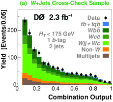
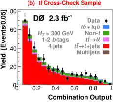
Figure 1: Combination discriminant in two cross-check samples.

The BDT analysis uses a common set of 64 discriminating variables for all analysis channels, but optimizes the filters separately in each channel. The BNN analysis selects 18–28 discriminating variables in each channel. The ME analysis uses only 2-jet and 3-jet events and splits the analysis into low-$H_{T}$ and high-$H_{T}$ regions at $H_{T}=175$ GeV. All three analyses transform their output distributions to ensure that every bin contains sufficient background statistics. We verify the agreement between data and background model for each multivariate method separate cross-check samples: a $W$+jets dominated sample and a $t\bar{t}$ dominated sample. The combination discriminant output for these two samples is shown in Fig. 1. Fig. 2 shows the combination discriminant output together with one of the discriminating variables for events in the signal region. The measured cross section is $\sigma_{tb+tqb}=3.94\pm 0.88{\rm~{}pb.}$ The measurement has a $p$-value of $2.6\times 10^{-7}$, corresponding to a significance of $5.0\,\sigma$.

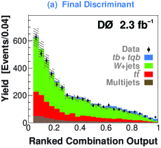
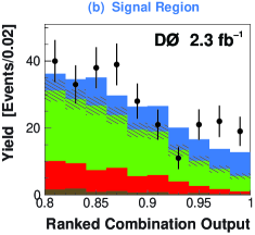
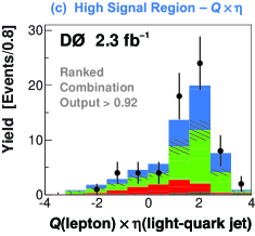
Figure 2: Combination discriminant for all analysis channels combined (a), only the signal region (b), and the pseudorapidity of the light quark jet multiplied by the lepton charge for events in the signal region (c). The signal is normalized to the measured cross section.

We use the cross section measurement to determine the Bayesian posterior for $|V_{tb}|^{2}$ in the interval [0,1] and extract a limit of $|V_{tb}|>0.78$ at 95% confidence level.

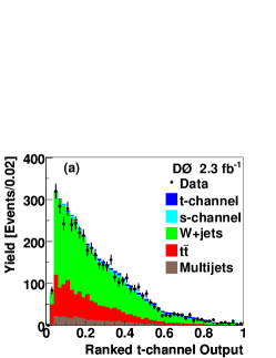
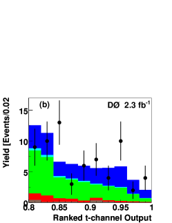
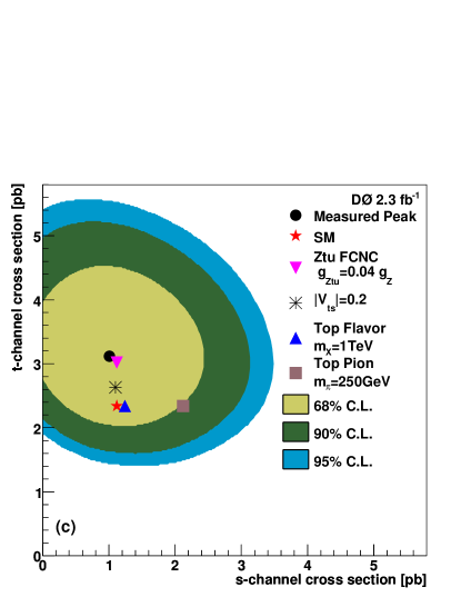
Figure 3: Ranked $t$-channel discriminant (a), only the signal region (b), and posterior probability density for $t$-channel and $s$-channel single top quark production (c). Also shown are the measured cross section, SM expectation, and several representative new physics scenarios [9, 28].

In a separate analysis we train the same multivariate methods using only $t$-channel single top events as signal and including SM $s$-channel in the background [27]. The $t$-channel discriminant output is shown in Figs. 3(a) and 3(b). We then determine the posterior as a function of both $s$-channel and $t$-channel as shown in Fig. 3(c). From this posterior we obtain the $t$-channel cross section by integrating over the $s$-channel axis and find $\sigma_{tqb}=3.14^{+0.94}_{-0.80}{\rm~{}pb.}$ We similarly extract the $s$-channel cross section as $\sigma_{tb}=1.05\pm 0.81$ pb by integrating over the $t$-channel axis. The observed p-value for the $t$-channel measurement is $8.0\times 10^{-7}$, corresponding to a Gaussian significance of $4.8\,\sigma$.

References

- [1] F. Abe et al. (CDF Collaboration), Phys. Rev. Lett. 74, 2626 (1995).
- [2] S. Abachi et al. (D0 Collaboration), Phys. Rev. Lett. 74, 2632 (1995).
- [3] G.V. Jikia and S.R. Slabospitsky, Phys. Lett. B 295, 136 (1992).
- [4] C.R. Chen, F. Larios, and C. P. Yuan, Phys. Lett. B 631, 126 (2005).
- [5] E. Boos, L. Dudko, and T. Ohl, Eur. Phys. J. C 11, 473 (1999)
- [6] A.P. Heinson, A.S. Belyaev, and E.E. Boos, Phys. Rev. D 56, 3114 (1997).
- [7] V.M. Abazov et al. (D0 Collaboration), Phys. Rev. Lett. 101, 221801 (2008).
- [8] V. M. Abazov et al. (D0 Collaboration), Phys. Rev. Lett. 102, 092002 (2009).
- [9] T. Tait and C.-P. Yuan, Phys. Rev. D 63, 014018 (2001).
- [10] V.M. Abazov et al. (D0 Collaboration), Phys. Rev. Lett. 98, 181802 (2007).
- [11] V.M. Abazov et al. (D0 Collaboration), Phys. Rev. D 78, 012005 (2008).
- [12] T. Aaltonen et al. (CDF Collaboration), Phys. Rev. Lett. 101, 252001 (2008).
- [13] V.M. Abazov et al. (D0 Collaboration), Phys. Rev. Lett. 103, 092001 (2009).
- [14] T. Aaltonen et al. (CDF Collaboration), Phys. Rev. Lett. 103, 092002 (2009).
- [15] N. Kidonakis, Phys. Rev. D 74, 114012 (2006).
- [16] V.M. Abazov et al. (D0 Collaboration), Nucl. Instrum. Methods Phys. Res. A 565, 463 (2006).
- [17] E. Boos et al., Phys. Atom. Nucl. 69, 1317 (2006); E. Boos et al. (CompHEP Collaboration), Nucl. Instrum. Methods Phys. Res. A 534, 250 (2004).
- [18] M.L. Mangano et al., JHEP 07, 001 (2003). We used alpgen version 2.05.
- [19] T. Sjöstrand et al., arXiv:hep-ph/0308153 (2003). We used pythia version 6.323.
- [20] L. Breiman et al., Classification and Regression Trees (Wadsworth, Stamford, 1984).
- [21] J.A. Benitez, Ph.D. thesis, Michigan State University, in preparation.
- [22] D. Gillberg, Ph.D. thesis, Simon Fraser University, FERMILAB-THESIS-2009-20 (2009).
- [23] R.M. Neal, Bayesian Learning for Neural Networks (Springer-Verlag, New York, 1996).
- [24] A. Tanasijczuk, Ph.D. thesis, Universidad de Buenos Aires, in preparation.
- [25] V.M. Abazov et al. (D0 Collaboration), Nature 429, 638 (2004).
- [26] M. Pangilinan, Ph.D. thesis, Brown University, in preparation.
- [27] V. M. Abazov et al. (D0 Collaboration), submitted to Phys. Lett. B, arXiv:0907.4259 (2009).
- [28] J. Alwall et al., Eur. Phys. J. C 49, 791 (2007).