We present non-extremal generalizations of $N_{f}=2N_{c}$ supergravity duals obtained by adding flavor branes to the Chamseddine-Volkov-Maldacena-Nuñez background and taking their backreaction into account. For a particular range of parameters we obtain a one parameter family of analytic black hole solutions with regular horizons. These solutions have a temperature that is always above the Hagedorn temperature of little string theory. We find that including flavor branes and their backreaction increases the minimum temperature of these systems from $T=\frac{1}{4\pi}$, for the background without flavor, to $T=\frac{1}{2\pi\sqrt{1+\epsilon}},\,\epsilon\ll 1$. We show that outside the range of validity of the analytic solutions presented here the backgrounds have naked singularities.

Hagedorn Systems from Backreacted Finite Temperature $N_{f}=2N_{c}$ Backgrounds

1 Introduction

The gauge/gravity duality ([1],[2],[3]) has proven to be a useful tool to study strongly coupled gauge theories. In the last few years finite temperature backgrounds have been used to explore strongly coupled plasmas yielding promising results. However, none of these non-extremal backgrounds includes matter in the fundamental representation other than in the quenched limit, for which $\frac{N_{f}}{N_{c}}\rightarrow 0$ as $N_{c}\rightarrow\infty$. Even at $T=0$ the issue of how to account for the backreaction of a large number of flavors is still being investigated. An important step in that directions was [4] where the authors presented a novel setup to include $N_{f}$ flavor branes, with $\frac{N_{f}}{N_{c}}\sim O(1)$, in the Chamseddine-Volkov-Maldacena-Nuñez (CVMN) model [5]. See also ([6]-[17]) for work that, using the techniques presented in [4], studies the inclusion of a large number of flavor branes in other backgrounds.
The CVMN background represents a large number of NS5 branes wrapped on a two-cycle of the resolved conifold. In the infrared it is dual to ${\mathcal{N}=1}\ \ SU(N)$ supersymmetric Yang-Mills in four dimensions. The ultraviolet completion is not a field theory but a little string theory ([18], [19]). The non-extremal deformation of CVMN was studied in [20]. It was shown to have Hagedorn behavior and to be thermodynamically unstable at high energies, behaving very much like finite temperature LST.
In [21] we found a one parameter family of solutions representing $N_{f}=2N_{c}$ flavor branes and their backreaction in the CVMN background. These solutions are conjectured to be dual to an ${\mathcal{N}}=1$ $SU(N)$ theory with $N_{f}=2N_{c}$ matter in the fundamental representation and some extra matter in the adjoint representation.
In the present note we find the non-extremal generalization of the solutions obtained in [21]. Our motivation is three-fold: 1)we want to investigate if turning on the temperature hides the singularity of the solutions presented in [21], 2) if that is the case, we want to understand if these backgrounds are good duals to finite temperature field theories or if they inherit the thermodynamical behavior of little string theory, 3) if they do behave like finite temperature LST, we want to understand what is the effect of the flavor branes and their backreaction.
For certain range of parameters we find a one parameter family of analytic solutions with regular horizons. The temperature of these solutions is $T\gtrsim\frac{1}{2\pi\sqrt{1+\epsilon}},\,\epsilon\ll 1$ indicating that its temperature is always above the Hagedorn temperature of LST which is $T=\frac{1}{4\pi}$. Outside the range of validity of our analytic solutions we have to perform a numerical study and find that the solutions have naked singularities. Hence, we conclude that our black hole solutions are not dual to a finite temperature field theory but to a little string theory with a temperature above the Hagedorn temperature.
Only few examples of supergravity backgrounds with Hagedorn behavior are known: NS5 branes and wrapped NS5 branes ([20], [23]). The thermal behavior of these examples has been thoroughly studied and it taught us several things about little string theory. We know that they are thermodynamically unstable and in [24] it was argued that the instability is of stringy origin. A different explanation was advocated in [25] where the authors argued that the instability was of supergravity origin, a Gregory-Lafflamme like instability. This issue, for the case of wrapped NS5 branes, was elucidated in [23] where it was shown that the instability is indeed of supergravity origin. We expect that our solutions will also be thermodynamically unstable, but further research is required to confirm this.

2 Black hole solutions

In this section we will review the metric ansatz considered in [20] which contains finite temperature solutions of the Chamseddine-Volkov-Maldacena-Nuñez (CVMN) background, [5]. It turns out that the metric ansatz is general enough to contain finite temperature generalizations of the more general supergravity backgrounds discussed in [4], [27], [28] and [21]. These more general supergravity backgrounds were found by adding a large number of smeared ’flavor’ D5 branes ($N_{f}\sim N_{c}$) to the CVMN background and taking their backreaction into account. They are conjectured to be dual to an $\mathcal{N}=1$ $SU(N_{c})$ gauge theory with $N_{f}$ quarks in the fundamental representation.
In the next subsections we derive the equations of motion for the fields for the special case of $\frac{N_{f}}{N_{c}}=2$ discussed in [21]. We find analytic solutions for black holes that have a horizon at large values of the radial coordinate and asymptote to the decoupled one parameter family of solutions discussed in [21]. Then we calculate the temperature for these solutions and argue that they are the only black holes within the validity of the supergravity approximation.

2.1 The metric ansatz and the equations of motion

The metric ansatz considered in [20] reads in Einstein frame

$$ds^{2} =-Y_{1}\,dt^{2}+Y_{2}\,d{\rm x}^{n}d{\rm x}^{n}+Y_{3}\,d\rho^{2}+Y_{4}\,(d\theta^{2}+\sin{\theta}^{2}d\varphi^{2})$$

$$+Y_{5}\,\left((w^{1}+Y_{7}d\theta)^{2}+(w^{2}-Y_{7}\sin\theta d\varphi)^{2}\right)+Y_{6}\,(w^{3}+\cos\theta d\varphi)^{2}\,,$$ (2.1)

where $Y_{i}=Y_{i}(\rho)$ and $w^{a}$ are the left-invariant one-forms on the $S^{3}$

$$w^{1} =\cos\psi d\tilde{\theta}+\sin\psi\sin\tilde{\theta}d\tilde{\varphi},$$

$$w^{2} =-\sin\psi d\tilde{\theta}+\cos\psi\sin\tilde{\theta}d\tilde{\varphi},$$ (2.2)

$$w^{3} =d\psi+\cos\tilde{\theta}d\tilde{\varphi}.$$

In addition we make the following ansatz for the RR 3-form $F_{3}$ [4]

$$F_{(3)} =\frac{N_{c}}{4}\Bigg{[}-(w^{1}+Y_{8}d\theta)\wedge(w^{2}-Y_{8}\sin\theta d\varphi)\wedge(w^{3}+\cos\theta d\varphi)$$

$$+Y_{8}^{\prime}dr\wedge(-d\theta\wedge w^{1}+\sin\theta d\varphi\wedge w^{2})+\left(1-Y_{8}^{2}-\frac{N_{f}}{N_{c}}\right)\sin\theta d\theta\wedge d\varphi\wedge w^{3}\Bigg{]}.$$ (2.3)

Note that $F_{3}$ is not closed due to the presence of the smeared flavor branes. Furthermore, we assume that the dilaton is also a function of $\rho$ and define $\phi=Y_{9}(\rho)$.
The complete action for type IIB supergravity with smeared flavor branes reads

$$S=S_{\text{grav}}+S_{\text{flavor}},$$ (2.4)

where, in Einstein frame, we have

$$S_{\text{grav}}=\frac{1}{2\kappa_{(10)}^{2}}\int d^{10}x\sqrt{-g_{(10)}}\left(R-\frac{1}{2}(\partial_{\mu}Y_{9})(\partial^{\mu}Y_{9})-\frac{1}{12}e^{Y_{9}}F_{(3)}^{2}\right),$$ (2.5)

and

$$S_{\text{flavor}}=\frac{T_{5}N_{f}}{4\pi^{2}}\left(-\int d^{10}x\sin\theta\sin\tilde{\theta}e^{Y_{9}/2}\sqrt{-g_{(6)}}+\int(\sin\theta\sin\tilde{\theta}d\theta\wedge d\varphi\wedge d\tilde{\theta}\wedge d\tilde{\varphi})\wedge C_{(6)}\right).$$ (2.6)

Plugging our ansätze into the action and integrating over all coordinates except $\rho$ and dropping the overall volume factor we a get a one-dimensional action with Lagrangian

$$L=\sum_{i,j}G_{ij}(Y)Y_{i}^{\prime}Y_{j}^{\prime}-U(Y)\equiv T-U.$$ (2.7)

We follow [20] and express the $Y_{i}$ in terms of nine other functions to make $G_{ij}$ diagonal

$$\begin{array}[]{ccc}Y_{1}=e^{2z-6x},&Y_{2}=e^{2z+2x},&Y_{3}=e^{10y-2z+2l},\\ Y_{4}=e^{2y-2z+2p+2q},&Y_{5}=e^{2y-2z+2p-2q},&Y_{6}=e^{2y-2z-8p},\\ Y_{7}=a,&Y_{8}=b,&Y_{9}=\phi.\end{array}$$ (2.8)

One finds that

$$T = e^{-l}\left(5y^{\prime 2}-3x^{\prime 2}-2z^{\prime 2}-5p^{\prime 2}-q^{\prime 2}-\frac{1}{4}\,e^{-4q}a^{\prime 2}-\frac{N_{c}^{2}}{64}\,e^{\phi+4z-4y-4p}b^{\prime 2}-\frac{1}{8}\phi^{\prime 2}\right)\,,$$

$$U = \frac{1}{8}\,e^{l}\bigg{[}e^{8y}\left\{e^{-12p}\,[e^{4q}+e^{-4q}(a^{2}-1)^{2}+2a^{2}(1-e^{10p-2q})^{2}]-8e^{-2p}\cosh\ 2q\right\}$$ (2.9)

$$+ \!\!\frac{N_{c}^{2}}{16}e^{\phi+4z+4y+4p}\!\left\{e^{4q}\!+e^{-4q}\!\left(\!a^{2}\!\!-\!2ab+\!1\!-\frac{N_{f}}{N_{c}}\!\right)^{2}\!\!\!+2(a\!-\!b)^{2}\!\right\}\!+\!N_{c}e^{\phi/2+2z+6y-4p}\bigg{]}.$$

Note that the $N_{c}$ dependence can be absorbed by shifting the dilaton, which we will do from now on. Since $l$ has no kinetic term, it is a pure gauge degree of freedom reflecting the remaining reparametrization invariance. Varying with respect to $l$ one can set it to any value. To make contact with the zero temperature solutions in [21], we want to have $b=0$ which implies $a=-\sqrt{1-e^{4q}}$.
The equation of motion for $x$ can be integrated once to get

$$x^{\prime}=-\frac{1}{4}e^{8f_{0}}d\,e^{l},$$ (2.10)

where the constant prefactor is chosen to simplify later expressions.
By comparing the equations of motion for $z$ and $\phi$ we find

$$\phi^{\prime}=4z^{\prime}+c_{\phi}e^{l}=4z^{\prime}+c_{x}x^{\prime},$$ (2.11)

where the constant $c_{x}=-\frac{4c_{\phi}}{e^{8f_{0}}d}$. We can integrate this to get

$$\phi=4z+c_{x}x,$$ (2.12)

where the integration constant can be set to zero by shifting the dilaton $\phi$. To make further contact with the solutions discussed in [21] we set $\frac{N_{f}}{N_{c}}=2$ and $l=-4(y+p-x)+\log{2}$. This leads to $Y_{6}=\frac{Y_{1}Y_{3}}{4Y_{2}}$. In the next section we solve the remaining equations to find analytic black hole solutions.

2.2 Black hole solutions

In this section we present analytical black hole solutions that asymptote to the decoupled one-parameter family described in [21]. To obtain these solutions we solve the remaining equations obtained from the Lagrangian (2.7) for large $\rho$. Note that from (2.1) and (2.8) we have that $Y_{1}/Y_{2}=e^{-8x}$. So in order to find black holes we need to solve for the deformation parameter $e^{8x}$ to all orders in the radial variable since we need $e^{8x}\rightarrow\infty$ at the horizon.
In order to obtain solutions that are regular at the horizon, we have to choose the constant in (2.12) such that $c_{x}=4$. To compare with the results of [21] we define

$$Y_{1}= e^{2f}e^{-8x},$$

$$Y_{2}= e^{2f},$$

$$Y_{3}= e^{2f}e^{2k}e^{8x},$$

$$Y_{4}= e^{2f}e^{2h},$$

$$Y_{5}= \frac{e^{2f}e^{2g}}{4},$$

$$Y_{6}= \frac{e^{2f}e^{2k}}{4},$$ (2.13)

where up to terms decaying more rapidly than $e^{-4\rho}$ we find

$$e^{h-g} =\frac{1}{2}-e^{-4\rho},$$

$$e^{h+g} =1+ce^{-\left(1+\sqrt{5}\right)\rho}+2e^{-4\rho},$$

$$e^{2k} =1-\left(1+\sqrt{5}\right)ce^{-\left(1+\sqrt{5}\right)\rho}-8e^{-4\rho},$$

$$e^{2f} =e^{2f_{0}+\frac{\rho}{2}}\left(1+\frac{1}{8}\left(-1+\sqrt{5}\right)ce^{-\left(1+\sqrt{5}\right)\rho}+\frac{1}{4}e^{-4\rho}\right),$$

$$e^{8x} =\frac{1}{1-8de^{-2\rho}}.$$ (2.14)

Here $c\,\epsilon\,\mathbb{R}$ is a free parameter distinguishing different solutions of the one-parameter family of decoupled solutions and $d$ corresponds to the temperature. For $d=0$ this reduces to a large $\rho$ expansion of the zero temperature solution found in [21]. For $d<0$ we see that $e^{8x}$ remains finite and there is no black hole. However, for $d>0$ we have a horizon at $\rho_{H}=\frac{\log{8d}}{2}$. Thus, for $d>0$, (2.2) is a family of black hole solutions representing the non-extremal deformation of the decoupled one parameter family of solutions presented in [21].

2.2.1 Restrictions on parameter space

To trust the analytic expression (2.2) we need to satisfy two conditions on $c$ and $d$. Since we neglected terms decaying faster than $e^{-4\rho}$ and want the analytic expression (2.2) to be valid all the way from the horizon $\rho_{H}$ to $\rho=\infty$ we need $\rho_{H}\gtrsim\frac{1}{4}$ i.e. $d\gtrsim\frac{\sqrt{e}}{8}$. Furthermore, we have to demand that $c$ is not too large so that the expansion for large $\rho$ is still valid. The most stringent constraint here comes from $e^{2k}$. We have to demand that $\left|\left(1+\sqrt{5}\right)ce^{-\left(1+\sqrt{5}\right)\rho_{H}}\right|\ll 1$ i.e., $|c|\ll\frac{(8d)^{\frac{1+\sqrt{5}}{2}}}{1+\sqrt{5}}$. There is another constraint on the possible values of $c$ and $d$ allowed. In [4] it was shown that the curvature blows up, if we approach the singularity where the flavor branes end. The value of the radial coordinate at which the Ricci scalar becomes large depends on $c$ and $d$. Calculating the Ricci scalar for our analytic solutions we find additional regions that are excluded because the curvature becomes large and the supergravity approximation breaks down. In particular the region with $d\lesssim 2$ is excluded. Figure 1 shows the allowed regions in the $(d,c)$ plane.

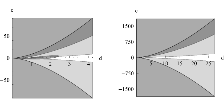
Figure 1: These plots show the $(d,c)$ plane. Our analytic black hole solutions are valid in the white region. The light gray region is excluded if we demand that $\left|(1+\sqrt{5})c(8d)^{-\frac{1+\sqrt{5}}{2}}\right|<.1$. The Ricci scalar is larger than 1 in the dark gray areas. The plots also show the curve $|c|=\frac{(8d)^{\frac{1+\sqrt{5}}{2}}}{1+\sqrt{5}}$.

2.2.2 Temperature

As long as these constraints on $c$ and $d$ are satisfied our analytic black hole solutions are valid. Calculating the black hole temperature observed at infinity we find

$$T =\frac{1}{4\pi}\left.\sqrt{\frac{Y_{1}}{(\rho-\rho_{H})^{2}Y_{3}}}\right|_{\rho=\rho_{H}}\left.\sqrt{\frac{Y_{3}}{Y_{1}}}\right|_{\rho=\infty}=\left.\frac{1}{2\pi\,e^{k}}\right|_{\rho=\rho_{H}}$$

$$=\frac{1}{2\pi\sqrt{1-\frac{\left(1+\sqrt{5}\right)c}{(8d)^{\frac{\left(1+\sqrt{5}\right)}{2}}}-\frac{1}{8d^{2}}}},$$ (2.15)

where we have used the fact that for the decoupled solutions $\left.\frac{Y_{3}}{Y_{1}}\right|_{\rho=\infty}=1$. From this expression we see that for $c\geq 0$ the temperature is always bigger than $T\geq\frac{1}{2\pi}$, which is obtained in the $d\rightarrow\infty$ limit. For $c<0$ we can do slightly better. If we set $\epsilon=-(1+\sqrt{5})c(8d)^{-\frac{1+\sqrt{5}}{2}}$, we find $T=\frac{1}{2\pi\sqrt{1+\epsilon-\frac{1}{8d^{2}}}}$. So for large $d$ we have $T\approx\frac{1}{2\pi\sqrt{1+\epsilon}}$ and we recall that we can trust our analytic solution only for $\epsilon\ll 1$. This should be compared with the result of [20] where the minimal temperature possible was the Hagedorn temperature of the little string theory $T=\frac{1}{4\pi}$. So we see that we have a similar situation and that at least for the analytic solutions the backreaction of the flavor branes has increased the minimal temperature we can have.

2.2.3 Beyond analytic solutions

We will now argue that there are no further black holes outside the regime of validity of our analytic solutions. First of all there are no black holes with a horizon at a small $\rho$ value. As we saw above and as was already noted in [21] the curvature becomes large for $\rho\gtrsim 1$ which is still within thse validity of our analytic solutions. We have numerically examined the other two regions with $|c|\gtrsim\frac{(8d)^{\frac{1+\sqrt{5}}{2}}}{1+\sqrt{5}}$ and the results agree with the expectations from the analytic solutions. One would generically expect that the solutions in these two regimes resemble the zero temperature results since the deformation parameter $d$ is relatively small compared to $c$. This is exactly what we find from the numerical solutions.
For $c\gtrsim\frac{(8d)^{\frac{1+\sqrt{5}}{2}}}{1+\sqrt{5}}$ one finds that $e^{2k}$ goes to zero and the curvature becomes large before we reach the horizon i.e., before $e^{8x}$ goes to infinity. This behavior could have been guessed from the expression for $e^{2k}$ in (2.2) and the figure 1. A representative plot of this behavior is shown in figure 2.

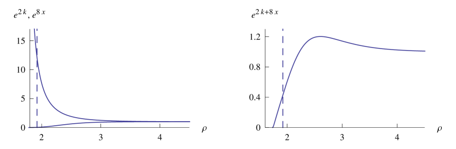
Figure 2: This plot shows numerical results for $e^{2k}$ and $e^{8x}$ for $d=10$ and $c=\frac{(8d)^{\frac{1+\sqrt{5}}{2}}}{1+\sqrt{5}}$. One sees on the left that coming from large $\rho$ $e^{2k}$ starts going towards zero at $\rho\approx 3$ while $e^{8x}$ starts to blow up. The right graph shows the product $e^{2k+8x}$ which goes to zero. The dashed line at $\rho_{c}\approx 1.92$ indicates where the Ricci scalar becomes large.

One sees that $e^{2k}$ becomes small and $e^{8x}$ starts to blow up for small $\rho$. The Ricci scalar also starts to blow up at $\rho_{c}\approx 1.92$ . One finds that $e^{2k(\rho_{c})}\approx 0.0356$ and $e^{8x(\rho_{c})}\approx 12.1$ and at $\rho_{f}\approx 1.74$ we have $e^{2k(\rho_{f})}\approx 2.60\times 10^{-15}$ and $e^{8x(\rho_{f})}\approx 134$. So as exemplified in the right graph in figure 2 we find that for $c\gtrsim\frac{(8d)^{\frac{1+\sqrt{5}}{2}}}{1+\sqrt{5}}$ the deformation $e^{8x}$ is subdominant and we do not have black holes in this regime.
For $c\lesssim-\frac{(8d)^{\frac{1+\sqrt{5}}{2}}}{1+\sqrt{5}}$ we find that $e^{2k}$ becomes very large and $e^{h+g}$ small. In figure 3 we plot the behavior of $e^{2k}$ and $e^{8x}$. We again find that the deformation $e^{8x}$ is subdominant.

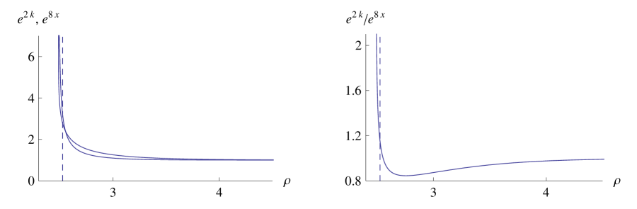
Figure 3: This plot shows the numerical results for $e^{2k}$ and $e^{8x}$ for $d=10$ and $c=-\frac{(8d)^{\frac{1+\sqrt{5}}{2}}}{1+\sqrt{5}}$. Both $e^{2k}$ and $e^{8x}$ become large in this regime as can be seen in the left graph. The right plot shows $e^{2k}/e^{8x}$ and one sees that $e^{8x}$ is subdominant to $e^{2k}$ for small $\rho$. The dashed line at $\rho_{c}\approx 2.53$ indicates where the Ricci scalar becomes large.

The behavior of $e^{2k}/e^{8x}$ in this regime is independent of the value of $d$ but it is interesting to study it as a function of $\epsilon=-(1+\sqrt{5})c(8d)^{-\frac{1+\sqrt{5}}{2}}$. One finds that $e^{8x}$ becomes dominant around $\epsilon\approx.2$ which might still be within the validity of our analytic solution which required $\epsilon\ll 1$.
So to summarize we find that outside the validity of our analytic solutions we have naked singularities. One might have expected this since the zero temperature solutions had those singularities and the deformation is small whenever the analytic solutions are not valid.

3 Conclusions

In previous work [21] we presented new supergravity backgrounds incorporating the backreaction of $N_{f}=2N_{c}$ flavor D5 branes in the CVMN background. In this note we find non-extremal generalizations of the solutions found in [21]. For a particular range of parameters we find a one parameter family of analytic solutions with a regular horizon. Outside the range of validity of these analytic solutions we show, numerically, that the solutions exhibit naked singularities.
The temperature of the regular solutions is always larger than the Hagedorn temperature of the LST. This is reminiscent of [20] where the non-extremal CVMN background -without flavor branes- was studied and a similar behavior was found. Thus, the solutions found here seem to be dual to a LST above its Hagedorn temperature rather than to a finite temperature $\mathcal{N}=1$ $SU(N_{c})$ gauge theory with a large number of fundamental matter.
We find that including flavor branes and their backreaction increases the minimal temperature from $T=\frac{1}{4\pi}$ [20], in the CVMN background without flavor, to $T=\frac{1}{2\pi\sqrt{1+\epsilon}},\,\epsilon\ll 1$ in the CVMN background with $N_{f}=2N_{c}$. Although our analysis is restricted to the special case $N_{f}=2N_{c}$ we believe that a similar conclusion can be reached for the more generic cases discussed in [4], [27], [28].
We believe that the one parameter family of Hagedorn systems presented here can contribute to our understanding of Little String Theory. In particular, a detailed study of the thermodynamics of these solutions and the possible existence of a tachyonic mode that can be identified with the thermodynamic instability ([29],[30]) are issues we think deserve further study.

4 Acknowledgments

We thank Matthias Ihl for collaboration at an initial stage of this work. E.C. thanks the Theory Group at the University of Texas at Austin, the Kavli Institute for Theoretical Physics and the Institute for Nuclear Physics at the University of Washington for hospitality as well as the Department of Energy for partial support during the completion of this work. E.C. and R.F. thank the Aspen Center for Physics for hospitality and partial support. The research of the authors is based upon work supported by the National Science Foundation under Grants No. PHY-0455649 and PHY05-51164. The research of E.C. is also funded by CONACYT grant 50760. The work of T.W. is also supported by the German Research Foundation (DFG) within the Emmy-Noether Programme (Grant number ZA 279/1-2).

References

- [1] J. M. Maldacena, “The large N limit of superconformal field theories and supergravity,” Adv. Theor. Math. Phys. 2, 231 (1998) [Int. J. Theor. Phys. 38, 1113 (1999)] [arXiv:hep-th/9711200].
- [2] S. S. Gubser, I. R. Klebanov and A. M. Polyakov, “Gauge theory correlators from non-critical string theory,” Phys. Lett. B 428, 105 (1998) [arXiv:hep-th/9802109].
- [3] E. Witten, “Anti-de Sitter space and holography,” Adv. Theor. Math. Phys. 2, 253 (1998) [arXiv:hep-th/9802150].
- [4] R. Casero, C. Nuñez and A. Paredes, “Towards the string dual of N = 1 SQCD-like theories,” Phys. Rev. D 73, 086005 (2006) [arXiv:hep-th/0602027].
-
[5]
J. M. Maldacena and C. Nuñez,
“Towards the large N limit of pure N = 1 super Yang Mills,”
Phys. Rev. Lett. 86, 588 (2001)
A. H. Chamseddine and M. S. Volkov, “Non-Abelian BPS monopoles in N = 4 gauged supergravity,” Phys. Rev. Lett. 79, 3343 (1997)
A. H. Chamseddine and M. S. Volkov, “Non-Abelian solitons in N = 4 gauged supergravity and leading order string theory,” Phys. Rev. D 57, 6242 (1998). - [6] F. Benini, F. Canoura, S. Cremonesi, C. Nuñez and A. V. Ramallo, “Unquenched flavors in the Klebanov-Witten model,” JHEP 0702, 090 (2007) [arXiv:hep-th/0612118].
- [7] F. Benini, F. Canoura, S. Cremonesi, C. Nuñez and A. V. Ramallo, “Backreacting Flavors in the Klebanov-Strassler Background,” JHEP 0709, 109 (2007) [arXiv:0706.1238 [hep-th]].
- [8] F. Canoura, P. Merlatti and A. V. Ramallo, “The supergravity dual of 3d supersymmetric gauge theories with unquenched flavors,” JHEP 0805, 011 (2008) [arXiv:0803.1475 [hep-th]].
- [9] F. Bigazzi, A. L. Cotrone and A. Paredes, “Klebanov-Witten theory with massive dynamical flavors,” arXiv:0807.0298 [hep-th].
- [10] F. Bigazzi, A. L. Cotrone, A. Paredes and A. V. Ramallo, “The Klebanov-Strassler model with massive dynamical flavors,” arXiv:0812.3399 [hep-th].
- [11] F. Bigazzi, A. L. Cotrone, A. Paredes and A. Ramallo, “Non chiral dynamical flavors and screening on the conifold,” arXiv:0810.5220 [hep-th].
- [12] D. Arean, P. Merlatti, C. Nuñez and A. V. Ramallo, “String duals of two-dimensional (4,4) supersymmetric gauge theories,” JHEP 0812, 054 (2008)
- [13] A. V. Ramallo, J. P. Shock and D. Zoakos, “Holographic flavor in N=4 gauge theories in 3d from wrapped branes,” JHEP 0902, 001 (2009)
- [14] J. Gaillard and J. Schmude, “On the geometry of string duals with backreacting flavors,” JHEP 0901, 079 (2009)
- [15] F. Bigazzi, A. L. Cotrone, A. Paredes and A. V. Ramallo, “Screening effects on meson masses from holography,” JHEP 0905, 034 (2009) [arXiv:0903.4747 [hep-th]].
- [16] O. C. Gurdogan, “Walking solutions in the string background dual to N=1 SQCD-like theories,” arXiv:0906.2429 [hep-th].
- [17] J. Gaillard and J. Schmude, “The lift of type IIA supergravity with D6 sources: M-theory with torsion,” arXiv:0908.0305 [hep-th].
- [18] M. Berkooz, M. Rozali and N. Seiberg, “Matrix description of M theory on T**4 and T**5,” Phys. Lett. B 408, 105 (1997) [arXiv:hep-th/9704089].
- [19] N. Seiberg, “New theories in six dimensions and matrix description of M-theory on T**5 and T**5/Z(2),” Phys. Lett. B 408, 98 (1997) [arXiv:hep-th/9705221].
- [20] S. S. Gubser, A. A. Tseytlin and M. S. Volkov, “Non-Abelian 4-d black holes, wrapped 5-branes, and their dual descriptions,” JHEP 0109, 017 (2001) [arXiv:hep-th/0108205].
- [21] E. Cáceres, R. Flauger, M. Ihl and T. Wrase, “New Supergravity Backgrounds Dual to N=1 SQCD-like Theories with ,” JHEP 0803, 020 (2008) [arXiv:0711.4878 [hep-th]].
- [22] E. Caceres, R. Flauger, M. Ihl and T. Wrase, “Backreaction And N(F) = 2n(C) Sqcd-Like Theories,” AIP Conf. Proc. 1116, 301 (2009).
- [23] A. Buchel, “On the thermodynamic instability of LST,” arXiv:hep-th/0107102.
- [24] D. Kutasov and D. A. Sahakyan, “Comments on the thermodynamics of little string theory,” JHEP 0102, 021 (2001) [arXiv:hep-th/0012258].
- [25] M. Rangamani, “Little string thermodynamics,” JHEP 0106, 042 (2001) [arXiv:hep-th/0104125].
- [26] G. Bertoldi and C. Hoyos-Badajoz, “Stability of linear dilaton black holes at the Hagedorn temperature,” arXiv:0903.3431 [hep-th].
- [27] R. Casero, C. Nuñez and A. Paredes, “Elaborations on the String Dual to N=1 SQCD,” Phys. Rev. D 77, 046003 (2008) [arXiv:0709.3421 [hep-th]].
- [28] C. Hoyos-Badajoz, C. Nuñez and I. Papadimitriou, “Comments on the String dual to N=1 SQCD,” arXiv:0807.3039 [hep-th].
- [29] S. S. Gubser and I. Mitra, “Instability of charged black holes in anti-de Sitter space,” arXiv:hep-th/0009126.
- [30] A. Buchel, “A holographic perspective on Gubser-Mitra conjecture,” Nucl. Phys. B 731, 109 (2005) [arXiv:hep-th/0507275].