Pressure-induced diamond to $\beta$-tin transition in bulk silicon:
a near-exact quantum Monte Carlo study

Abstract

The pressure-induced structural phase transition from diamond to $\beta$-tin in silicon is an excellent test for theoretical total energy methods. The transition pressure provides a sensitive measure of small relative energy changes between the two phases (one a semiconductor and the other a semimetal). Experimentally, the transition pressure is well characterized. Density-functional results have been unsatisfactory. Even the generally much more accurate diffusion Monte Carlo method has shown a noticeable fixed-node error. We use the recently developed phaseless auxiliary-field quantum Monte Carlo (AFQMC) method to calculate the relative energy differences in the two phases. In this method, all but the error due to the phaseless constraint can be controlled systematically and driven to zero. In both structural phases we were able to benchmark the error of the phaseless constraint by carrying out exact unconstrained AFQMC calculations for small supercells. Comparison between the two shows that the systematic error in the absolute total energies due to the phaseless constraint is well within 0.5m$E_{\textrm{h}}$/atom. Consistent with these internal benchmarks, the transition pressure obtained by the phaseless AFQMC from large supercells is in very good agreement with experiment.

I Introduction

Theoretical and computational treatment of the effects of electron correlations remains a significant challenge. Despite decades of effort invested into solving the Schroedinger equation (by independent-particle, mean-field and perturbative methods), there are still major difficulties in predicting and explaining many phenomena related to bonding, cohesion, optical properties, magnetic orderings, superconductivity and other quantum effects. The pressure-induced structural phase transition in silicon from diamond to $\beta$-tin Mujica et al. (2003) is an excellent test for theoretical total energy methods. The transition pressure provides a sensitive measure of small relative energy changes between the two phases (one a semiconductor and the other a semimetal). Experimentally, the transition pressure is well characterized. Density-functional theory (DFT) results have been unsatisfactory, exhibiting sensitivity to the particular form of the exchange-correlation (xc) functional. Even the generally much more accurate diffusion Monte Carlo (DMC) method Moskowitz et al. (1982); P. J. Reynolds, D. M. Ceperley, B. J. Alder and W. A. Lester, Jr. (1982); Foulkes et al. (2001); Hammond et al. (1994); Kalos and Whitlock (1986) has shown Alfè et al. (2004) a noticeable fixed-node J. B. Anderson (1976) error.

The phaseless auxiliary-field (AF) quantum Monte Carlo (QMC) AFQMC method Zhang and Krakauer (2003); Al-Saidi et al. (2006a); Suewattana et al. (2007a) provides a new alternative for ab initio many-body calculations to address electron correlation effects. All stochastic QMC methods Ceperley and Alder (1980); Reynolds et al. (1982); Foulkes et al. (2001); Zhang and Krakauer (2003) use projection from a reference many-body wave function. In principle these methods are exact. In practice, however, the fermionic sign problem Ceperley and Alder (1984); Zhang and Kalos (1991); Zhang (1999); Foulkes et al. (2001); Zhang and Krakauer (2003) causes exponential growth of the variance with system size and projection time. Transient methods, Ceperley and Alder (1980); Rom et al. (1997); Baer et al. (1998) which maintain exactness while enduring the sign problem, can be very useful if sufficiently accurate information can be obtained with a relatively short projection, as we illustrate in the present paper (Sec. IV.1). In general, however, the sign problem must be completely eliminated (usually with an approximation) to achieve a general, efficient method for realistic systems. The majority of QMC calculations in fermion systems have been done in this form, for example with the fixed-node approximation J. B. Anderson (1976); Foulkes et al. (2001) in DMC, which has been the most commonly applied QMC method in electronic structure.

The phaseless AFQMC controls the sign problem with a global phase condition in the over-complete manifold of Slater determinants (in which antisymmetry is imposed). Since the antisymmetry ensures that each walker is automatically “fermionic”, the tendency for the walker population to collapse to a global bosonic state is eliminated in this approach. It is reasonable to expect that an overall phase constraint applied in this manifold to be less restrictiveZhang (1999). Applications indicate that this often is the case. In a variety of systems AFQMC has demonstrated accuracy equaling or surpassing the most accurate (non-exponential scaling) many-body computational methods. These include first- and second-row molecules, Al-Saidi et al. (2006a); Zhang et al. (2005) transition metal oxide molecules, Al-Saidi et al. (2006b) simple solids, Zhang and Krakauer (2003); Kwee et al. (2008a) post-$d$ elements Al-Saidi et al. (2006c) van der Waals systems, Al-Saidi et al. (2007a) molecular excited states, Purwanto et al. (2009) and in molecules in which bonds are being stretched or broken. Al-Saidi et al. (2007b); Purwanto et al. (2008, 2009) Most of these calculations used a mean-field single determinant taken directly from DFT or Hartree-Fock (HF) for the trial wave function in the phaseless constraint. As a result, the phaseless AFQMC method reduces the reliance of QMC on the quality of the trial wave function. Al-Saidi et al. (2006a, 2007b); Purwanto et al. (2008) This is desirable in order to make QMC more of a general and “blackbox” approach.

The use of a basis set is a second feature that distinguishes the AFQMC method from the standard DMC method. Moskowitz et al. (1982); P. J. Reynolds, D. M. Ceperley, B. J. Alder and W. A. Lester, Jr. (1982); Foulkes et al. (2001); Hammond et al. (1994); Kalos and Whitlock (1986) The latter works in electron coordinate space. As a result, there is no finite basis set error per se in DMC. There are presently two main flavors of the phaseless AFQMC method, corresponding to two different choices of the one-electron basis: (i) planewave with norm-conserving pseudopotential (as widely adopted in solid state physics), Zhang and Krakauer (2003); Suewattana et al. (2007a) and (ii) Gaussian type basis sets (the standard in quantum chemistry). Al-Saidi et al. (2006a) In planewave AFQMC, convergence to the basis set limit is easily controlled, as in DFT calculations, using the plane wave cutoff energy $E_{\mathrm{cut}}$.

In this paper, planewave AFQMC is used to calculate the relative energy differences between the two phases. The goal is to examine the accuracy of phaseless AFQMC, benchmarking the energy difference at the transition volumes against experiment and DMC results, and against exact free-projection AFQMC using smaller primitive cells. In the phaseless AFQMC approach, all but the error from the phaseless constraint can be controlled systematically and driven essentially to zero. Comparison with exact AFQMC free-projection shows that the systematic error in the total energies due to the phaseless constraint is well within 0.5m$E_{\textrm{h}}$/atom. Consistent with these internal benchmarks, the transition pressure calculated from the phaseless AFQMC in large supercells is found to be in very good agreement with experiment.

The paper is organized as follows. Several aspects of the AFQMC method, including the hybrid formulation and the reduction of weight fluctuation, are described in Sec. II. This is followed by specific planewave AFQMC calculational details in Sec. III. Calculated results are presented and discussed in Sec. IV. Finally, we summarize and conclude in Sec. V.

II AFQMC methodology

This section reviews aspects of the AFQMC method in some detail. This is done to facilitate the discussion of systematic errors in Secs. III and IV, and to provide additional details on some phaseless AFQMC variants which are used in this paper. More complete descriptions of the phaseless AFQMC method can be found in Refs. Zhang and Krakauer, 2003; Purwanto and Zhang, 2004, 2005; Al-Saidi et al., 2006a; Suewattana et al., 2007a.

II.1 AFQMC projection by random walks

The ground state of a many-body system, $|{{\Psi_{0}}}\rangle$, is obtained by means of iterative projection from a trial wave function $|{{\Psi_{\mathrm{T}}}}\rangle$:

$$\begin{split}e^{-\tau{\hat{H}}}e^{-\tau{\hat{H}}}\cdots e^{-\tau{\hat{H}}}|{{\Psi_{\mathrm{T}}}}\rangle\rightarrow|{{\Psi_{0}}}\rangle\,,\end{split}$$ (1)

where ${\hat{H}}={\hat{K}}+{\hat{V}}$ is the Hamiltonian of the system, consisting of all one-body terms, ${\hat{K}}$, and two-body terms, ${\hat{V}}$. AFQMC implements the ground-state projection as random walks in the space of Slater determinants. The Trotter-Suzuki breakup

$$\begin{split}e^{-\tau{\hat{H}}}=e^{-\tau{\hat{K}}/2}e^{-\tau{\hat{V}}}e^{-\tau{\hat{K}}/2}+\mathcal{O}\left(\tau^{3}\right)\end{split}$$ (2)

is used to separate the one- and two-body terms. Expressing ${\hat{V}}$ as a sum of the squares of one-body operators $\{{\hat{v}}_{i}\}\equiv{\hat{\mathbf{v}}}$:

$$\begin{split}{\hat{V}}=-\frac{1}{2}\sum_{i}{\hat{v}}_{i}^{2}=-\frac{1}{2}{\hat{\mathbf{v}}}\cdot{\hat{\mathbf{v}}}\,,\end{split}$$ (3)

the Hubbard-Stratonovich (HS) transformation Stratonovich (1957); Hubbard (1959) is then used to express the two-body projector as a multidimensional integral

$$\begin{split}e^{-\tau{\hat{V}}}=\prod_{i}\int_{-\infty}^{\infty}\frac{d\sigma_{i}}{\sqrt{2\pi}}e^{-\sigma_{i}^{2}/2}e^{\sqrt{\tau}\,\sigma_{i}{\hat{v}}_{i}}\,.\end{split}$$ (4)

Using Eq. (4) effectively maps the two-body interaction onto a fictitious non-interacting Hamiltonian with coupling to auxiliary classical fields $\{{\sigma}_{i}\}\equiv\bm{\sigma}$. The operation of the one-body projector on a Slater determinant $|{{\phi}}\rangle$ simply yields another determinant: $|{{\phi^{\prime}}}\rangle=e^{\sqrt{\tau}\,\bm{\sigma}\cdot{\hat{\mathbf{v}}}}|{{\phi}}\rangle$. If $|{{\Psi_{\mathrm{T}}}}\rangle$ in Eq. (1) is expressed as a sum of Slater determinants (e.g., just one if $|{{\Psi_{\mathrm{T}}}}\rangle$ is a HF or DFT solution), the integral in Eq. (4) can then be evaluated using Monte Carlo sampling over random walker streams. Zhang et al. (1997); Zhang and Krakauer (2003)

As discussed further in Sec. II.2, it is advantageous computationally to rewrite the two-body potential in Eq. (3), subtracting the mean-field contribution Rom et al. (1997); Baer et al. (1998); Purwanto and Zhang (2005); Al-Saidi et al. (2006d) prior to the HS transformation:

$$\begin{split}{\hat{V}}&=-\left[\frac{1}{2}({\hat{\mathbf{v}}}-\bar{\mathbf{v}}_{\textrm{mf}})^{2}+{\hat{\mathbf{v}}}\cdot\bar{\mathbf{v}}_{\textrm{mf}}-\frac{1}{2}\bar{\mathbf{v}}_{\textrm{mf}}^{2}\right]\,,\end{split}$$ (5)

where $\bar{\mathbf{v}}_{\textrm{mf}}$ is generally chosen to be the expectation value of the ${\hat{\mathbf{v}}}$ operator with respect to the trial wave function

$$\begin{split}\bar{\mathbf{v}}_{\textrm{mf}}\equiv\frac{\langle{{\Psi_{\mathrm{T}}}}|{{{\hat{\mathbf{v}}}}}|{{\Psi_{\mathrm{T}}}}\rangle}{\langle{{\Psi_{\mathrm{T}}}}|{{\Psi_{\mathrm{T}}}}\rangle}\,.\end{split}$$ (6)

II.2 Phaseless AFQMC

In principle, the procedure in Eqs. (1-4) yields the exact ground state. The basic idea can be efficiently realized by branching random walks, as is used in Sec. IV.1 to carry out exact free-projection. In practice, however, a phase problem appears, because the repulsive Coulomb interaction gives rise to imaginary ${\hat{\mathbf{v}}}$, complex walkers $|{{\phi}}\rangle$, and complex $\langle{{\Psi_{\mathrm{T}}}}|{{\phi}}\rangle$ overlaps, causing the variance to grow exponentially and swamp the signal. To control this problem, importance sampling and a phaseless approximationZhang and Krakauer (2003) were introduced, yielding a stable stochastic simulation. The importance sampling transformation leads to a representation of the ground-state wave function as a weighted sum of Slater determinants $\{|{{\phi}}\rangle\}$: Zhang and Krakauer (2003); Purwanto and Zhang (2004)

$$\begin{split}|{{\Psi_{0}}}\rangle=\sum_{\phi}w_{\phi}\frac{|{{\phi}}\rangle}{\langle{{\Psi_{\mathrm{T}}}}|{{\phi}}\rangle}\,.\end{split}$$ (7)

A force bias term results in Eq. (4):

$$\begin{split}e^{-\tau{\hat{V}}}=\prod_{i}\int_{\infty}^{\infty}\frac{d\sigma_{i}}{\sqrt{2\pi}}e^{-\sigma_{i}^{2}/2}e^{\sigma_{i}\bar{\sigma}_{i}-\bar{\sigma}_{i}^{2}/2}e^{\sqrt{\tau}\,(\sigma_{i}-\bar{\sigma}_{i}){\hat{v}}_{i}}\,.\end{split}$$ (8)

The corresponding importance-sampled one-body propagator then takes the form

$$\begin{split}w_{\phi^{\prime}}|{{\phi^{\prime}}}\rangle\leftarrow\left[\int d\bm{\sigma}g(\bm{\sigma}){\hat{B}}(\bm{\sigma}-\bar{\bm{\sigma}})W(\bm{\sigma},\bar{\bm{\sigma}})\right]w_{\phi}|{{\phi}}\rangle\,,\end{split}$$ (9)

where $\{\bar{\sigma}_{i}\}\equiv\bar{\bm{\sigma}}$, $g(\bm{\sigma})$ is the multidimensional Gaussian probability density function with zero mean and unit width, and

$${\hat{B}}(\bm{\sigma}-\bar{\bm{\sigma}}) \equiv e^{-\tau{\hat{K}}/2}e^{\sqrt{\tau}\,(\bm{\sigma}-\bar{\bm{\sigma}})\cdot{\hat{\mathbf{v}}}}e^{-\tau{\hat{K}}/2}\,,$$ (10)

$$|{{\phi^{\prime}}}\rangle ={\hat{B}}(\bm{\sigma}-\bar{\bm{\sigma}})\,|{{\phi}}\rangle\,,$$ (11)

$$W(\bm{\sigma},\bar{\bm{\sigma}}) \equiv\frac{\langle{{\Psi_{\mathrm{T}}}}|{{{\hat{B}}(\bm{\sigma}-\bar{\bm{\sigma}})}}|{{\phi}}\rangle}{\langle{{\Psi_{\mathrm{T}}}}|{{\phi}}\rangle}e^{\bm{\sigma}\cdot\bar{\bm{\sigma}}-\bar{\bm{\sigma}}\cdot\bar{\bm{\sigma}}/2}\,.$$ (12)

The one-body operator ${\hat{B}}$ generates the random walker stream, transforming $|{{\phi}}\rangle$ into $|{{\phi^{\prime}}}\rangle$, while $W$ updates the weight factor $w_{\phi}$.

The optimal choice of $\bar{\bm{\sigma}}$, which cancels the weight fluctuation to $\mathcal{O}\left(\sqrt{\tau}\right)$, is given by

$$\begin{split}\bar{\bm{\sigma}}=-\sqrt{\tau}\,\frac{\langle{{\Psi_{\mathrm{T}}}}|{{{\hat{\mathbf{v}}}}}|{{\phi}}\rangle}{\langle{{\Psi_{\mathrm{T}}}}|{{\phi}}\rangle}\,,\end{split}$$ (13)

where $\phi$ is the determinant being propagated. Using this choice, the weight update factor $W$ can be written as Zhang and Krakauer (2003)

$$\begin{split}W(\bm{\sigma},\bar{\bm{\sigma}})\approx e^{-\tau{\langle{{\Psi_{\mathrm{T}}}}|{{{\hat{H}}}}|{{\phi}}\rangle}/{\langle{{\Psi_{\mathrm{T}}}}|{{\phi}}\rangle}}\equiv e^{-\tau E_{\mathrm{L}}[\phi]}\,,\end{split}$$ (14)

where $E_{\mathrm{L}}[\phi]$ is referred to as the “local energy” of $|\phi\rangle$. In practice, we use the average of two local energies to update the weight:

$$\begin{split}W(\bm{\sigma},\bar{\bm{\sigma}})\approx e^{-\tau(E_{\mathrm{L}}[\phi^{\prime}]+E_{\mathrm{L}}[\phi])/2}\,.\end{split}$$ (15)

The total energy can be calculated using the mixed-estimate form, which is not variational Zhang and Krakauer (2003).

The key to controlling the phase problem is to prevent a two-dimensional random walk in the complex $\langle{{\Psi_{\mathrm{T}}}}|{{\phi}}\rangle$-plane, thus avoiding the growth of a finite density at the origin. To do this, the phase rotation of the walker $|{{\phi}}\rangle$ is defined by

$$\begin{split}\Delta\theta\equiv\arg\left(\frac{\langle{{\Psi_{\mathrm{T}}}}|{{\phi^{\prime}}}\rangle}{\langle{{\Psi_{\mathrm{T}}}}|{{\phi}}\rangle}\right)\,,\end{split}$$ (16)

and the walker weight is “projected” to its real, positive value:

$$\begin{split}w_{\phi^{\prime}}\leftarrow\begin{cases}\cos(\Delta\theta)\,|W(\bm{\sigma},\bar{\bm{\sigma}})|\,w_{\phi}\,,&|\Delta\theta|<\pi/2\\ 0\,,&\textrm{otherwise}\end{cases}\,.\end{split}$$ (17)

If the mean-field background is non-zero, its subtraction in Eq. (5) can lead to a reduction in the average rotation angle $\Delta\theta$ (and variance of the energy). Purwanto and Zhang (2005); Al-Saidi et al. (2006d)

II.3 AFQMC in hybrid form

Most applications to date have used the phaseless AFQMC local energy formalism, described above. In planewave AFQMC, evaluating $E_{\mathrm{L}}$ scales as $\mathcal{O}\left(N^{2}M\log M\right)$, while the propagation step [Eq. (9)] scales as $\mathcal{O}\left(NM\log M\right)$, using fast Fourier transforms.Suewattana et al. (2007b) Computation of the overlap matrix and other operations scale no worse than $\mathcal{O}\left(N^{2}M\right)$.

To reduce the frequency of evaluating $E_{\mathrm{L}}$, the most costly part of the calculation, we can use an alternative formulation, the “hybrid” form Zhang and Krakauer (2003); Purwanto and Zhang (2004) of the walker weight in Eq. (12). In the hybrid variant, only measurement evaluations of $E_{\mathrm{L}}$ are needed. Since the autocorrelation time is typically $50$-$100$ times the time step $\tau$, this variant may be more efficient. The hybrid method tends to have larger variance than the local energy method, however. The latter satistifies zero-variance in the limit of an exact $|\Psi_{T}\rangle$, explicitly canceling out some $\mathcal{O}\left(\tau\right)$ terms. The two methods also have different Trotter behaviors, as illustrated in Sec. III.2, but they approach the same answer as $\tau\to 0$. The hybrid method is used for the large supercell calculations reported in this paper.

II.4 Random walk bounds: controlling rare event fluctuations

For any finite population of walkers, the stochastic nature of the simulation does not preclude rare events, which cause extremely large population fluctuations. For example, a walker near the origin of the $\langle{{\Psi_{\mathrm{T}}}}|{{\phi}}\rangle$-plane can acquire a very large weight in a move $|\phi^{\prime}\rangle\leftarrow{\hat{B}}|\phi\rangle$ [Eq. (9)], due to the occurence of a very large $\langle{{\Psi_{\mathrm{T}}}}|{{\phi^{\prime}}}\rangle/\langle{{\Psi_{\mathrm{T}}}}|{{\phi}}\rangle$ ratio [Eq. (12) or Eq. (14)]. To circumvent the problem in a simulation of finite population, we apply a bound condition in the local energy method:

$$\begin{split}(E_{L}^{0}-\Delta E_{\mathrm{L}})\leq E_{\mathrm{L}}[\phi]\leq(E_{L}^{0}+\Delta E_{\mathrm{L}}),\end{split}$$ (18)

where the width of the energy range $\Delta E_{L}$ is defined as

$$\begin{split}\Delta E_{\mathrm{L}}\equiv\sqrt{\frac{2}{\tau}}\,,\end{split}$$ (19)

and where the average local energy value $E_{L}^{0}$ is obtained by averaging $E_{\mathrm{L}}$ measurements during the growth phase.Zhang et al. (1997) If $E_{\mathrm{L}}$ goes outside this range, it is capped at the maximum or minimum of the range. For a typical $\tau$ ($\sim 0.05E_{\textrm{h}}^{-1}$), the energy range allowed by Eq. (18) is large ($\sim 12E_{\textrm{h}}$), so $E_{\mathrm{L}}$ is capped only in very rare instances.

Similar bounds are introduced in the hybrid AFQMC method. Defining the hybrid energy as [compare Eqs. (12] and (14]

$$\begin{split}E_{\mathrm{H}}[\phi]&\equiv-\frac{\log W(\bm{\sigma},\bar{\bm{\sigma}})}{\tau}\\ &=-\frac{1}{\tau}\left[\log\left(\frac{\langle{{\Psi_{\mathrm{T}}}}|{{{\hat{B}}(\bm{\sigma}-\bar{\bm{\sigma}})}}|{{\phi}}\rangle}{\langle{{\Psi_{\mathrm{T}}}}|{{\phi}}\rangle}\right)+\bm{\sigma}\cdot\bar{\bm{\sigma}}-\frac{1}{2}\bar{\bm{\sigma}}\cdot\bar{\bm{\sigma}}\right]\,,\end{split}$$ (20)

the value of $E_{\mathrm{H}}$ is bounded as

$$\begin{split}(E_{H}^{0}-\Delta E_{\mathrm{H}})\leq E_{\mathrm{H}}[\phi]\leq(E_{H}^{0}+\Delta E_{\mathrm{H}})\,,\end{split}$$ (21)

where $E_{H}^{0}$ is estimated as in Eq. (18).

In addition, the walker weights are also bounded such that $w_{\phi}\leq w_{\max}$ at all times for a reasonable $w_{\max}$ (typically set to the smaller of $100$ or $0.1$ times the size of the population). This bound is rarely triggered when the $E_{\mathrm{H}}$ or $E_{\mathrm{L}}$ bounding scheme is in place.

Finally, a force-bias bound is applied in both the local energy and hybrid methods. This prevents large modification of the orbitals when the denominator $\langle{{\Psi_{\mathrm{T}}}}|{{\phi}}\rangle$ in Eq. (13) is small:

$$\begin{split}|\bar{\sigma}_{i}|\leq 1.0.\end{split}$$ (22)

This bound is implicitly $\tau$-dependent, as seen in Eq. (13). We have found that the energy cap ($E_{\mathrm{L}}$ or $E_{\mathrm{H}}$) had the most effect in controlling weight fluctuations.

It is important to note that the bounds being applied, while ad hoc, have well-defined limiting behavior. As $\tau\to 0$, the bounds on the physical quantities $E_{L}$ and $\langle{\hat{v}}\rangle$ both approach $\infty$. The bounds only affect the Trotter error at finite $\tau$, but not the final answer when $\tau$ is extrapolated to zero.

II.5 Exact calculations: unconstrained AFQMC

To estimate the accuracy of phaseless AFQMC, calculations using exact unconstrained “free” projection were carried out (Sec. III). In free projection, the weights $\{w_{\phi}\}$ are allowed to acquire a phase. This is implemented using a modified form of the hybrid method, where the mean-field average of the ${\hat{\mathbf{v}}}$ operators is used as the force bias [instead of Eq. (13)],

$$\begin{split}\bar{\bm{\sigma}}_{\textrm{mf}}&=-\sqrt{\tau}\,\bar{\mathbf{v}}_{\textrm{mf}}\,.\end{split}$$ (23)

This choice is equivalent to the subtraction of mean-field contribution to the two-body potential described in Eq. (5). The use of the mean-field background subtraction is essential in prolonging the stability of the simulation before the signal is lost to the phase problem. None of the bounds in the preceding subsection is applied in the free-projection calculations.

III AFQMC computational details for silicon diamond and $\beta$-tin

The present calculations are carried out with planewave based AFQMC (PW-AFQMC), which uses norm-conserving and separable Kleinman-Bylander Kleinman and Bylander (1982) pseudopotentials to achieve efficient $\mathcal{O}\left(N^{2}M\log M\right)$ system size scaling, similar to planewave based DFT (PW-DFT) calculations. We first describe specific computational details of the planewave AFQMC calculations, including the pseudopotential, planewave cutoff, and supercells.

Convergence to the basis set limit is easily controlled, as in DFT calculations, using the plane wave cutoff energy $E_{\mathrm{cut}}$. Our calculations used $E_{\mathrm{cut}}=12.5E_{\textrm{h}}$, which is the design cutoff of our Si pseudopotential (see below). For material systems such as silicon, we have previously shown Suewattana et al. (2007a) that a good $E_{\mathrm{cut}}$ at the DFT level, as determined by the norm-conserving pseudopotential, is sufficient to converge the two-particle correlations in AFQMC to within typical ststistical errors. In DFT calculations with the local density approximation (LDA), the total absolute energies of the diamond primitive cell using this $E_{\mathrm{cut}}$ has an error of $\simeq 0.43\,\textrm{m}E_{\textrm{h}}$ (as verified by using increasingly larger values of $E_{\mathrm{cut}}$). Basis set convergence errors of energy differences are much smaller, of course.

AFQMC calculations for large 54-atom $3\times 3\times 3$ diamond and $\beta$-tin supercells were done to obtain the transition pressures, after finite-size corrections, discussed below. Test calculations, such as pseudopotential tests and comparisons with benchmark exact AFQMC, were carried out for the smaller 2-atom primitive unit cells.

For each supercell and $\mathbf{k}$-point, corresponding trial wave functions $|{{\Psi_{\mathrm{T}}}}\rangle$ were taken as generated from DFT-LDA, using the ABINIT code Gonze et al. (2002). In $\beta$-tin, random $\mathbf{k}$ points are used, rather than special points such as Monkhorst Pack sets, to remove open-shell effects. For each $\mathbf{k}$, our single-determinant trial wave function is thus unique and non-degenerate at the “Fermi surface.”

In the following subsections, aspects of the Si OPIUM pseudopotential are first discussed. The quality of the pseudopotential is assessed by comparing the equation of state (EOS) for the diamond and $\beta$-tin structures with all-electron results within the framework of DFT. Next, efficient finite-size corrections are described, separately analyzing one-body errors, which are analogous to $\mathbf{k}$ sampling in PW-DFT, and two-body Coulomb finite size errors.

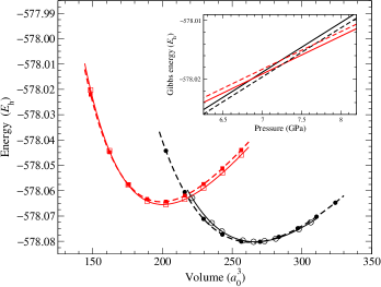
Figure 1: (Color online) Equation of state for the Si diamond and $\beta$-tin phases, comparing all-electron (solid lines) and pseudopotential (dashed lines) DFT-LDA results. The inset shows the Gibbs energy as a function of the pressure.

Table 1: Quantities of the diamond and $\beta$-tin phases of silicon computed with DFT, using all-electron LAPW and planewave pseudopotential methods. The xc functional used is the Perdew-Wang LDA. Volumes and lattice constants are expressed in atomic units ($a_{0}^{3}$ and $a_{0}$, respectively); energies are in eV; bulk moduli and pressures are in GPa.

Quantity	Pseudopotential	LAPW
diamond phase
Equilibrium volume	263.888	266.474
Equilibrium lattice constant	10.182	10.215
Bulk modulus	95.380	95.327
Cohesive energy	5.413	5.409
$\beta$-tin phase
Equilibrium volume	199.132	200.364
Bulk modulus	114.760	114.947
Transition pressure	7.67	6.86

III.1 Si pseudopotential quality

The optimized design method Rappe et al. (1990) was used to generate the Si pseudopotenital with OPIUM. OPI The atomic reference state was [Ne] 3s² 3p^1.5 3d^0.4. All angular momentum channels ($l=0,1,2$) used a cutoff radius $r_{c}=2.08$ Bohr, with $l=2$ as the local potential. The optimized design pseudo-wavefunction was expanded using five spherical Bessel functions with wave vector $q_{c}=5.0~{}\mathrm{Bohr}^{-1}$, which corresponds to a design $E_{\mathrm{cut}}=12.5\,E_{\textrm{h}}$, with a predicted planewave convergence error of $1\,\textrm{m}E_{\textrm{h}}$/atom for the absolute total energy. Explicit tests with DFT-LDA indicated errors several times smaller (see above), in both phases.

To test the quality of the pseudopotential, the EOS for the diamond and $\beta$-tin structures was compared to all-electron results within the framework of DFT. The results are shown in Fig. 1. All-electron calculations were done using the ELK Elk full-potential LAPW program, and pseudopotential calculations with the planewave based ABINITGonze et al. (2002) code (using the same OPIUM pseudopotential as in AFQMC). The DFT-LDA Perdew-Wang Perdew and Wang (1992) functional was used. In the all-electron and pseudopotential calculations, identical dense $k$-point grids were used ($6\times 6\times 6$ in diamond and $16\times 16\times 16$ in $\beta$-tin). A temperature broadening of $k_{B}T=0.05$ eV was used in the $\beta$-tin structure. Birch-MurnaghanBirch (1947) fits were used to plot the Gibbs free energy. The agreement for the EOS between the pseudopotential and all-electron calculations is good, including the transition pressure values, which differ by $\sim 0.8$ GPa. These results are quantified in Table 1.

III.2 Trotter errors

The transition pressure calculations in Sec. IV were done for $3\times 3\times 3$ supercells, using a Trotter time step of $\tau=0.025\,E_{\textrm{h}}^{-1}$. In benchmarking exact AFQMC results in Sec. IV.1, extraplotation to $\tau\to 0$ was examined carefully for $1\times 1\times 1$ primitive cells for the phaseless local-energy and hybrid AFQMC methods as well as for exact free-projection. Not surprisingly, extrapolation errors largely cancel between the two structures. For example, the residual errors at $\tau=0.025E_{\textrm{h}}^{-1}$ are $1.7(1)$ and $1.5(1)\,\textrm{m}E_{\textrm{h}}$ for diamond and $\beta$-tin primitive cells, respectively.

We also did several tests at larger supercell sizes. The residual error at $\tau=0.025E_{\textrm{h}}^{-1}$ of a $3\times 3\times 3$ diamond structure supercell was estimated to be $1.6(4)\,\textrm{m}E_{\textrm{h}}$ (normalized to the primitive cell), very similar to the value of $1.7(1)\,\textrm{m}E_{\textrm{h}}$ for the corresponding $1\times 1\times 1$ primitive cell. No explicit Trotter corrections were applied, therefore, in calculating the transition pressure, given the error cancellation between the two structures and the fact that the estimated residual errors in even the absolute energy are not significantly larger than the QMC statistical errors.

III.3 Finite-size errors

Independent-particle methods, such as DFT or HF, can use Bloch’s theorem to perform calculations in crystals, using only the primitive unit cell. The macroscopic limit is achieved by ${\mathbf{k}}$-point quadrature in the Brillouin zone (BZ). Many-body methods, by contrast, must be performed for individual supercells. The resulting finite-size (FS) errors often can be more significant than statistical and other systematic errors. Eliminating or reducing the FS errors is crucial, therefore, to achieve accurate results. The brute force extrapolations approach, using increasingly larger supercells, is expensive and converges slowly, largely because two-body interactions are long-ranged, causing FS effects to persist to large system sizes. Alternatively, FS correction schemes can be used. P. R. C. Kent, R. Q. Hood, A. J. Williamson, R. J. Needs, W. M. C. Foulkes and G. Rajagopal (1999); Chiesa et al. (2006); Kwee et al. (2008b)

Both one- and two-body FS corrections P. R. C. Kent, R. Q. Hood, A. J. Williamson, R. J. Needs, W. M. C. Foulkes and G. Rajagopal (1999); Kwee et al. (2008b) must be applied to achieve efficient convergence. One-body effects are related to BZ $\mathbf{k}$-point sampling. These can be largely corrected, using DFT calculations to estimate quadrature errors. In metals such at $\beta$-tin, BZ intergration errors are aggravated by open-shell effects. Twist-averaged boundary conditions Lin et al. (2001); Kwee et al. (2008b) can be used in this case to further reduce residual one-body errors, as is done here for the $\beta$-tin phase. The one-body FS correction is given by Kwee et al. (2008b)

$$\begin{split}\Delta E^{\textrm{shell}}_{\mathbf{k}}=E^{\textrm{DFT}}-E^{\textrm{DFT}}_{\mathbf{k}}\,,\end{split}$$ (24)

namely by subtracting the DFT energy at the same $\mathbf{k}$ vector ($E^{\textrm{DFT}}_{\mathbf{k}}$) and adding the DFT energy obtained with a dense $\mathbf{k}$ grid ($E^{\textrm{DFT}}$). Figure 2 shows the reduced variation of the AFQMC total energy after this correction is applied, for $3\times 3\times 3$ $\beta$-tin supercell. Averaging over the 9 randomly chosen $\mathbf{k}$ points before the correction results in a statistical error (combined error of the nine random data points each of which has a statistical error bar) of $1\,\textrm{m}E_{\textrm{h}}$, while averaging after the correction reduces the combined error to $0.6\,\textrm{m}E_{\textrm{h}}$. As mentioned, random $\mathbf{k}$ points rather than special points were used to remove open-shell effects in metals and ensure that the trial wave function is non-degenerate.

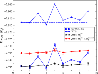
Figure 2: (Color online) AFQMC and LDA Si $\beta$-tin energies at nine randomly-chosen $\mathbf{k}$ points in the Brillouin zone of $3\times 3\times 3$ supercell. The AFQMC and LDA one-body FS errors are correlated, and the correction in Eq. (24) reduces the variation in the QMC data. The two-body FS error is significant even with a 54-atom supercell, but is essentially independent of $\mathbf{k}$-points.

The two-body FS error comes from the artificially induced periodicity of the long-range electron-electron Coulomb repulsion, due to the use of periodic boundary conditions. This error can be reduced significantly, using the post-processing correction scheme of Kwee et al.,Kwee et al. (2008b) which is based on a finite-size DFT xc functional, corresponding to the finite-sized supercell. This two-body correction is given by

$$\begin{split}\Delta E^{\textrm{Coulomb}}_{\mathbf{k}}=E^{\textrm{DFT},\infty}_{\mathbf{k}}-E^{\textrm{DFT},L}_{\mathbf{k}}\end{split}$$ (25)

where $E^{\textrm{DFT},\infty}_{\mathbf{k}}$ [$=E^{\textrm{DFT}}_{\mathbf{k}}$ in Eq. (24)] is the DFT energy computed with the usual LDA xc functional, while $E^{\textrm{DFT},L}_{\mathbf{k}}$ is the DFT energy computed with the finite-size LDA xc functional.Kwee et al. (2008b) The $\mathbf{k}$-dependence of $\Delta E^{\textrm{Coulomb}}_{\mathbf{k}}$ is very small compared to that of the one-body correction shown in Fig. 2, with variations of $\simeq 0.1\textrm{m}E_{\textrm{h}}$ in $\beta$-tin.

The total FS correction is the result of applying the one- and two-body correction terms, Eqs. (24) and (25), respectively. This is of course equivalent to applying $\Delta E_{\mathbf{k}}=E^{\textrm{DFT}}-E^{\textrm{DFT},L}_{\mathbf{k}}$ to the raw AFQMC energies. The corrected energies are averaged over the $\mathbf{k}$ points. The net effect of applying both FS corrections is to decrease the energy difference at the transition volumes from 34(1) to 29(1) $\textrm{m}E_{\textrm{h}}$. With these combined FS corrections, the residual errors in the absolute energies from $3\times 3\times 3$ supercells are expected to be small in silicon. Kwee et al. (2008b) Error cancellation in the energy difference between $\beta$-tin and diamond structures further reduces the error in the calculated transition pressure.

IV Results and Discussion

IV.1 Benchmarking the phaseless approximation with exact free-projection AFQMC

The fermionic sign/phase constraints used by QMC methods generally introduce uncontrolled approximations. Examples include the DMC fixed-node approximation and AFQMC phaseless constraint. Except where benchmarks with exact methods or experiment are available for comparison, the corresponding constraint errors are difficult to quantify. In this section, we show that exact free-projection calculations are feasible for the primitive diamond and $\beta$-tin structures, using planewave AFQMC on a large parallel computing platform. Comparison with the corresponding approximate phaseless AFQMC calculations shows that the systematic error due to the phaseless constraint is small (within 0.5 m$E_{\textrm{h}}$ /atom), as described below.

As illustrated in Fig. 3 for the diamond structure, free-projection to the ground state can be achieved in the primitive cell using large walker populations. The free-projection calculation was done with a target population size of two million walkers, using about 2000 cores at the NCCS Jaguar XT4 computer at Oak Ridge National Laboratory. An acceptable signal-to-noise ratio is sustained for sufficiently long imaginary times. For projection times $\beta>\sim 16E_{\textrm{h}}^{-1}$, however, growing fluctuations, due to the phase problem, begin to emerge. Eventually the fluctuations become severe enough to destroy the Monte Carlo signal.Zhang and Krakauer (2003) The energy measurement for this benchmark is taken after the walkers are sufficiently equilibrated, $\beta>10E_{\textrm{h}}^{-1}$. Similar calculations were performed in the $\beta$-tin structure.

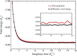
Figure 3: (Color online) Comparison of phaseless AFQMC with exact free-projection. The calculations shown are for the primitive cell in the diamond structure at the experimental equilibrium lattice constant ($10.264\,a_{0}$). The calculations used $L$ as the $\mathbf{k}$-point, and a time step size of $\tau=0.025E_{\textrm{h}}^{-1}$.

Figures 4 and 5 display extrapolations of the Trotter time step, $\tau$, for the diamond and $\beta$-tin structures, respectively. The figures compare the local-energy and hybrid phaseless methods with free-projection results. As $\tau\to 0$, the local-energy and hybrid phaseless methods are seen to converge to the same result, as expected, but with different slopes. To leading order, free-projection shows $\tau^{2}$ behavior, while the local-energy and hybrid methods have linear $\tau$ behavior, since the phaseless constraint (and the bounds in Sec. II.4) in the latter two methods break the quadratic scaling in Eq. (2). The hybrid method in Figs. 4 and 5 is seen to have the largest slope. The Trotter behaviors of the respective methods are similar in the diamond and $\beta$-tin structures.

The error in the total energy caused by the phaseless approximation, after extrapolation to $\tau\to 0$, is about $0.7\textrm{m}E_{\textrm{h}}$ (or $0.35\textrm{m}E_{\textrm{h}}$ per atom) for diamond and $0.8\textrm{m}E_{\textrm{h}}$ in $\beta$-tin. Note that the energy calculated from the phaseless approximation using the mixed-estimate [Eq. (14)] is not variational Zhang and Krakauer (2003). Indeed in both cases above it is below the exact result.

Table 2: AFQMC energies of Si diamond and $\beta$-tin phases for the 2-atom primitive cells, with volumes of $40.07$ Å³ and $30.00$ Å³, respectively. The $\beta$-tin $c/a$ ratio was set to 0.552. Phaseless AFQMC values are from the local energy formalism. Energies are in $E_{\textrm{h}}$ units.

phase	reduced $\mathbf{k}$ vector	free projection	phaseless
diamond	$(0.5,0.5,0.5)$	$-8.05485(8)$	$-8.0555(1)$
$\beta$-tin	$(0.25,0.25,0.25)$	$-8.1256(1)$	$-8.1264(1)$
$\beta$-tin	$(0.25,-0.25,0.25)$	$-8.0023(2)$	$-8.0017(2)$

In Table 2, we list the absolute energies for three cases from our free-projection calculations, which can serve as benchmarks in the future. All the energies have been extrapolated to $\tau\to 0$. The corresponding phaseless results are also listed, which are in very good agreement with the exact results. We note that the two twist boundary conditions ($\mathbf{k}$ points) in $\beta$-tin show different behaviors. In $\mathbf{k}=(0.25,0.25,0.25)$ the phaseless energy is below the exact value (as in the diamond case), while in the other, the phaseless energy is above. This manifests the varying quality of the trial wave function at the different $\mathbf{k}$-points, which shift the single-particle energy levels differently. Also, the FS effects are clearly very large in these small cells, where the energy for the first $\mathbf{k}$-point is in fact below that of the diamond result.

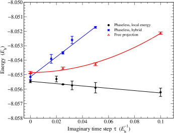
Figure 4: (Color online) Trotter time step $\tau$ extrapolation for the diamond structure, as in Fig. 3, comparing local-energy and hybrid phaseless methods with free-projection.

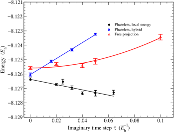
Figure 5: (Color online) Trotter time step $\tau$ extrapolation for the $\beta$-tin structure, comparing the local-energy phaseless method with free-projection. Calculations are for the primitive unit cell with volume of $30$ ų and $c/a=0.552$ at the reduced $\mathbf{k}$ = (0.25, 0.25, 0.25).

IV.2 Transition pressure

AFQMC calculations were done for $3\times 3\times 3$ supercells (containing 54 silicon atoms), at the experimental transition volumes, McMahon et al. (1994) $36.30$ Å³ for the diamond and $27.91$ Å³ for the $\beta$-tin structures. For $\beta$-tin, we used the experimental value of $c/a=0.550$. Hu et al. (1986) (It was shown in LABEL:Alfe2004 that the dependence on $c/a$ is weak.) Twist averaged boundary conditions used the single special $\mathbf{k}$-point of Baldereschi Baldereschi (1973) for the diamond structure, and nine random $\mathbf{k}$ points for the $\beta$-tin phase. The total energies lead to a “raw” transition pressure of $15.1(3)$ GPa.

To compare with experiment, corrections are required to account for zero-point motion and thermal effects. We apply these corrections as given in LABEL:Alfe2004: 1) a zero-point motion lowering of 0.3 GPa; 2) a room-temperature quasi-harmonic estimate of the relative stabilization of the $\beta$-tin phase, which lowers the pressure by 1.15 GPa. This would give a transition pressure of $13.6(3)$ GPa. In addition, standard mean-field pseudopotentials generated from LDA or HF, such as the one used in the present paper, do not account for many-body effects in the core. A correction was estimated in LABEL:Alfe2004, by explicitly including a many-body core polarization potential (CPP), which further lowers the pressure by $\sim 1.2$ GPa. Assuming that our LDA pseudopotential is similar to that in LABEL:Alfe2004, we apply the same correction. Table 3 reports our final result, and compares it to experiment and to other theoretical results. Corrections (1) and (2) have also been applied to the DFT results.

Table 3: The transition pressure $P_{t}$ of the diamond to $\beta$-tin transition in silicon. The AFQMC result is listed together with experimental and other theoretical results. To compare with experiment, appropriate corrections have been applied to the theoretical results (see text).

Method	$P_{t}$ (GPa)
LDANeeds and Mujica (1995)	6.7
GGA (BP)Moll et al. (1995)	13.3
GGA (PW91)Moll et al. (1995)	10.9
DMCAlfè et al. (2004)	16.5(5)
AFQMC	12.6(3)
ExperimentMujica et al. (2003)	10.3–12.5

The transition pressure is not very sensitive to the choice of transition volumes. For example, using the DMC predicted volumes instead of the experimental values changes the energy difference by only $0.01$ eV, from $0.49$ to $0.50$ eV, reducing the transition pressure by less than $0.3$ GPa.

The best calculation to date with the highest level of theory is the DMC calculations in LABEL:Alfe2004. Compared to experiment, the somewhat overestimated DMC $P_{t}=16.5(5)$ value was attributed to the fixed-node error.Alfè et al. (2004) This seems consistent with our results. The DMC discrepancy corresponds to a larger “raw” energy difference of $19.2\,\textrm{m}E_{\textrm{h}}$ between the two phases, compared to $15.1(3)\,\textrm{m}E_{\textrm{h}}$ for phaseless AFQMC. As shown in the previous subsection, the error due to the phaseless approximation ($\simeq 0.5\,\textrm{m}E_{\textrm{h}}$) appears to be an order of magnitude smaller than this. Our calculations show that experiment and theory are in quantitative agreement on the diamond to $\beta$-tin transition.

V Summary

We have applid the phaseless auxiliary-field quantum Monte Carlo method to study the pressure-induced structural phase transition from diamond to $\beta$-tin in silicon. This is a recently developed non-perturbative, many-body approach which recovers electron correlation by explicitly summing over fluctuating mean-field solutions with Monte Carlo. The only source of error which can not be systematically driven to zero is that of the global phase constraint, used to control the sign/phase problem. We quantified the systematic error from this phaseless approximation by exact unconstrained AFQMC calculations in the primitive cell, carried out on large parallel computers. In both structural phases the error was found to be well within 0.5m$E_{\textrm{h}}$/atom. A transition pressure was calculated form the energy difference between the two phases at the experimental transition pressure, using 54-atom supercells. Twist-averaging boundary condition and finite-size corrections were applied, which greatly accelerates the convergence to the thermodynamic limit. After corrections for zero-point effect, thermal effect, and the (lack of) core-polarization in the pseudopotential, the AFQMC results yield a transition pressure of $12.6\pm 0.3$ GPa, compared to experimental values of $10.3$-$12.5$ GPa.

The good agreement between the phaseless AFQMC result and experiment is consistent with the internal benchmark with unconstrained AFQMC. Our analysis indicates that the possible combined error from the calculations should be below $1$ GPa. These include pseudopotential transferability errors and core-polarization effect, residual finite-size errors, and the error from the phaseless approximation.