A consistent statistical treatment of the renormalized mean - field t-J model

Abstract

A variational treatment of the Gutzwiller - renormalized t-J Hamiltonian combined with the mean-field (MF) approximation is proposed, with a simultaneous inclusion of additional consistency conditions. Those conditions guarantee that the averages calculated variationally coincide with those calculated from the self-consistent equations. This is not ensured a priori because the effective Hamiltonian contains renormalization factors which depend explicitly on the mean-field averages. A comparison with previous mean-field treatments is made for both superconducting (d-RVB) and normal states and encompasses calculations of both the superconducting gap and the renormalized hopping amplitudes, as well as the electronic structure. The $C_{4v}$-symmetry breaking in the normal phase - the Pomeranchuk instability (PI) - is also analyzed.

t-J model Spalek Oles is regarded to reflect some of the essential physics of strongly correlated copper $3d_{x^{2}-y^{2}}$ states in high-temperature superconductors.Lee In this model, the correlated hopping of electrons reduces strongly their band energy, so the latter, for the doping $x\leq 0.1$, becomes comparable to the real-space pairing part induced by the kinetic exchange.Spalek didactical tJ However, the analytical solutions of t-J model are limited to the special cases for the one-dimensional system.Sarben Sarkar Under these circumstances, we have to resort to either exact diagonalization,Freericks Falicov which is limited to small cluster systems or to the approximate methods. The latter include renormalization group,Falicov Berker variational approach based on the Gutzwiller - projected wavefunctions (either treated within Monte Carlo techniques or by Gutzwiller approximationEdegger ) and various versions of the slave - boson approach.Lee Each of these methods seizes some of the principal features of these quasi-two-dimensional correlated states, although no coherent picture has emerged as yet.

In this paper we concentrate on the Gutzwiller renormalized mean-field (MF) theory for the t-J Hamiltonian and formulate a variational procedure, with the additional conditions ensuring the self-consistency of the whole approach. Implementing such procedure is essential (if not indispensable) for obtaining reliable results of the MF type. It is reassuring that some of the quantities such as the RVB gap magnitude or the hopping correlations (bond-parameter) do not change appreciably with respect to the earlier results,Marcin Polonica whereas the others, such as the single-particle electronic structure, are altered remarkably. Furthermore, we illustrate the basic nontriviality of our approach on the example of the so-called Pomeranchuk instability discussed recently.H. Yamase and H. Kohno

We start with the t-J model in its simplest form,Spalek Oles ; Lee

$$\hat{H}_{tJ}=\hat{P}\big{(}\sum_{i,j,\sigma}t_{ij}c_{i\sigma}^{{\dagger}}c_{j\sigma}+\sum_{\langle ij\rangle}J_{ij}~{}\mathbf{S}_{i}\cdot\mathbf{S}_{j}-\mu\sum_{i,\sigma}\hat{n}_{i\sigma}\big{)}\hat{P},$$ (1)

where $\hat{P}$ labels the Gutzwiller projector which guarantees that no doubly occupied sites are present. The projected operators and the model parameters have the standard meaning.Spalek Oles

To proceed further, effective mean-field renormalized Hamiltonian is introduced Edegger ; Marcin Polonica ; ZGRS ; The ladder of Sigrist ; Didier ; Marcin 1 ; LiZhouWang ; Ogata Himeda which is taken in the following form

$$\hat{H} = \sum_{\langle ij\rangle\sigma}\big{(}t_{ij}g^{t}_{ij}c_{i\sigma}^{{\dagger}}c_{j\sigma}+\text{H.c.}\big{)}-\mu\sum_{i\sigma}c^{{\dagger}}_{i\sigma}c_{i\sigma}$$ (2)

$$- \sum_{\langle ij\rangle\sigma}\frac{3}{4}J_{ij}g^{J}_{ij}(\chi_{ji}c_{i\sigma}^{{\dagger}}c_{j\sigma}+\text{H.c.}-|\chi_{ij}|^{2})$$

$$- \sum_{\langle ij\rangle\sigma}\frac{3}{4}J_{ij}g^{J}_{ij}(\Delta_{ij}c^{{\dagger}}_{j\sigma}c_{i-\sigma}^{{\dagger}}+\text{H.c.}-|\Delta_{ij}|^{2}).$$

In the above expression, $c_{i\sigma}^{{\dagger}}$ ($c_{j\sigma}$) are ordinary fermion creation (annihilation) operators, $\chi_{ij}=\langle c_{i\sigma}^{{\dagger}}c_{j\sigma}\rangle$, and $\Delta_{ij}=\langle c_{i-\sigma}c_{j\sigma}\rangle=\langle c_{j-\sigma}c_{i\sigma}\rangle$ are respectively, the hopping amplitude (bond-parameter) and the RVB gap parameter, both taken for nearest neighbors $\langle ij\rangle$. The renormalization factors $g^{t}_{ij}$ and $g^{J}_{ij}$ result from the Gutzwiller ansatz. The exchange part ($\mathbf{S}_{i}\cdot\mathbf{S}_{j}$) has been decoupled in the Hartree-Fock-type approximation and incorporates as nonzero all above bilinear averages obtained according to the prescription

$$\hat{O}_{\kappa}\hat{O}_{\gamma}\to\hat{A}_{s}A_{t}+A_{s}\hat{A}_{t}-A_{s}A_{t},$$ (3)

where $t=t(\kappa,\gamma)$ etc. and for any operator $\hat{A}$

$$A=\langle\hat{A}\rangle\equiv\text{Tr}[\hat{A}\hat{\rho}],$$ (4)

with $\hat{\rho}$ being the density matrix for the mean-field Hamiltonian to be determined. By taking the step from (1) to (2) we introduce essentially a non-Hartree-Fock-type of approximation, which differs from (3) due to the presence of $g^{t}_{ij}$ and $g^{J}_{ij}$ factors. Therefore, we may not be able use e.g. the density operator of the form $\hat{\rho}=Z^{-1}e^{-\beta\hat{H}}$, $Z=\text{Tr}[e^{-\beta\hat{H}}]$, as a proper grand-canonical trial state in the frame of variational principle based on the Bogoliubov inequality,Feynman since then the self-consistency of the approach (expressed by Eq.(4)) may be violated. This is the reason, why in most of the previous mean field treatments, e.g. Marcin Polonica ; The ladder of Sigrist ; Didier ; Marcin 1 , the standard procedure encompasses diagonalizing of the bilinear Hamiltonian (2), and subsequently solving of the self-consistent (s-c) Bogoliubov-de Gennes (BdG) equations for $\chi_{ij}$, $\Delta_{ij}$ and $\mu$. In effect, this procedure does not refer to any variational scheme.

The solution based solely on the s-c BdG equations, although acceptable, may not be fully satisfactory. This is because in the present situation we build up the entire description on the basis of MF Hamiltonian and hence we should proceed in a direct analogy to the exact (non-MF) case. Namely, our approach is based on the maximum entropy principle.Jaynes Such starting point provides us with a general variational principle, which may differ from that of Bogoliubov and Feynman.Feynman In other words, the value of the appropriate functional is minimized, with the self-consistency of the whole approach being preserved at the same time.JJJS_arx_0

To tackle the situation, we define an effective Hamiltonian $\hat{H}_{\lambda}$ containing additional constraints, that is of the form

$$\hat{H}_{\lambda}=\hat{H} - \sum_{i}\lambda^{(n)}_{i}\big{(}\sum_{\sigma}c_{i\sigma}^{{\dagger}}c_{i\sigma}-n_{i}\big{)}$$ (5)

$$- \sum_{\langle ij\rangle\sigma}\big{(}\lambda^{\chi}_{ij}(c_{i\sigma}^{{\dagger}}c_{j\sigma}-\chi_{ij})+\text{H.c.}\big{)}$$

$$- \sum_{\langle ij\rangle\sigma}\big{(}\lambda^{\Delta}_{ij}(c_{i-\sigma}c_{j\sigma}-\Delta_{ij})+\text{H.c.}\big{)},$$

where the Lagrange multipliers $\lambda^{(n)}_{i}$, $\lambda^{\chi}_{ij}$, and $\lambda^{\Delta}_{ij}$ play the role of molecular fields. Moreover, the parameters $\chi_{ij}$, $\Delta_{ij}$, and $n_{i}=\sum_{\sigma}\langle c_{i\sigma}^{{\dagger}}c_{i\sigma}\rangle$ coincide with those which appear in the renormalization factors $g^{t}_{ij}$ and $g^{J}_{ij}$, and which are taken in the form Marcin Polonica ; Marcin 1

$$g^{t}_{ij}=\sqrt{\frac{4x_{i}x_{j}(1-x_{i})(1-x_{j})}{(1-x_{i}^{2})(1-x_{j}^{2})+8(1-x_{i}x_{j})|\chi_{ij}|^{2}+16|\chi_{ij}|^{4}}},$$

$$g^{J}_{ij}=\frac{4(1-x_{i})(1-x_{j})}{(1-x_{i}^{2})(1-x_{j}^{2})+8x_{i}x_{j}\beta^{-}_{ij}(2)+16\beta^{+}_{ij}(4)},$$ (6)

with $x_{i}\equiv 1-n_{i}$, $\beta^{\pm}_{ij}(n)=|\Delta_{ij}|^{n}\pm|\chi_{ij}|^{n}$.

When solving the model on a square lattice and in the spatially homogeneous case, there appear thus five mean fields, $\vec{A}\equiv(n,\chi_{x},\chi_{y},\Delta_{x},\Delta_{y})$, with $\chi_{\tau}=\chi_{ij},\Delta_{\tau}=\sqrt{2}\Delta_{ij}$, ($\langle ij\rangle||\tau$, $\tau=x,y$; as well as the same number of the corresponding Lagrange multipliers, $\vec{\lambda}\equiv(\lambda,\lambda^{\chi}_{x},\lambda^{\chi}_{y},\lambda^{\Delta}_{x},\lambda^{\Delta}_{y})$, where $\lambda^{\chi}_{\tau}=\lambda^{\chi}_{ij},\lambda^{\Delta}_{\tau}=\sqrt{2}\lambda^{\Delta}_{ij}$. Both $\vec{A}$ and $\vec{\lambda}$ are assumed to be real. Apart from that, for given $n$ we have to determine the chemical potential $\mu$. The first step is the diagonalization of $\hat{H}_{\lambda}$ via Bogoliubov-Valatin transformation, which yields

$$\hat{H}_{\lambda}=\sum_{\mathbf{k}}E_{\mathbf{k}}(\hat{\gamma}^{{\dagger}}_{\mathbf{k}0}\hat{\gamma}_{\mathbf{k}0}+\hat{\gamma}^{{\dagger}}_{\mathbf{k}1}\hat{\gamma}_{\mathbf{k}1})+\sum_{\mathbf{k}}(\xi_{\mathbf{k}}-E_{\mathbf{k}})+C,$$ (7)

with $E_{\mathbf{k}}=\sqrt{\xi^{2}_{\mathbf{k}}+D^{2}_{\mathbf{k}}}$, $D_{\mathbf{k}}=\sqrt{2}\sum_{\tau}D_{\tau}\cos(k_{\tau})$, and $\xi_{\mathbf{k}}=-2\sum_{\tau}T_{\tau}\cos(k_{\tau})-\mu-\lambda$. Also,

$$T_{\tau}=-t_{1\tau}g^{t}_{1\tau}+\frac{3}{4}J_{\tau}g^{J}_{\tau}\chi_{\tau}+\lambda^{\chi}_{\tau},~{}~{}~{}~{}D_{\tau}=\frac{3}{4}J_{\tau}g^{J}_{\tau}\Delta_{\tau}+\lambda^{\Delta}_{\tau},$$ (8)

$$\frac{C}{\Lambda}=\lambda n+\sum_{\tau}\big{(}\frac{3}{4}J_{\tau}g^{J}_{\tau}(2\chi^{2}_{\tau}+\Delta^{2}_{\tau})+4\chi_{\tau}\lambda^{\chi}_{\tau}+2\Delta_{\tau}\lambda^{\Delta}_{\tau}\big{)}.$$ (9)

For the sake of simplicity, we have included only the hopping between the nearest neighbors, although the generalization to the case with more distant hopping does not pose any principal difficulty. We define next the generalized Landau functional, $\mathcal{F}\equiv-\beta^{-1}\ln(\text{Tr}[e^{-\beta\hat{H}_{\lambda}}])$, which here takes the form

$$\mathcal{F}(\vec{A},\vec{\lambda})=C+\sum_{\mathbf{k}}\big{(}(\xi_{\mathbf{k}}-E_{\mathbf{k}})-\frac{2}{\beta}\ln\big{(}1+e^{-\beta E_{\mathbf{k}}}\big{)}\big{)},$$ (10)

with inverse temperature $\beta=1/k_{B}T$. The equilibrium values of $\vec{A}=\vec{A}_{0}$, $\vec{\lambda}=\vec{\lambda}_{0}$ are the solution of the set of equations

$$\nabla_{A}\mathcal{F}=0,~{}~{}~{}~{}\nabla_{\lambda}\mathcal{F}=0,$$ (11)

for which (10) reaches its minimum. This step is equivalent to the maximization of the entropy with the constraints.JJJS_arx_0 Also, the grand potential $\Omega$ and the free energy $F$ are defined respectively as $\Omega(T,V,\mu)=\mathcal{F}(T,V,\mu;\vec{A}_{0}(T,V,\mu),\vec{\lambda}_{0}(T,V,\mu))$, and $F=\Omega+\mu N$. Note, that by taking the derivatives with respect to $\vec{\lambda}$ only, and subsequently putting $\vec{\lambda}=\vec{0}$, the results reduce to the standard BdG self-consistent equations.

Even though the present method can be regarded as natural within the context of statistical mechanics, to the best of our knowledge, it has not been utilized, in the form presented here, in the context of condensed matter physics problems. Also, in this respect, our approach unifies individual features of the self-consistent variational MF treatments developed earlierBuenemann Gebhard Thul ; Ogata Himeda ; LiZhouWang ; Wang F C Zhang , which in the $T=0$ limit can be obtained as particular cases. Parenthetically, the present method, together with the Gutzwiller approximation, provides also a natural justification of some aspects of the slave-boson saddle-point approach, as some of the constraints coincide in both methods.

We solve numerically first the system of equations (11) on the lattice of $\Lambda=128\times 128$ sites, using the periodic boundary conditions and taking the parameters $J_{x}=J_{y}=J=1$, $t_{x}=t_{y}=-3J$, and for low temperature $k_{B}T/J=0.002$ for the filling $n=7/8=0.875$. Both the d-wave superconducting resonating valence bond (d-RVB) and the isotropic normal (N) solutions are analyzed. The self-consistent variational results (denoted as var) obtained here and those obtained from BdG equations are compared in Tables I and II. One sees that our value of the low-temperature free energy (per site), (c.f. Table I) in the d-RVB phase is slightly better than the previous estimates,Marcin Polonica ; Marcin 1 albeit not much ($-1.3661$ for var, as compared to $-1.3647$ for s-c). It is slightly higher than that of the Variational Monte Carlo, which is $E_{VMC}/J=-1.3671$, c.f.Marcin 1 Also the isotropic staggered-flux (SF) phase has been found unstable against N state within both methods at this filling. In Table II we display microscopic quantities characterizing each solution in that case and compare them with those obtained within standard s-c treatment. The differences are more pronounced for the RVB state.

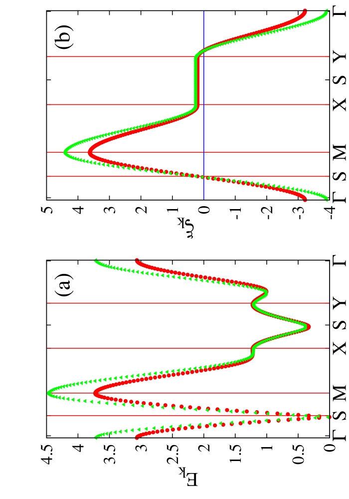
Figure 1: (Color online) Dispersion relations along the main symmetry lines in the Brillouin zone for a square lattice, of the size $\Lambda_{x}=\Lambda_{y}=128$, and for the filling $n=0.875$. Left (a): d-RVB solutions, right (b): N solutions. Triangles - earlier self-consistent results, circles - the present method.

For the parameters listed in Tables I and II we have computed the quasiparticle energies in both the d-RVB and the N states. Those are shown in Fig. 1a-b. The solid circles represent our results, whereas the previous ones Marcin Polonica are drawn as triangles. The energy-dispersion reduction in our case is connected with presence of the constraints and results in a decrease of the bandwidth, which, in turn, is regarded as a sign of enhanced electron correlations.

After testing the feasibility of our approach for fixed doping $x$, we now discuss systematic changes appearing as the function of $x$, as shown in Figs. 2 and 3.

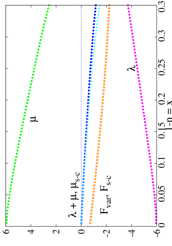
Figure 2: (Color online) Doping dependences of the free energy ($F_{var},F_{s-c}$), the chemical potentials $\mu$, $\mu_{s-c}$ as well as that of $\lambda$ and $\lambda+\mu$ for the d-RVB state, both within the present (var) and the standard (s-c) methods.

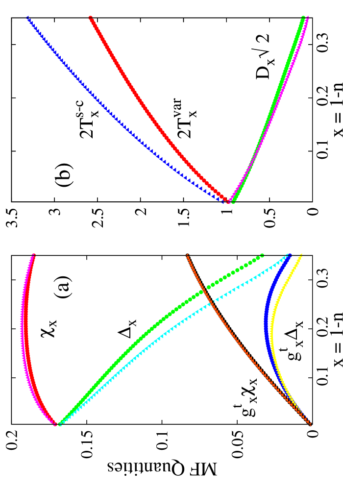
Figure 3: (Color online) Left: Doping dependence of the bond-order parameters $\chi_{x}=\chi_{y}$, the superconducting order parameters $\Delta_{x}=-\Delta_{y}$, their renormalized counterparts $g^{t}\chi_{x}=g^{t}\chi_{y}$ and $g^{t}\Delta_{x}=-g^{t}\Delta_{y}$, as well as (right) of the quantities $2T_{x}=2T_{y}$ and $\sqrt{2}D_{x}=-\sqrt{2}D_{y}$ of Eq. (8), both for the s-c (triangles) and the var (circles) methods.

We emphasize, the chemical potential $\mu$ is the first derivative of $F/\Lambda$ with respect to $n$ (c.f. Fig.2), unlike in some of the previous mean-fields treatments Marcin Polonica ; The ladder of Sigrist ; Didier ; Marcin 1 (c.f. however Ref. ZGRS ; Buenemann Gebhard Thul ). This is also the reason why we differentiate between $\mu$ and $\tilde{\mu}\equiv\mu+\lambda$, even in the case of the spatially homogeneous solution. The doping dependence of other relevant MF quantities is shown in Fig.3. The results are again close to those obtained from the BdG procedure, except for $T_{\tau}$, (Fig.3(b)), which enter the quasiparticle energies.

So far we have focused on MF solutions with the symmetry between $x$ and $y$ directions on the square lattice.Ladder of J However, a spontaneous breakdown of this equivalence of the $x$- and $y$- directed correlations is possible already in the normal phase and is called the Pomeranchuk instability (PI), H. Yamase and H. Kohno that manifests itself by lowering of the discrete $C_{4v}$ symmetry of the Fermi surface.

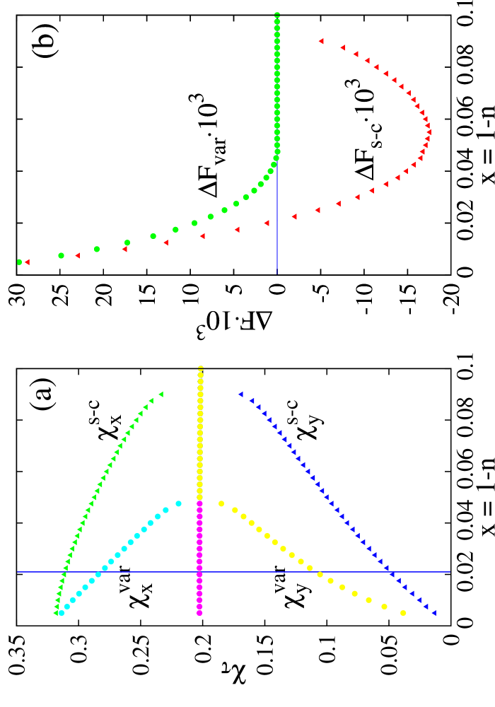
Figure 4: (Color online) Doping dependence of bond-order parameters $\chi_{x}$ and $\chi_{y}$ (left), and the free-energy differences $\Delta F$ (right) both for $x$-$y$ symmetric (N) and the Pomeranchuk (x-y symmetry-broken) states (PI) within both the present(var, filled circles) and the standard (s-c, triangles) methods, respectively. The vertical line marks the phase transition within the s-c method. For details, see main text.

In Fig. 4 (a) the doping dependence of the bond-order parameters $\chi_{x}$ and $\chi_{y}$ are displayed for the $x$-$y$ symmetric (N) and the symmetry-broken (PI) solutions, both within our ($\chi^{var}_{\tau}$) and the standard ($\chi^{s-c}_{\tau}$) methods. Within the s-c scheme, PI solution is found up to $x\approx 0.091$. However, a comparison of the respective free-energy differences, $\Delta F_{s-c}\equiv F_{s-c}^{N}-F_{s-c}^{PI}$ and $\Delta F_{var}\equiv F_{var}^{N}-F_{var}^{PI}$, (cf. Fig. 4 (a)) reveals that this solution becomes unstable against N state for $x\approx 0.021$, thus the phase transition is certainly discontinuous. On the other hand, within our variational treatment the PI solution does not exist for $x>x^{var}_{c}\approx 0.044$, where $\Delta F_{var}\approx 0$, in qualitative agreement with what is expected for the continuous phase transition.From this analysis it is clear that the two methods of approach (s-c, var) yield qualitatively different predictions for PI.

In summary, we have introduced self-consistency constraints required within the variational mean-field approach to the Gutzwiller-renormalized mean-field t-J model. Such consistency conditions are indispensable from the basic statistical-mechanical point of view. Undertaking such a step results in consistent evaluations of the thermodynamic quantities, which in the present method are determined from the generalized Landau functional. A detailed comparison with the standard mean-field solution based on Bogoliubov-de Gennes self-consistent equations (i.e. that without constraints) is provided. Our method introduces quantitative and, in some cases, even qualitative corrections to the standard mean-field results. Other mean-field states such as flux phases or antiferromagnetism can be treated in the same manner.

The authors are very grateful to Marcin Raczkowski and Andrzej Kapanowski for valuable comments and technical help. All the numerical computations were performed using GSL (Gnu Scientific Library) efficient procedures. The work was supported by the Grant No. N N 202 128 736 from the Ministry of Science and Higher Education, as well as by the National Network Strongly Correlated Electrons and the European COST Network (ECOM).

References

- (1) For the original derivation from Hubbard model see K. A. Chao, J. Spałek, A. M. Oleś, J. Phys. C 10, L271 (1977). For its physical applicability to high-temperature superconductors see: P. W. Anderson, in: Frontiers and Borderlines in Many-Particle Physics, edited by R.A. Broglia and J. R. Schriefer (North-Holland, Amsterdam, 1988) p.1 ff; F. C. Zhang and T. M. Rice, Phys. Rev. B 37, 3759 (1988); A. E. Ruckenstein, P. J. Hirschfeld, and J. Appel, Phys. Rev. B 36, 857 (1987); For exact projections of pairing operators see: J. Spałek, Phys. Rev. B 37, 533 (1988); N. M. Plakida, R. Hayn, and J.-L. Richard, Phys. Rev. B 51, 16599 (1995).
- (2) For review, see: P. A. Lee in Handbook of High-Temperature Superconductivity, edited by J. R. Schriefer and J. S. Brooks (Springer Science, New York, 2007) chapter 14; M. Ogata and H. Fukuyama, Rep. Prog. Phys. 71, 036501 (2008); P. A. Lee, N. Nagaosa and X-G Wen, Rev. Mod. Phys 78, 17 (2006) and References therein.
- (3) For didactical discussion, see e.g. J. Spałek, Acta Phys. Polon. A 111, 409 (2007).
- (4) S. Sarkar, Physica B 206-207, 723 (1995), see also: F. H. L. Essler, H. Frahm, F. Görmann, A. Klümper, and V. E. Korepin, The One-Dimensional Hubbard Model. Cambridge University Press, 2005.
- (5) J. K. Freericks and L. M. Falicov, Phys. Rev. B 42, 4960 (1990).
- (6) A. Falicov and A. N. Berker Phys. Rev. B 51, 12458 (1995).
- (7) B. Edegger, V. N. Muthukumar, and C. Gros, Adv. Phys. 56, 927 (2007).
- (8) M. Raczkowski, Acta Phys. Polon. A 114, 107 (2008).
- (9) H. Yamase and H. Kohno, J. Phys. Soc. Jpn. 69, 332, (2000); ibid. 69, 2151, (2000); L. Dell’Anna and W. Metzner, Phys. Rev. B 73, 045127 (2006); A. Miyanaga and H. Yamase , Phys. Rev. B 73, 174513, (2006); B. Edegger, V. N. Muthukumar, and C. Gros, Phys. Rev. B 74, 165109, (2006); H. Yamase and W. Metzner, Phys. Rev. B 75, 155117 (2007); H. Yamase, arXiv:0907.4253 (2009).
- (10) F. C. Zhang, C. Gros, T. M. Rice, and H. Shiba, Supercond. Sci. Technol. 1 36, (1988).
- (11) M. Sigrist, T. M. Rice, and F.C. Zhang, Phys. Rev. B 49, 12 058 (1994).
- (12) D. Poilblanc, Phys. Rev. B 72, 060508(R) (2005).
- (13) M. Raczkowski, M. Capello, D. Poilblanc, R. Frésard, and A. M. Oleś, Phys. Rev. B 76, 140505(R) (2007); M. Raczkowski, M. Capello and D. Poilblanc, Acta Phys. Polon. A 115, 77 (2009).
- (14) J. Bünemann, F. Gebhard and R. Thul, Phys. Rev. B 67, 075103 (2003).
- (15) M. Ogata, A. Himeda, J. Phys. Soc. Jpn. 72, 374, (2003).
- (16) C. Li, S. Zhou and Z. Wang, Phys. Rev. B 73, 060501(R), (2006).
- (17) Qiang-Hua Wang, Z. D. Wang, Yan Chen, and F. C. Zhang, Rev. B 73 092507 (2006).
- (18) R. P. Feynman, Statistical Mechanics, (W. A. Benjamin 1972), chapter 2.
- (19) E. T. Jaynes, Phys. Rev. 106, 620-630 (1957); ibid. 108, 171-190 (1957).
- (20) J. Jȩdrak and J. Spałek, arXiv:0804.1376 (unpublished).
- (21) The modifications introduced in our approach are relevant also for a two-leg ladder systems,The ladder of Sigrist but the results are not discussed here.