NN potentials from IR chiral EFT

Abstract:

Chiral perturbation theory is nowadays a well-established approach to incorporate the chiral constraints from QCD. Nevertheless, for systems involving one baryon, the power counting which dictates the chiral order of observables is not as simple and consensual as in the purely mesonic case. The heavy baryon approach, which relies on a non-relativistic expansion around the limit of infinitely heavy baryon, recovers the usual power counting but destroys some analytic properties of the scattering amplitude. Some years ago, Becher and Leutwyler proposed a Lorentz-invariant formulation of chiral perturbation theory that maintains the required analytic properties, but at the expense of a less intuitive power counting.

Aware of the shortcomings of the heavy baryon formalism, the São Paulo group derived the two-pion exchange component of the nucleon-nucleon potential in line with the works of Becher and Leutwyler. A striking result was that the long distance properties of the potential is determined by the specific low energy region of the pion-nucleon scattering amplitude where the heavy baryon expansion fails. In this talk I will discuss the origin of such failure and how it reflects in the asymptotics of the nucleon-nucleon interaction. Some results for phase shifts and deuteron properties will be shown, followed by a comparison with the heavy baryon predictions.

1 Analyticity constraints

Becher and Leutwyler [1] demonstrated that, in the baryon sector, convergence of the chiral expansion of certain quantities (form factors, for instance) is a delicate issue. This is closely related to the presence of an anomalous threshold in the triangle diagram (l.h.s. of Fig.1) for momentum transfer $t$ close to the two-pion threshold, $4m_{\pi}^{2}$. Such analytic structure is completely missed in the usual heavy baryon (HB) formulation of chiral perturbation theory ($\chi$PT). It can only be recovered via a resummation of the HB series to all orders. To understand this issue (for more details, see for instance Ref. [2]) one starts with the spectral representation of the triangle integral,

$$\gamma(t)=\frac{1}{\pi}\int_{4m_{\pi}^{2}}^{\infty}\frac{dt^{\prime}}{(t^{\prime}\!-\!t)}\,\mbox{Im}\gamma(t^{\prime})\,,\quad\mbox{Im}\gamma(t^{\prime})\simeq\mbox{Im}\gamma(t^{\prime})|_{\rm BL}=\frac{\theta(t^{\prime}\!-\!4m_{\pi}^{2})}{16\pi m_{N}\sqrt{t^{\prime}}}\,\arctan\frac{2m_{N}\sqrt{t^{\prime}\!-\!4m_{\pi}^{2}}}{t^{\prime}\!-\!2m_{\pi}^{2}}\,.$$ (1)

The argument $x=2m_{N}\sqrt{t^{\prime}-4m_{\pi}^{2}}/(t^{\prime}-2m_{\pi}^{2})$ is formally counted as order $q^{-1}$ in the HB expansion, which yields $\tan^{-1}x=\pi/2-1/x+1/3x^{3}+\cdots$. In fact, the first two terms reproduce the HB result for the triangle graph,

$$\gamma(-q^{2})|_{\rm HB} = \frac{1}{16\pi^{2}m_{N}m_{\pi}}\int_{4m_{\pi}^{2}}^{\infty}\frac{dt^{\prime}}{(t^{\prime}+q^{2})}\,\frac{1}{\sqrt{t^{\prime}}}\left[\frac{\pi}{2}-\frac{(t^{\prime}-2m_{\pi}^{2})}{2m_{N}\sqrt{t^{\prime}\!-\!4m_{\pi}^{2}}}\right]$$ (2)

$$= \frac{1}{16\pi^{2}m_{N}m_{\pi}}\left[2\pi m_{\pi}\,A(q)+\frac{m_{\pi}}{m_{N}}\,\frac{(2m_{\pi}^{2}+q^{2})}{(4m_{\pi}^{2}+q^{2})}\,L(q)\right]\,,$$

where $q=|{\mbox{\boldmath$q$}}|$, and $L(q)$ and $A(q)$ are the usual HB loop functions,

$$L(q)=\frac{\sqrt{4m_{\pi}^{2}+q^{2}}}{q}\,\ln\frac{\sqrt{4m_{\pi}^{2}+q^{2}}+q}{2m_{\pi}}\,,\qquad\qquad A(q)=\frac{1}{2q}\,\arctan\frac{q}{2m_{\pi}}\,.$$ (3)

However, it does not take into consideration the case $|x|<1$, where $t^{\prime}$ gets closer to $4m_{\pi}^{2}$. This region controls the long distance behavior of the triangle diagram, as can be seen by its representation in configuration space [3, 4, 5],

$$\Gamma(r)=\frac{1}{\pi}\int_{4m_{\pi}^{2}}^{\infty}dt^{\prime}\int\frac{d^{3}q}{(2\pi)^{3}}\;e^{-i{\mbox{\boldmath$q$}}\cdot{\mbox{\boldmath$r$}}}\;\frac{\mbox{Im}\gamma(t^{\prime})}{t^{\prime}+q^{2}}=\frac{1}{4\pi^{2}}\int_{4m_{\pi}^{2}}^{\infty}dt^{\prime}\;\frac{e^{-r\sqrt{t^{\prime}}}}{r}\;\,\mbox{Im}\gamma(t^{\prime})\,.$$ (4)

Clearly one sees that, in order to have a good asymptotic description of $\Gamma(r)$, one needs a decent representation for $\mbox{Im}\gamma(t^{\prime})$ near $t^{\prime}=4m_{\pi}^{2}$, which cannot be provided by the usual HB formulation.

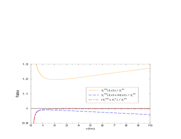
Figure 1: The triangle diagram that contributes to the nucleon scalar form factor. On the right panel are shown ratios of the two first terms of $\gamma(-q^{2})|_{\rm HB}$, divided by $\gamma(-q^{2})|_{\rm BL}$. For more details, see Ref. [3].

We want to stress that the expansion in $1/m_{N}$ of our two-pion exchange nucleon-nucleon potential (TPEP) should, in principle, recover the expressions from HB$\chi$PT. This can be used as a cross-check of our calculation (see next section). However one must keep in mind that, due to the problem described above, such an expansion is ill-defined at long distances and should be avoided.

2 The Lorentz-invariant two-pion exchange amplitude

The two-pion exchange (TPE) amplitude that contributes to the NN interaction is closely linked to the $\pi$N amplitude, which is generically expressed in terms of two invariant amplitudes $D^{\pm}(\nu,t)$ and $B^{\pm}(\nu,t)$,

$$T_{\pi{\rm N}}^{ab} = \delta_{ab}\,T_{\pi{\rm N}}^{+}+i\epsilon_{bac}\,\tau_{c}\,T_{\pi{\rm N}}^{-}\,,$$

$$T_{\pi{\rm N}}^{\pm} = \bar{u}({\mbox{\boldmath$p^{\prime}$}})\,\Big{[}D^{\pm}-\frac{i}{2m_{N}}\,\sigma_{\mu\nu}(p^{\prime}-p)^{\mu}\,\frac{(k+k^{\prime})^{\nu}}{2}\,B^{\pm}\Big{]}\,u({\mbox{\boldmath$p^{\prime}$}})\,,$$ (5)

where $p$ and $p^{\prime}$ are the initial and final momenta of the nucleon, respectively, while $\nu=[(p+k)^{2}-(p-k^{\prime})^{2}]/4m_{N}$ and $t=(k^{\prime}-k)^{2}$ are the usual Mandelstam variables. This allows the TPE amplitude to be written as

$${\cal T}_{\rm TPE}=-\frac{i}{2!}\int[\cdots]\left[3\,T_{\pi{\rm N}}^{(1)+}\,T_{\pi{\rm N}}^{(2)+}+2\,{\mbox{\boldmath$\tau$}}^{(1)}\cdot{\mbox{\boldmath$\tau$}}^{(2)}\,T_{\pi{\rm N}}^{(1)-}\,T_{\pi{\rm N}}^{(2)-}\right]$$ (6)

$$=\left[\bar{u}u\right]^{(1)}\left[\bar{u}u\right]^{(2)}{\cal I}_{DD}^{\pm}-\left[\bar{u}u\right]^{(1)}\left[\bar{u}\,i\,\sigma_{\mu\lambda}\,\frac{(p^{\prime}\!-\!p)^{\mu}}{2m_{N}}\,u\right]^{(2)}{\cal I}_{DB}^{\lambda\pm}-\left[\bar{u}\,i\,\sigma_{\mu\lambda}\,\frac{(p^{\prime}\!-\!p)^{\mu}}{2m_{N}}\,u\right]^{(1)}\left[\bar{u}u\right]^{(2)}{\cal I}_{DB}^{\lambda\pm}$$

$$+\left[\bar{u}\,i\,\sigma_{\mu\lambda}\,\frac{(p^{\prime}\!-\!p)^{\mu}}{2m_{N}}\,u\right]^{(1)}\left[\bar{u}\,i\,\sigma_{\nu\rho}\,\frac{(p^{\prime}\!-\!p)^{\nu}}{2m_{N}}\,u\right]^{(2)}{\cal I}_{BB}^{\lambda\rho\pm}\,,$$ (7)

where the superscript $(i)$ refers to nucleon $i$. The symbol $\int[\cdots]$ represents the four-dimensional integration with two pion propagators,

$$\int[\cdots]=\int\frac{d^{4}Q}{(2\pi)^{4}}\,\frac{1}{(k^{2}-m_{\pi}^{2})}\,\frac{1}{(k^{\prime 2}-m_{\pi}^{2})}\,,$$ (8)

with $Q=(k+k^{\prime})/2$ the average momentum of the exchanged pions. The profile functions ${\cal I}$’s are covariant loop integrals written in terms of the amplitudes $D^{\pm}$ and $B^{\pm}$,

$$\begin{array}[]{rclcrcl}{\cal I}_{DD}^{\pm}&=&-\frac{i}{2}\,\int[\cdots]\,D^{(1)\pm}\,D^{(2)\pm}\,,&{\mbox{\ \ \ \ }}&{\cal I}_{DB}^{\lambda\pm}&=&-\frac{i}{2}\,\int[\cdots]\,Q^{\lambda}\;D^{(1)\pm}\,B^{(2)\pm}\,,\\[5.69054pt] {\cal I}_{BD}^{\lambda\pm}&=&-\frac{i}{2}\,\int[\cdots]\,Q^{\lambda}\;B^{(1)\pm}\,D^{(2)\pm}\,,&&{\cal I}_{BB}^{\lambda\rho\pm}&=&-\frac{i}{2}\,\int[\cdots]\,Q^{\lambda}Q^{\rho}\;B^{(1)\pm}\,B^{(2)\pm}\,.\end{array}$$ (9)

With the $\pi$N amplitude to $O(q^{3})$ as input [1], one generates the TPE amplitude to $O(q^{4})$, represented graphically by Fig.2. The contributions are grouped in three families of diagrams, according to their topology. The first line of Fig.2 corresponds to the irreducible one loop graphs with vertices from the $O(q^{1})$ $\pi$N chiral Lagrangian, ${\cal L}^{(1)}_{\pi{\rm N}}$, with coupling constants at their physical values (family I). The second line (family II) contains two-loop diagrams with an intermediate $\pi\pi$ scattering, while the third line (family III) comprises one loop graphs with vertices from ${\cal L}^{(2)}_{\pi{\rm N}}$ and ${\cal L}^{(3)}_{\pi{\rm N}}$, as well as one-loop vertex corrections, parametrized in terms of $\pi$N subthreshold coefficients.

The diagram with a plannar box topology (second of family I) contains a reducible piece (iterated one pion), which has to be subtracted in the definition of the potential. This subtraction is represented by the third graph of family I, the symbol “+” standing for a nucleon with only its positive-energy projection. It is well-known that such projection is not uniquely defined [6]. In order to compare our results with the HB ones we adopt the same subtraction followed by Ref. [7].

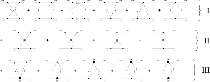
Figure 2: Dynamics of the Lorentz-invariant TPEP.

3 Comparison with the HB approach

The expressions for the Lorentz-invariant TPEP at N³LO is lengthy and will not be reproduced here (see [3, 5] instead). They are written in terms of Lorentz-invariant loop integrals which, due to the reasons mentioned in Sec.1, do not admit the naive HB expansion. Nevertheless, if one formally performs such unjustified expansion, one recovers all but three terms of the HB expressions [5]. These discrepancies come from two-loop diagrams of family II and affect mostly the central isovector component. Numerically, the difference is about 10% up to 3fm and decreases to 5–2% beyond that. It is not significant to the total central isovector component of the TPEP, since the contribution of family II is already fairly small [4]. The origin of such discrepancy still remains to be understood, and it might become relevant when more precision is asked for.

For now on we ignore the above mentioned discrepancies and concentrate only on the effect of expanding (HB) or not (RB) the Lorentz-invariant loop integrals. In Fig.3 we show the ratio of the HB over the RB versions of the TPEP, projected into two specific partial waves. The ${}^{1}G_{4}$ illustrates the general behavior of partial waves with total isospin $T=1$, which is similar to the LO+NLO terms in the HB expansion of the triangle integral (Fig.1). On the other hand, the partial waves with $T=0$, represented by ${}^{3}G_{5}$, are more sensitive to the HB expansion, with a discrepancy of 10–30% between 2 and 5fm, and increasing to almost 50% at $r=15$fm. This is due to the (isoscalar)$-$3(isovector) structure in those waves, each term having nearly the same magnitude. Although in Fig.3 we used the set EM 02 from Table 1, these qualitative results do not change with the choice of LECs.

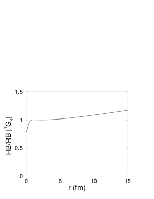
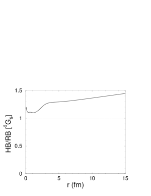
Figure 3: Ratios between HB and RB formulations of the TPEP, for ${}^{1}G_{4}$ and ${}^{3}G_{5}$ partial waves.

LEC	BM 00	Nij 03	EM 02	Set IV	Set $\eta$
$c_{1}$	$-0.81$	$-0.76$	$-0.81$	$-0.81$	$-0.81$
$c_{2}$	$8.43$	$3.20$	$3.28$	$3.28$	$3.28$
$c_{3}$	$-4.70$	$-4.78$	$-3.40$	$-3.20$	$-3.80$
$c_{4}$	$3.40$	$3.96$	$3.40$	$5.40$	$4.50$

LEC	FMS 98
$\bar{d}_{1}+\bar{d}_{2}$	$3.06$
$\bar{d}_{3}$	$-3.27$
$\bar{d}_{5}$	$0.45$
$\bar{d}_{14}-\bar{d}_{15}$	$-5.65$

Table 1: Values for the $\pi$N LECs, from several authors: BM 00 [8], Nij 03 [9], EM 02 [10], Set IV [11], and Set $\eta$ [12]. The numerical values of the couplings $d_{i}$’s, which have a small influence on NN observables, were taken from FMS 98 [13].

4 Phase shifts and deuteron properties

In Ref. [5] phase shifts for some peripheral waves ($F$, $G$, and $H$) were computed using the available $\pi$N LECs. The short-distance singularities were regulated with the same configuration-space cutoff used by the Argonne potentials [14], $[1-\exp(-cr^{2})]^{4}\times$TPEP, with $c=2.0{\rm fm}^{-2}$. That work has shown that the differences between the RB and HB results for these waves are negligible. That happens due to the large superposition of the one-pion exchange potential (OPEP), making the difference in Fig.3 hard to observe. More pronounced is the dependence of the phase shifts with the set of LECs. Fig.4 illustrates that with two selected partial waves.

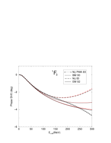
Figure 4: ${}^{1}F_{3}$ and ${}^{3}F_{4}$ phase shifts, using LECs from Table 1. For comparison, we also plot results from the Nijmegen partial wave analysis [15] (open circles).

Results for lower waves and deuteron properties were calculated in Ref. [12] using the renormalization method developed by the Granada group [16]. The central idea of the method is that the behavior of the potential at short distances fixes uniquely the form of the wave functions at the origin. A repulsive potential prevents the two particles to get close to each other, which causes the wave function to decrease exponentially in magnitude as $r$ goes to zero. In the attractive case, on the other hand, physical conditions have to be imposed to avoid the particles to collapse at the origin with infinite velocity. In the Granada method, this is achieved by demanding the wave function to satisfy specific boundary conditions at the origin. There the wave function is specified up to a phase, which is determined with an input of a physical quantity. For the generalized case of $N$ coupled channels, a potential diverging at the origin as ${\bf U}(r)\to{m_{N}{\bf C}_{n}/r^{n}}\,,$ with ${\bf C}_{n}$ a matrix of generalized Van der Waals coefficients, is diagonalized via an unitary matrix ${\bf G}$

$$m_{N}{\bf C}_{n}={\bf G}\,{\rm diag}(\pm R_{1}^{n-2},\dots,\pm R_{N}^{n-2})\,{\bf G}^{-1}\,,$$ (10)

with $R_{i}$ constants with length dimension. The plus (minus) sign corresponds to the case with a positive, attractive (negative, repulsive) eigenvalue. At short distances the solutions are given by ${\bf u}(r)\to{\bf G}\tilde{\bf u}$, where $\tilde{\bf u}$ is a column vector with components $u_{1,\pm}(r),\cdots,u_{N,\pm}(r)$. The attractive and repulsive cases behave respectively as

$$u_{i,-}(r) \to C_{i,-}\left(\frac{r}{R_{i}}\right)^{n/4}\sin\left[\frac{2}{n-2}\left(\frac{R_{i}}{r}\right)^{\frac{n}{2}-1}+\varphi_{i}\right]\,,$$ (11)

$$u_{i,+}(r) \to C_{i,+}\left(\frac{r}{R_{i}}\right)^{n/4}\exp\left[-\frac{2}{n-2}\left(\frac{R_{i}}{r}\right)^{\frac{n}{2}-1}\right]\,.$$ (12)

Here, $\varphi_{i}$’s are arbitrary short distance phases which in general depend on the energy. There are as many short distance phases as short distance attractive eigenpotentials. Orthogonality of the wave functions at the origin yields the relation

$$\sum_{i=1}^{N}\left[{u_{k,i}}^{*}u_{p,i}^{\prime}-{u_{k,i}^{\prime}}^{*}u_{p,i}\right]\Big{|}_{r=0}=\sum_{i=1}^{A}\cos(\varphi_{i}(k)-\varphi_{i}(p))\,,$$ (13)

where $A\leq N$ is the number of the short distance attractive eigenpotentials. The $\varphi_{i}$’s are fixed by low-energy (long-distance) input, which are the phase shifts close to threshold. The latter has a well-known low-energy expansion, the leading term being the inverse of the scattering “lengths”. For coupled channels with total (orbital) angular momentum $j$ ($j\pm 1$) the threshold behavior in the Stapp-Ypsilantis-Metropolis convention is

$$\bar{\delta}^{1j}_{j-1}\to-k^{2j-1}/\bar{a}^{1j}_{j-1}\,,\qquad\bar{\delta}^{1j}_{j+1}\to-k^{2j+3}/\bar{a}^{1j}_{j+1}\,,\qquad\bar{\epsilon}_{j}\to-k^{2j+1}/\bar{a}^{1j}_{j}\,.$$ (14)

Results for deuteron properties are given in Table 2. For the RB potential using Set IV, the asymptotic $D/S$ ratio $\eta$ is a prediction, which overshoots the $D$-state contribution. We noted that this can be remedied by slightly changing the chiral couplings $c_{3}$ and $c_{4}$ to reproduce the experimental value of $\eta$ (Set $\eta$).

Set	$\gamma({\rm fm}^{-1})$	$\eta$	$A_{S}({\rm fm}^{-1/2})$	$r_{d}({\rm fm})$	$Q_{d}({\rm fm}^{2})$	$P_{D}$
OPE	Input	0.02634	0.8681(1)	1.9351(5)	0.2762(1)	7.88(1)%
HB Set IV	Input	Input	0.884(4)	1.967(6)	0.276(3)	8(1)%
RBE Set IV	Input	0.03198(3)	0.8226(5)	1.8526(10)	0.3087(2)	22.99(13) %
RBE Set $\eta$	Input	0.02566(1)	0.88426(2)	1.96776(1)	0.2749(1)	5.59(1) %
NijmII	0.231605	0.02521	0.8845(8)	1.9675	0.2707	5.635%
Reid93	0.231605	0.02514	0.8845(8)	1.9686	0.2703	5.699%
Exp.	0.231605	0.0256(4)	0.8846(9)	1.971(6)	0.2859(3)	—

Table 2: Deuteron properties, for several NN potentials. [12].

A surprising result of the RB potential with Set $\eta$ is that the number of required low-energy inputs to renormalize the Schrödinger equation is significantly less than in the HB case, nearly a half (see Table II of Ref. [12]). This is a consequence of the different behavior of the RB potential near the origin, $V(r)\sim 1/r^{7}$, which resembles a relativistic Wan der Waals force, in contrast with the typical $1/r^{6}$ of the HB counterpart. There is also see a clear improvement in the deuteron properties and on the energy dependence of several phase shifts, some of them shown in Fig. 5. There are, however, some partial waves (${}^{1}S_{0}$, ${}^{1}D_{2}$, ${}^{3}F_{3}$, and ${}^{3}P_{2}$) where agreement with the Nijmegen partial wave analysis gets slightly worse. Compared to the HB, the ${}^{1}S_{0}$, ${}^{3}P_{2}$, $\epsilon_{2}$, ${}^{3}D_{3}$, and ${}^{3}G_{5}$ RB results are not satisfactory, but in other cases they are either consistent or better, remarkably for ${}^{1}D_{2}$, ${}^{3}P_{0}$, ${}^{3}P_{1}$, ${}^{3}D_{1}$, and $\epsilon_{1}$ [12].

Figure 5: Selected partial wave phase shifts using Sets IV and $\eta$, compared with the HB results (Set IV) and the Nijmegen partial wave analysis [15].

5 Summary

The program of constructing a nucleon-nucleon interaction based on the ideas of Becher and Leutwyler was presented. We pointed out the problem with the usual HB formalism in the one-nucleon sector and its consequences to the nucleon-nucleon system, namely, that it cannot account for the correct asymptotic description of the TPEP. If one performs a naive $1/m_{N}$ expansion of our results (which is not correct) one should, in principle, recover the HB expressions. In doing so, we noticed that there are three discrepant terms coming from two-loop dynamics. The origin of this discrepancy is not yet known and should be resolved if more precision calculations are demanded.

Considering only the effects of the $1/m_{N}$ expansion in the covariant loop functions, we showed that the HB and RB versions of the TPEP can have considerable differences, in particular the partial waves with total isospin $T=0$ in the physically interesting region between 2 and 5fm. However, this effect is barely noticeable in peripheral phase shifts, due to the large one-pion exchange contribution. More pronounced is their sensitivity to the $\pi$N LECs, in particular, $c_{3}$ and $c_{4}$.

To obtain the RB predictions for lower partial waves and deuteron properties, we used the renormalization method developed by the Granada group. We readjusted the LECs $c_{3}$ and $c_{4}$ to reproduce the asymptotic $D/S$ ratio (Set $\eta$), bringing other deuteron properties in agreement with experimental data and other potential model predictions. We also obtained an overall good agreement of the calculated phase shifts with the Nijmegen partial wave analysis, in a similar way as in the HB case. However, such agreement was obtained with significantly less counterterms (nearly a half) than the HB potential. That could be an advantage in determining the nucleon-nucleon LECs and bringing the RB potential into a form that could be eventually used in nuclear calculations.

- [1] T. Becher and H. Leutwyler, Eur. Phys. Journal C 9, 643 (1999); JHEP 106, 17 (2001).
- [2] S. Scherer, arXiv:0908.3425 [hep-ph].
- [3] R. Higa and M.R. Robilotta, Phys. Rev. C 68, 024004 (2003).
- [4] R. Higa, M. R. Robilotta, and C. A. da Rocha, Phys. Rev. C 69, 034009 (2004).
- [5] R. Higa, arXiv: nucl-th/0411046.
- [6] J. L. Friar, Phys. Rev. C 60, 034002 (1999).
- [7] N. Kaiser, R. Brockman, and W. Weise, Nucl. Phys. A625, 758 (1997).
- [8] P. Büttiker and U.-G. Meißner, Nucl. Phys. A668, 97 (2000).
- [9] M. C. M. Rentmeester, R. G. E. Timmermans, and J. J. de Swart, Phys. Rev. C 67, 044001 (2003).
- [10] D. R. Entem and R. Machleidt, Phys. Rev. C 66, 014002 (2002).
- [11] D. R. Entem and R. Machleidt, Phys. Rev. C 68, 041001(R) (2003).
- [12] R. Higa, M. Pavón Valderrama, and E. Ruiz Arriola, Phys. Rev. C 77, 034003 (2008).
- [13] N. Fettes, U.-G. Meißner, and S. Steininger, Nucl. Phys. A640, 199 (1998).
- [14] R. B. Wiringa, R. A. Smith, and T. L. Ainsworth, Phys. Rev. C 29, 1207 (1984); R. B. Wiringa, V. G. J. Stoks, and R. Schiavilla, Phys. Rev. C 51, 38 (1995).
- [15] V. G. J. Stoks, R. A. M. Klomp, M. C. M. Rentmeester, and J. J. de Swart, Phys. Rev. C 48, 792 (1993); Nijmegen on-line program, http://nn-online.org.
- [16] M. Pavón Valderrama, and E. Ruiz Arriola, Phys. Rev. C 74, 054001 (2006); Phys. Rev. C 74, 064004 (2006); Ann. Phys. 323, 1037 (2008).