Infrared Studies of Molecular Shocks in the Supernova Remnant HB 21:
II. Thermal Admixture of Shocked H₂ Gas in the South

Abstract

We present near- and mid-infrared observations on the shock-cloud interaction region in the southern part of the supernova remnant HB 21, performed with the InfraRed Camera (IRC) aboard AKARI satellite and the Wide InfraRed Camera (WIRC) at the Palomar 5 m telescope. The IRC 4 $\mu$m (N4), 7 $\mu$m (S7), and 11 $\mu$m (S11) band images and the WIRC H₂ $\upsilon=1\rightarrow 0$ S(1) 2.12 $\mu$m image show similar diffuse features, around a shocked CO cloud. We analyzed the emission through comparison with the H₂ line emission of several shock models. The IRC colors are well explained by the thermal admixture model of H₂ gas—whose infinitesimal H₂ column density has a power-law relation with the temperature $T$, $dN\sim T^{-b}dT$—with $n(\textrm{H}_{2})$ $\sim 3.9\times 10^{4}$ cm^-3, $b\sim 4.2$, and $N$(H${}_{2}\,;T>100\,\textrm{K})$ $\sim 2.8\times 10^{21}$ cm^-2. We interpreted these parameters with several different pictures of the shock-cloud interactions—multiple planar C-shocks, bow shocks, and shocked clumps—and discuss their weaknesses and strengths. The observed H₂ $\upsilon=1\rightarrow 0$ S(1) intensity is four times greater than the prediction from the power-law admixture model, the same tendency as found in the northern part of HB 21 (Paper I). We also explored the limitation of the thermal admixture model with respect to the derived model parameters.

1 Introduction

HB 21 (G89.0+4.7) is a large ($\sim 120^{\prime}\times 90^{\prime}$), middle-aged ($\sim 5000-7000$ yr, Lazendic and Slane 2006; Byun et al. 2006) supernova remnant (SNR) at a distance estimated to be from $\sim 0.8$ kpc to $\sim 1.7$ kpc (Leahy, 1987; Tatematsu et al., 1990; Byun et al., 2006). Based on its indented, shell-like appearance in the radio and the existence of nearby giant molecular clouds, it is thought to be interacting with a molecular cloud (cf. Fig. 1; Erkes and Dickel, 1969; Huang and Thaddeus, 1986; Tatematsu et al., 1990). The first direct evidence for this interaction was the detection of broad CO emission lines near the edge and the center of the remnant (Koo et al., 2001; Byun et al., 2006). The existence of such an interaction was further supported by the suggestion that evaporation of the cloud might be responsible for the enhanced thermal X-rays seen in the central part of the remnant (Leahy and Aschenbach, 1996).

We performed infrared imaging observations toward two localized positions in HB 21, where the broad CO emission lines were observed (Fig. 1), with two instruments: the InfraRed Camera (IRC, Onaka et al., 2007) aboard a Japanese satellite, AKARI (Murakami et al., 2007) and the Wide-field InfraRed Camera (WIRC, Wilson et al., 2003) on the Palomar 5 m Hale telescope. From the analysis of the northern part (“Cloud N”) data, we found that the mid-infrared diffuse features originated from shocked H₂ gas, with their excitation conditions well described by a thermal admixture of H₂ gas, whose infinitesimal H₂ column density has a power-law relation with the temperature $T$, d$N\sim T^{-b}dT$ (Shinn et al., 2009, hereafter Paper I). Such H₂ excitation conditions are consistent with the “ankle-like” energy level population diagram (i.e. a turn-up in population for higher energies, see Fig. 7), hitherto observed at the shock-cloud interaction regions (cf. $\S$ 1 of Paper I).

Here we present the analysis of the southern portion of HB 21 (“Cloud S”), following the method of Paper I. The near- and mid-infrared images ($\sim 2-13$ $\mu$m) we obtained show diffuse features around a shocked CO cloud. We analyze them as emission lines of H₂ gas in statistical equilibrium. We find the emission, as with the Cloud N case, to be well described with a power-law admixture model of thermal H₂ gas. We then discuss these results with physical pictures of the shock-cloud interaction.

2 Observations

We observed two specific regions (Cloud N and Cloud S in Fig. 1), where slow shocks ($\lesssim 20$ km s^-1) propagate into clouds of $n(\textrm{H}_{2})$ $\sim 10^{3}$ cm^-3 (Koo et al., 2001), using two different instruments: IRC (Onaka et al., 2007) aboard the AKARI satellite and WIRC (Wilson et al., 2003) on the Palomar 5 m telescope. The Cloud N data were analyzed in Paper I, and the Cloud S data are analyzed here. Details on the observations and reduction of the IRC and WIRC data are described separately, below.

2.1 AKARI IRC observations

AKARI is a satellite designed for both imaging and spectroscopy in the infrared (Murakami et al., 2007). The IRC is one of AKARI’s scientific instruments, which covers the wavelength range 2–30 $\mu$m and has a $\sim 10^{\prime}\times 10^{\prime}$ field-of-view for imaging. The IRC pointed-imaging observations for Cloud S were performed on 2007 Jun 3rd towards (RA, Dec) = ($20^{h}46^{m}07.80^{s}$, $+50^{\circ}02^{\prime}02.00^{\prime\prime}$) in J2000. IRC comprises three channels (NIR, MIR-S, and MIR-L), each of which has three band-pass filters for imaging. Among these, we employed four filters from NIR and MIR-S channels for the observations; the MIR-L channel was not used for observing Cloud S, due to lack of observing time. Table 1 lists the wavelength coverage and the imaging resolutions ($\Gamma$), together with pixel sizes in each channel.

Data reduction was the same as for the Cloud N data (cf. Paper I), except for flat-fielding; we used a different MIR-S flat, since the dark pattern seen in the channel changed around 2007 Jan 7th. We obtained the refined coadded image through the IRC Imaging Pipeline (v. 20070104 Lorente et al., 2007). Astrometric information was added to the coadded images, employing the 2MASS catalog (Skrutskie et al., 2006), with a matching tolerance of 1.5 pixels. The systematic errors ($\sim 2-5\%$) of the calibration were included in the error estimation, as done for the Cloud N data. Then, for the comparison between images from different bands, the pixel size was interpolated to $1^{\prime\prime}$ and the spatial resolution was smoothed to $\simeq 7.43^{\prime\prime}$. Point sources were removed applying the DAOPHOT package (Stetson, 1987) of IRAF making use of the simple-masking method. The final images for Cloud S are displayed in Figure 2.

2.2 Palomar WIRC H₂ observations

The WIRC observations were taken together with those of Cloud N (cf. Paper I). We carried out the H₂ $\upsilon=1\rightarrow 0$ S(1) 2.12 $\mu$m narrow-band filter imaging observation of Cloud S, centered at (RA, Dec) = (20h:46m:23.28s, $+49^{\circ}:54^{\prime}:16.72^{\prime\prime}$) in J2000, on the Palomar 5 m Hale telescope on 2005 August 29. The WIRC is equipped with a Rockwell Science Hawaii II HgCdTe 2K infrared focal plane array, covering a $8.7^{\prime}\times 8.7^{\prime}$ field of view with a $\sim 0.25^{\prime\prime}$ pixel scale. The WIRC field partially covered the IRC field, due to the mislocation of the WIRC observation center (cf. Fig. 2). The data reduction was also the same as that of Cloud N data. 50 dithered images of 30 sec exposure were obtained. We subtracted dark and sky background from each individual dithered frame and then divided by a normalized flat frame. Finally, the dithered frames were combined to produce the final image.

Astrometry was obtained by matching the positions of 13 field point-sources with those of 2MASS catalog sources, and the positions agreed within $\sim 0.3^{\prime\prime}$. Flux calibration was also done using the 2MASS catalog. We matched the magnitudes of 13 field point-sources with the corresponding $K_{s}$ magnitudes from the 2MASS catalog. Their correlation coefficient was 0.9956, and their ratio, $M_{WIRC}/M_{K_{s}}$, was $1.026\pm 0.011$. The systematic error ($\sim 14\%$) of the calibration was included in the error estimation. Point sources were removed using DAOPHOT. The full-width-at-half-maximum (FWHM) of these sources was found to be $\sim 1.1^{\prime\prime}$.

3 Results

The final images of IRC and WIRC are displayed in Figure 2, together with a ¹²CO $J=2\rightarrow 1$ 230.583 GHz (Koo et al., 2001) image for reference. The peak positions of the shocked S1 and S2 clouds, where broad ¹²CO $J=2\rightarrow 1$ lines were observed (Koo et al., 2001), are also indicated on the images.

3.1 Morphology

The IRC images (Fig. 2) show different features from band to band, as in Cloud N (Paper I). The N3 and N4 images are dominated by point sources, while the S7 and S11 images show similar diffuse features. They do not, however, look like bow shocks or planar shocks, unlike in Cloud N. Around the cloud S1, common diffuse features are seen in all the IRC images, although they are faint in the N3 image. However, there are no such diffuse features around the cloud S2. This is in contrast with Cloud N, where the shocked CO clouds have corresponding diffuse features in the IRC S7 and S11 bands; this is more interesting considering that the cloud properties observed from CO emission lines are similar for both clouds, S1 and S2 (Koo et al., 2001).

Higher extinction toward the cloud S2 than the cloud S1 does not seem to be the reason for the absence of diffuse IRC features around the cloud S2, since very high column density $N(\textrm{H})$$\,\gtrsim 10^{23}$ cm^-2 is required for the extinction to be effective at $\sim$ 10 $\mu$m (Draine, 2003). Recalling that H₂ emissions are the main source for the diffuse IRC features in the case of Cloud N (Paper I), this absence may be caused by the lack of H₂ gas around the cloud S2. The dissociation of H₂ by hot gas ($\gtrsim 10^{6}$ K) can be the reason, however it is unlikely since the X-ray emission is not strong around the cloud S2 (Byun et al., 2006). The X-ray flux ($0.1-2.4$ keV) of HB 21 is $31.8\times 10^{-10}$ erg s^-1 cm^-2 (Leahy and Aschenbach, 1996), and the cloud S2 locates $\sim 10^{\prime}$ away from the central X-ray emissions (Byun et al., 2006), which corresponds to a projected distance of $2-5$ pc. With a hydrogen nuclei density of $10^{4}$ cm^-3 and an attenuating column density of $10^{20}-10^{22}$ cm^-2, this distance corresponds to an effective ionization parameter, Log $\xi_{eff}$, ranging from $-4$ to $-7$, sufficiently small so that the effects of X-rays are negligible (Maloney et al., 1996). At the moment, it remains uncertain why such an absence of diffuse IRC features happens only to the cloud S2.

A diffuse, looplike feature with a diameter of $\sim 4^{\prime}$ is seen in the northern portion of the S7 and S11 images, however, it does not seem to be related with the shocked CO clouds S1 and S2. The ¹²CO $J=2\rightarrow 1$ map shows a similar looplike feature at 9.4 km s^-1 (Koo et al., 2001). Since the looplike feature looks similar in the IRC S7 and S11 bands, they may be generated by [Ar II] 6.99 $\mu$m and [Ne II] 12.8 $\mu$m emission lines, which are expected to show similar distributions in the shock-cloud interaction regions considering their ionization potentials (Neufeld et al., 2007); indeed, these lines have been frequently observed around SNRs (e.g.  Arendt et al., 1999; Oliva et al., 1999; Reach et al., 2002; Neufeld et al., 2007). Thermal emission from warm dust ($\gtrsim 100$ K) is another candidate. However, it seems unlikely because hot gas ($\gtrsim 10^{6}$ K)—the heat source for the warm dust—is not abundant around the cloud S1 (Fig. 1 of Byun et al., 2006).

The WIRC H₂ $\upsilon=1\rightarrow 0$ S(1) image only covered a small portion of the field of the IRC images because of the mislocation, but does include the cloud S1 (cf. Fig. 2). The H₂ image shows diffuse features around the cloud S1, similar to those seen in the IRC images. The similarity is more easily recognizable in Figure 3, which zooms into the area around the cloud S1. The RGB color image is made with N4 (blue), S7 (green), and S11 (red). Three elongated clumps, whose sizes are comparable with the FWHM of the IRC images ($\sim 7.4^{\prime\prime}$), are apparent. Overall, their colors are red-and-yellowish, although the southwestern part of the features shows a little bluish color. The filamentary features seen in the WIRC image have a similar overall morphology to those seen in the RGB image. They also surround the shocked CO cloud, S1 (cf. Fig. 2 and 3). This geometrical relationship thus suggests that the diffuse infrared features seen around the cloud S1 may also originate from shock excitation.

3.2 Quantitative Infrared Characteristics of the Shocked Gas

Since the cloud S2 shows no relevant feature in the IRC images and was not covered in the WIRC H₂ $\upsilon=1\rightarrow 0$ S(1) image, we analyzed the cloud S1 only. To quantify the infrared characteristics of the cloud S1, we measured its intensity in the IRC and WIRC images. The regions are outlined by the two concentric circles (see Fig. 3). The inner circle is the source region and the surrounding annular shell is the background region. To avoid any contamination during the measurement, possible point sources were excluded referring 2MASS point sources (Skrutskie et al., 2006); they are indicated as white circles with a red slash on Figure 3. The White circles with black shadings on the IRC images (Fig. 3) are bright point sources masked out during the data reduction (cf. $\S$ 2.1). Also, the northern part of the IRC images was additionally excluded since the WIRC image does not fully cover this region. The masked area is outlined by a white tetragon with a red slash.

Table 2 lists the measured intensities together with the IRC colors, N4/S7 and S7/S11. The IRC intensity is the strongest in S11, and decreases to shorter wavelength. Comparing with Cloud N, the S7 and S11 intensities are greater by a factor of 2–3 in the cloud S1. The colors are displayed as a point in Figure 4. The colors of the N2front in Cloud N are also displayed for comparison (cf. section 6.3.2). The cloud S1 and N2front have similar colors. The H₂ $\upsilon=1\rightarrow 0$ S(1) intensity was also extinction-corrected, as in Cloud N. We calculated the extinction factor to be $\sim 0.82$ ($A_{V}=1.8$ mag), derived from the extinction curve of “Milky Way, $R_{V}=3.1$” (Weingartner and Draine, 2001; Draine, 2003) with the foreground hydrogen nuclei column density, $N$(H)=$N$(H I)+2$N$(H₂)$=(3.5\pm 0.4)\times 10^{21}$ cm^-2, towards the center of HB 21 (Lee et al., 2001).

4 Radiation Source of the Shock-Cloud Interaction Features Observed in the AKARI IRC Bands

To interpret the infrared intensities and colors (Table 2), we must identify the radiation source of the features we see in the shock-cloud interactions. In Paper I, based on several arguments, we concluded that shocked H₂ gas was the most probable explanation for the interaction features observed in the IRC S7, S11, and L15 bands. In the similar manner, we here attribute the infrared features seen around the cloud S1 in the IRC N4, S7, and S11 bands to shocked H₂ gas.

Firstly, the similarity between the features seen in the IRC images and the Palomar WIRC H₂ $\upsilon=1\rightarrow 0$ S(1) image is also seen in the cloud S1 case. Although the IRC images are rather diffuse, they definitely show three elongated clumpy features, which similarly locate around the cloud S1 as in the H₂ $\upsilon=1\rightarrow 0$ S(1) image (Fig. 3 and $\S$ 3.1). At least, this suggests that the features seen in the IRC bands arise partly from H₂ emissions. Secondly, the same observational and theoretical arguments for H₂ emission, presented in Paper I, are valid over the IRC N4, S7, S11 bands ($\sim 3-13$ $\mu$m): (1) only the H₂ emission lines belong to the “lines of S and H₂($J_{\textrm{\footnotesize{up}}}>2$)” group can produce spatially similar features (Neufeld et al., 2007); (2) H₂ lines are the dominant emission from shocked molecular gas whose physical parameters are similar to the cloud S1 ($\upsilon_{s}$$=20$ km s^-1, $n(\textrm{H}_{2})$$=10^{4}$ cm^-3; Kaufman and Neufeld 1996).

We also considered other possible sources for the emission, presented in Paper I: fine structure ionic lines, thermal dust continuum, Polycyclic Aromatic Hydrocarbons (PAHs) bands, and synchrotron radiation. Again, these do not seem likely either, as we discuss below.

• Within the wavelength coverage of the IRC N4, S7, S11 bands, there are three strong ionic lines, [Fe II] 5.34 $\mu$m, [Ar II] 6.99 $\mu$m, and [Ne II] 12.8 $\mu$m, which have been observed in the shocked regions of SNRs (e.g.  Arendt et al., 1999; Oliva et al., 1999; Reach et al., 2002; Neufeld et al., 2007). The ionization potentials of these ions are 7.9 eV (Fe⁺), 15.8 eV (Ar⁺), and 21.6 eV (Ne⁺), respectively. From their case study on four SNRs, Neufeld et al. (2007) showed that the ions in shock-cloud interaction regions have two distinctive spatial distributions according to their ionization potential, $>13.6$ eV and $<13.6$ eV. Thus, in principle, the three ionic lines ([Fe II], [Ar II], and [Ne II]) can generate similar features in the IRC N4, S7, and S11 band images. However, the ions observed in the shock-cloud interaction regions have a low correlation with H₂ (Neufeld et al., 2007); indeed, such low correlations between [Fe II] and H₂ have been frequently observed around SNRs (e.g.  Oliva et al., 1999; Koo et al., 2007; Lee et al., 2009). For the case of cloud S1, which shows a good correlation between the diffuse IRC and the H₂ $\upsilon=1\rightarrow 0$ S(1) features (cf. section 3.1), it therefore seems that ionic lines from [Fe II], [Ar II], and [Ne II] are not responsible for the features we measured with AKARI.

• Thermal dust continuum is not likely responsible, either. To produce a correlated features through the IRC N4, S7, and S11 bands, the dust temperature should be higher than 500 K. In C-shocks, thought to be operating in the cloud S1, the dust temperature is below $\sim$50 K (Draine et al., 1983). In addition, to heat up the dust over 500 K, there should be hot gas ($\gtrsim 10^{6}$ K), well traced in X-rays, around the dust. However, no significant hot gas exists around the cloud S1 (Byun et al., 2006).

• PAHs are another candidate since they are ubiquitous and have strong, broad band features at 3.3, 6.2, 7.7, 8.6, 11.2, 12.7, and 16.4 $\mu$m (Tielens, 2008). However, in the similar ways presented in Paper I, they are not likely to be the source for the diffuse features seen in the IRC bands. PAHs are heated slowly and cool fast, thus it is hard to observe the shocked PAH emission above the background PAH emission (Tielens, 2008); although one case was claimed to detect the shocked PAH emission (Tappe et al., 2006), hitherto, such emissions have not been observed in shocks (van Dishoeck, 2004; Tielens, 2008).

• Synchrotron radiation is unlikely, as well, since no obvious correlation between the ¹²CO $J=2\rightarrow 1$ emission and the radio continuum was observed around the Cloud S (section 4.2 of Koo et al., 2001).

5 Comparison to Shock Models

To interpret the infrared intensities and colors (Table 2), we must model the excitation of the features. In Paper I, we concluded that shocked H₂ gas was the most probable explanation, based on several arguments. Among these, the clearest was the similarity of the diffuse features seen in the IRC and the WIRC H₂ $\upsilon=1\rightarrow 0$ S(1) images.

Hence, here we now analyze the band intensities as emission lines from shocked H₂ gas, which we calculate by applying several different shock models. These models are the same as in Paper I, except for the non-stationary model. This has been excluded since some bright H₂ emission lines which fall into the IRC N4 band are not listed in the published models (see Table 1 of Flower and Pineau des Forêts, 1999). Further descriptions of all these models are given in Paper I.

5.1 C-Shock: Isothermal H₂ Gas

It is known that the shocked H₂ gas behind a planar C-type shock can be approximated as an isothermal and isobaric slab of gas (Neufeld et al., 2006), in view of the H₂ excitation diagrams predicted for such shocks (e.g. Kaufman and Neufeld, 1996; Wilgenbus et al., 2000). Hence, we first calculate the expected IRC colors from the emission lines of isothermal H₂ gas. Figure 4 displays the modeled IRC colors from isothermal H₂ gas as open circles ($\circ$). Their trajectory moves from the lower-left corner to the upper-right corner as the temperature increases (i.e. becomes increasingly ’blue’). This is explained because pure rotational lines of H₂, which are dominant below a few 1000 K in the IRC bands, have shorter wavelengths for higher upper-levels. As $n(\textrm{H}_{2})$ increases, the populations are thermalized, approaching Local Thermodynamic Equilibrium (LTE).

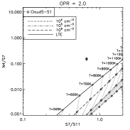
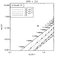
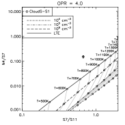
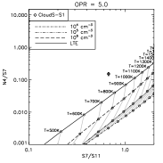
Figure 5: The IRC color-color diagrams for the cloud S1 with the expected colors for isothermal cases of various OPRs (cf. $\S$5.1). The rest of the graph is the same with Figure 4.

As Figure 4 shows, isothermal H₂ gas can not explain the observed IRC colors with any combination of $n(\textrm{H}_{2})$ and temperature. The ortho-to-para ratio (OPR) was also varied from 0.5 to 5, since the OPR is expected to be different from 3.0 in the interstellar clouds (Dalgarno et al., 1973; Flower and Watt, 1984; Lacy et al., 1994) and even in shocked gas (Timmermann, 1998; Wilgenbus et al., 2000). However, these variations are not able to reproduce the observed IRC colors (Fig. 5). The expected IRC colors at the same temperature vary according to the adopted OPR; however, the locus of the IRC colors do not differ much from the OPR=3.0 case, that is shown in Figure 5.

A similar result was already found for the Cloud N, and it is consistent with the H₂ level populations displaying an ankle-like curve (see Fig. 7). The critical density of an H₂ line transition increases as the energy level of the upper state increases (cf. Le Bourlot et al., 1999); hence, isothermal H₂ gas can only produce either a straight line (LTE) or a knee-like curve (non-LTE, see Fig. 1 in Paper I) in the population diagram, neither of which are observed. Therefore, the cloud S1 also has an ankle-like H₂ population.

This ankle-like population can be understood by the morphology of the diffuse H₂ $\upsilon=1\rightarrow 0$ S(1) features. These features are filamentary and surround the shocked CO cloud (cf. Fig. 2 and 3). Hence, if they are generated by shocks propagating into the cloud S1, a range of shock velocities are expected. Since the postshock temperature of C-shock is proportional to the shock velocity as $\upsilon_{s}$^1.35 (Neufeld et al., 2006), a moderate difference in $\upsilon_{s}$ may result in a range of temperature in the shocked H₂ gas. However, this explanation may not be valid, because the same population was also found for the N2front of Cloud N, whose appearance is so planar that little difference in shock speed is expected (Paper I).

5.2 C-Shock: Power-law Distribution of H₂ Gas Temperature

Figure 4 also displays the IRC colors calculated from the admixture model for H₂ gas, as filled circles ($\bullet$). As can be seen, it can reproduce the observed IRC color ratios with an appropriate combination of $n(\textrm{H}_{2})$ and $b$. The derived parameters are listed in Table 3. $N$(H${}_{2}\,;T>100\,\textrm{K})$ is determined by scaling the modeled IRC intensity for the derived $n(\textrm{H}_{2})$ and $b$ to meet the observed IRC intensity. The detail contributions of H₂ line emission to IRC bands for these parameters are listed in Table 4. The “Weight” column of Table 4 lists the weighting factor for each line to the IRC band contribution. For example, the S11 band intensity can be calculated as follows.

$$\frac{I_{S11}(\textrm{H${}_{2}$})}{\textrm{MJy sr${}^{-1}$}}=\frac{0.610\,I[\textrm{H${}_{2}$}\,S(2)]+0.921\,I[\textrm{H${}_{2}$}\,S(3)]}{10^{-4}\,\textrm{erg s${}^{-1}$ cm${}^{-2}$ sr${}^{-1}$}}$$ (1)

As Table 4 shows, the pure-rotational H₂ emission lines are dominant in all IRC bands. Since the N4 band, in contrast to the L15 band used for Cloud N, is used for the color-color diagram of the S1 cloud (Fig. 4), the contribution from several higher-level emission lines, S(7)–S(11), was also included, while that from the S(1) 17 $\mu$m emission line was not applied (cf. Table 4 of Paper I). We here note that the model parameters for N2front derived from the N4/S7 vs. S7/S11 color-color diagram (Fig. 4), $b\sim 4$ and $n(\textrm{H}_{2})$$\sim 4\times 10^{4}$ cm^-3, are both larger than those from the S7/S11 vs. S11/L15 diagram (Paper I), $b\sim 3$ and $n(\textrm{H}_{2})$$\sim 2\times 10^{3}$ cm^-3. We discuss this issue further in section 6.3.2.

In addition, since ¹²CO $v=1-0$ 4.6 $\mu m$ emission lines have been observed in shocked gas (e.g. Rosenthal et al., 2000) and fall into the IRC N4 band coverage, we assessed their contribution to the band, for the power-law thermal admixture model with $b=4.0$ and $5.0$, referring the assessment of Neufeld and Yuan (2008). We used the CO vibrational energy state of Balakrishnan et al. (2002) and the CO vibrational transition rate of Chandra et al. (1996). We adopted the collisional rate coefficients for the excitation of CO vibrational transitions by H (Balakrishnan et al., 2002) and by He (Cecchi-Pestellini et al., 2002). For excitation by H₂, we adopted the equations [7] and [8] of Thompson (1973) with the parameter $A$ of 68, the laboratory measurement of Millikan and White (1963). Unlike the excitation of H₂ gas, we included H as a collisional partner for the CO vibrational excitation since H excites CO vibrational levels ($\upsilon>0$) more efficiently than He and H₂. H excites the H₂ pure rotational levels ($\upsilon=0$) less efficiently than He and H₂ (Le Bourlot et al., 1999), hence including H as a collisional partner in the excitation of H₂ gas makes negligible effects on the predicted IRC band intensity, where the pure rotational lines are dominant (cf. Table 4).

Figure 6 displays the results. The fractional abundance of atomic hydrogen to molecular hydrogen, $N$(H I)/$N(\textrm{H}_{2})$, was varied as 0, 0.01, 0.1, and 1.0, while that of CO was fixed as $10^{-4}$. As with the H₂ vibrational states, those of CO also have higher collisional coefficients for a collision with atomic hydrogen than with He or H₂; hence, Figure 6 shows a sensitive dependence on the ratio, $N$(H I)/$N(\textrm{H}_{2})$. In the range of $n(\textrm{H}_{2})$=$10^{3}-10^{6}$ cm^-3, the contribution to the IRC N4 band is less than 0.1, hence negligible. Furthermore, a robust simulation expects that ¹²CO $v=1-0$ emission lines are much weaker than those of H₂ in C-shocks of preshock H₂ densities $n(\textrm{H}_{2})$$=10^{4}-10^{6}$ cm^-3 and shock velocities $\upsilon_{s}$=20–40 km s^-1 (Kaufman and Neufeld, 1996).

The derived parameters, except the power-law index $b$, are a little higher than those previously determined towards several SNRs, where interaction with nearby molecular clouds is occurring. The density, $n(\textrm{H}_{2})$=(3.9${}_{-1.2}^{+2.1}$)$\times 10^{4}$ cm^-3, is a few times higher than the value, derived from Large Velocity Gradient (LVG) analysis of CO data for HB 21, of $n(\textrm{H}_{2})$$=7.0\times 10^{3}$ cm^-3 by Koo et al. (2001). The column density we derived, $N$(H${}_{2}\,;T>100\,\textrm{K})$=(2.8${}_{-0.5}^{+0.2}$)$\times 10^{21}$ cm^-2, is similarly higher than that derived towards shock-cloud interaction regions in four other SNRs (W 44, W 28, 3C 391, and IC 443), $N(\textrm{H}_{2})$$=(2.8-8.9)\times 10^{20}$ cm^-2. The latter values were determined from a two-temperature LTE fitting of pure-rotational H₂ spectra with varying OPRs (Neufeld et al., 2007). Our derived $b$-value of 4.2${}_{-0.1}^{+0.1}$ falls into the middle of the range, 3.0–6.0, found by Neufeld and Yuan (2008). These authors found the IRAC color ratios to be well explained with this range of power-law index $b$, analyzing Spitzer IRAC observations towards the SNR IC 443. From these three parameters derived—$n(\textrm{H}_{2})$, $N$(H${}_{2}\,;T>100\,\textrm{K})$, and $b$—we also determined the model prediction for the H₂ $\upsilon=1\rightarrow 0$ S(1) intensity, (1.5${}_{-0.3}^{+0.5}$)$\times 10^{-6}$ erg s^-1 cm^-2 sr^-1. It is about a factor of four smaller than the observed value (see Table 2 and 3). In contrast, for Cloud N the excess was found to be a factor of $17-33$ (Paper I). We discuss these results further in $\S$6.

Finally, we visualized the population state of the cloud S1, derived from the IRC color-color diagram, in Figure 7 (left). The pure-rotational levels which contribute to the IRC bands are designated with filled circles. Also, the upper level of H₂ $\upsilon=1\rightarrow 0$ S(1) emission line is designated with a filled triangle; its population derived from the observed H₂ $\upsilon=1\rightarrow 0$ S(1) intensity, extinction corrected, is designated with a grey filled triangle with an error bar. The diagram shows a severe deviation of $\upsilon>0$ levels from $\upsilon=0$ level, it thus seems that the two temperature LTE fitting, a model usually applied for shocked H₂ gas (e.g. Rho et al., 2001; Giannini et al., 2006), does not properly describe the population state of the cloud S1, even with varying OPR. This is caused by the low $n(\textrm{H}_{2})$ of the cloud S1, $\sim 4\times 10^{4}$ cm^-3, which is much lower than the critical densities for ro-vibrational H₂ lines, $\gtrsim 10^{8}$ cm^-3 (Le Bourlot et al., 1999). We also note that this type of $\upsilon>0$ states population may not be easily recognizable with near-infrared ground observations, since only the population for a few lowest-$J$ levels of the $\upsilon>0$ states can be deduced due to the atmospheric absorption (e.g. Burton et al., 1989; Giannini et al., 2006). Hence, for an exact derivation of the H₂ level population, we must cover full range of $\sim 2-30$ $\mu$m at once as in Rosenthal et al. (2000), and space observatories are ideal and mandatory in this sense.

5.3 Partially Dissociative J-shock

As Figure 8 shows, a partially dissociating jump-shock model does not reproduce the observed color of the cloud S1. The observed color might appear to lie on a model extension to very high pressure, higher than $P=10^{11}$ cm^-3 K; however, this is implausible. From their CO observations, Koo et al. (2001) derived $n(\textrm{H}_{2})$$=7.0\times 10^{3}$ cm^-3 and $\upsilon_{s}$$\lesssim 20$km s^-1 for the cloud S1. These give a postshock pressure of $\sim 10^{8}$ cm^-3 K, which is more than $10^{3}$ times lower than the above limit. A pressure enhancement can occur for the collision between molecular clumps and radiative shells of a remnant (e.g. Moorhouse et al., 1991; Chevalier, 1999); however, it is only about a factor of 20. Insufficient cooling time cannot solve the disagreement between the observed and modeled colors, either. If the postshock H₂ had not cooled as low as a few hundred K, then the modeled IRC colors move towards the upper-right direction in the color-color diagram (Fig. 4) to bluer colors. This was not observed. Overall, a partially dissociative J-shock does not seem to be a suitable model to explain the observed IRC colors.

6 Discussion

The observed color ratios were only reproduced by the thermal admixture model, as was the case for Cloud N (Paper I). Hence, we here discuss the derived parameters from this model, based on pictures for the shock-cloud interactions, as proposed in Neufeld and Yuan (2008) and in Paper I. We also note here that we assumed the OPR=3.0 since no OPR information is available for the cloud S1; hence, the derived parameters can be changed according to the adopted OPR value.

6.1 Nature of Molecular Shocks Seen in the Infrared

Diffuse infrared features surround the shocked CO cloud S1 (see Fig. 2 and 3). For instance, the H₂ $\upsilon=1\rightarrow 0$ S(1) image shows several filamentary features, as if excited by shocks propagating into the cloud core. These may represent distinctive planar shocks, each with different speed. From the previous observations toward SNR molecular shock regions, the H₂ level population diagram has been shown to have an ankle-like curve (cf. Fig. 7). For planar C-shocks to explain such populations, it generally requires two components, whose shock velocities are $\sim 10$ and $\sim 30-50$ km s^-1, with comparable amounts of $N(\textrm{H}_{2})$ (cf.  Hewitt et al., 2009). Hence, the filamentary features seen in the H₂ $\upsilon=1\rightarrow 0$ S(1) image may originate from such a mixture of planar C-shocks. However, the possibility that the individual filamentary feature bears the ankle-like population still remains, since such a property was seen in a very planar filamentary feature of Cloud N (N2front).

Neufeld and Yuan (2008) showed that the $b$ values they obtained, $\sim 3.0-6.0$, can be explained by paraboloidal bow shocks, which are geometrical summations of planar C-shocks (see Fig. 9). In their picture, a paraboloidal bow shock, where H₂ survives the shock (i.e. T$\lesssim 4,000$ K), has a power-law index $b\sim 3.8$. If some slower bow-shocks which do not reach 4000 K are then spatially averaged together, a value for $b$ of $\gtrsim 3.8$ is generated.

The value $b$ for the cloud S1 was determined to be 4.2${}_{-0.1}^{+0.1}$, which falls into the range derived for bow shocks, $b\gtrsim 3.8$. However, as discussed in Paper I, bow shocks should have been observed in the H₂ $\upsilon=1\rightarrow 0$ S(1) image, if any, since the expected shock width for a planar C-shock propagating into preshock gas of $n(\textrm{H}_{2})$ $\sim 10^{4}$ cm^-3 is $\sim 10^{16}$ cm (Draine et al., 1983), comparable to the spatial resolution in the image, $\sim 1.1^{\prime\prime}$ (cf. $\S$ 2.2) $\sim(1.3-2.8)\times 10^{16}$ cm for the distance of $\sim 0.8-1.7$ kpc (Leahy, 1987; Tatematsu et al., 1990; Byun et al., 2006). This absence of bow shock features can be explained by the viewing angle. If we consider the circular and filamentary appearance of the diffuse H₂ features around the cloud S1, it may be possible that a single paraboloidal bow-shock is being viewed along its symmetry axis, producing the circular feature seen in Figure 3. In this case, our result fit with the bow shock picture of Neufeld and Yuan (2008), when seen face-on.

This bow shock picture has a difficulty in achieving a steady state for the shock, however. It assumes a steady state planar C-shock at every point of the bow. Through the C-type shock, the $n(\textrm{H}_{2})$ can be increased up to a factor of ten (e.g. Timmermann, 1998; Wilgenbus et al., 2000). Thus, $n(\textrm{H}_{2})$ at the upstream of the bow would be $\sim$ [$n(\textrm{H}_{2})$ at downstream]$\times 0.1\sim[4\times 10^{4}]\times 0.1\sim 4\times 10^{3}$ cm^-3 (cf. Table 3 and Fig. 9). Also, the preshock gas velocity into the shock is known to be $\sim 20$ km s^-1 from CO observations (Koo et al., 2001). For these preshock density and shock velocity, the time required to achieve a steady shock is known to be $\sim 10^{4}$ yr from the study on the early stage of shock generation (Flower and Pineau des Forêts, 1999). This time seems to be long for the bow shock around the cloud S1 to be in a steady state, considering the estimated age of HB 21, $\sim 5000-7000$ yr (Lazendic and Slane, 2006; Byun et al., 2006), together with the location of the cloud S1 near the edge of the remnant (Fig. 1); we here note that the remnant may be older than 5000-7000 yr, estimated at the distance of 0.8 kpc, since the distance is uncertain, $\sim 0.8-1.7$ kpc (Leahy, 1987; Tatematsu et al., 1990; Byun et al., 2006).

In Paper I, we conjectured that a shocked clumpy interstellar medium (ISM) exists (cf. Fig. 9), based on the similar $b$ values of the N2front and N2clump regions and on the cyclodial (cuspy) feature seen in the N2clump region, together with numerical simulations (Nakamura et al., 2006; Shin et al., 2008). If this picture also holds for the S1 cloud, the shocked clump must be unresolved in the WIRC H₂ $\upsilon=1\rightarrow 0$ S(1) image, since the H₂ features around this cloud do not show any cycloidal features. However, even though this is the case, the absence of the wriggle expected for shock fronts propagating a clumpy ISM (e.g. Patnaude and Fesen, 2005) still remains as an issue (cf. Fig. 3)—the wriggle is generated by shocks propagating further through a lower density medium, and vice versa. This wriggle can be unresolved in the H₂ $\upsilon=1\rightarrow 0$ S(1) image if its scale is small enough ($\lesssim 10^{16}$ cm). However, it is uncertain whether the cycloidal feature would be maintained under such a small scale.

As noted in section 3.2, the N4/S7 vs. S7/S11 colors of the cloud S1 and N2front are similar (cf. Fig. 4). This is intriguing considering that they are physically unrelated. Their morphologies seen in H₂ $\upsilon=1\rightarrow 0$ S(1) images are also similar, i.e. filamentary, although their sizes show a few factors of difference (cf.  Paper I and Fig. 3). These similarities suggest that the cloud S1 and N2front share similar shock conditions. The interstellar ultraviolet radiation field may contribute to this similarity; however, a more robust study is required.

6.2 H₂ $\upsilon=1\rightarrow 0$ S(1) intensity

We estimated the H₂ $\upsilon=1\rightarrow 0$ S(1) intensity of the cloud S1 for the derived model parameters—$n(\textrm{H}_{2})$, $b$, and $N$(H${}_{2}\,;T>100\,\textrm{K})$—from the mid-infrared IRC colors. It is about four times weaker than the observed intensity (Table 2 and 3). This discrepancy is less severe than the Cloud N case, which shows a factor of 17–33 difference (Paper I). However, the amount of excited gas, $N(\textrm{H${}_{2}$};v=1,J=3)$, required to compensate for the difference is $\sim 10^{14}$ cm^-2 in both cases (cf. Fig. 7).

In Paper I, we discussed two possible reasons for the discrepancy. Firstly, the existence of additional H₂ gas, whose temperature and density are both high, but whose column density is low enough to have negligible effect on the mid-infrared line intensities. For example, to compensate for a deficiency of $N(v=1,J=3)\sim 10^{14}$ cm^-2, we need an additional amount of H₂ gas of $N(\textrm{H}_{2})$ $\sim 10^{16}$ cm^-2 in LTE with $T\sim 2000$ K. A compact, unresolved shocked cloud is a candidate for such additional H₂ gas.

The second explanation given was the omission of collisions with hydrogen atoms, which are effective in exciting the vibrational states of H₂ (cf.  Neufeld and Yuan, 2008). The cross section for excitation of H₂ by H is several orders of magnitude greater for rovibrational transitions than it is for pure rotational transitions (see Table 1 and Figure 1 in Le Bourlot et al., 1999). Hence, with only a small fraction of H, $n(\textrm{H})$/$n(\textrm{H}_{2})$$\sim 0.025$, the rovibrational transition can be dominated by collisions with H, rather than with H₂, in the temperature range 300–4000 K. Indeed, such a fraction of atomic gas is expected in interstellar clouds with $n(\textrm{H}_{2})$ $\gtrsim 10^{3}$ cm^-3 (see Table 1 and Figure 1 in Snow and McCall, 2006), as well as in theoretical models for shock waves that are fast enough to produce H₂ at temperatures of a few thousand K (e.g. Wilgenbus et al., 2000).

6.3 Limitation of the Thermal Admixture Model

6.3.1 H₂ Column Density $N(\textrm{H}_{2})$

In section 5.2, we mentioned that the column density $N$(H${}_{2}\,;T>100\,\textrm{K})$ of the cloud S1 is a few times higher than those of other SNRs (W 44, W 28, 3C 391, and IC 443). The former is $N$(H${}_{2}\,;T>100\,\textrm{K})$=(2.8${}_{-0.5}^{+0.2}$)$\times 10^{21}$ cm^-2, while the latter are $N(\textrm{H}_{2})$$=(2.8-8.9)\times 10^{20}$ cm^-2 (Neufeld et al., 2007). This seems unreasonable considering that the $n(\textrm{H}_{2})$ of the cloud S1, (3.9${}_{-1.2}^{+2.1}$)$\times 10^{4}$ cm^-3, is lower than that of IC 443, $\sim 10^{7}$ cm^-3 (Neufeld and Yuan, 2008). However, there is one important point to note before the comparison: those H₂ column densities are expectations estimated using different methods.

The total column density of H₂ gas at a few 100 K is mainly determined by the values of $\upsilon=0$ $J=0,1$ levels, since other levels have much lower populations (cf. Fig. 7). However, we cannot obtain the column densities of these levels directly from emission lines, because no transition to a lower state is allowed; therefore, we must estimate the column densities of $J=0,1$ levels from the observed column densities of $J>1$ levels. The different methods used for this estimation causes the discrepancy between the cloud S1 and IC 443, mentioned above, as we discuss below.

The $N$(H${}_{2}\,;T>100\,\textrm{K})$ of the cloud S1, (2.8${}_{-0.5}^{+0.2}$)$\times 10^{21}$ cm^-2, is estimated by applying the thermal admixture model to the observed IRC intensities, while the $N(\textrm{H}_{2})$ of IC 443, $\sim 5.0\times 10^{20}$ cm^-2, was estimated with two temperature LTE fitting with varying the OPR (Neufeld et al., 2007). If we estimate the $N(\textrm{H}_{2})$ of the cloud S1 using the same two-temperature LTE fitting, we would obtain a lower values. Figure 7 (top-right) displays the result of such fitting. The fitting was applied only to the H₂ levels whose emission lines contribute to the IRC bands (cf. Table 4), and returned a column density of $\sim 7.3\times 10^{19}$ cm^-2. This is about seven times less than IC 443, and now does not cause the discrepancy mentioned above.

Also, this column density is about 40 times smaller than the estimation using the thermal admixture model. This difference stems from the fact that the thermal admixture model does not estimate the column densities of $J=0,1$ with a linear extrapolation in the population diagram as the LTE fitting does (cf. Fig. 7); it estimates the column densities with a curved population, defined by the equation $dN\sim T^{-b}dT$ (100 K $\leq T\leq$ 4000 K). Such a difference is smaller when longer wavelength IRC bands are used for the column density estimation. Figure 7 (bottom-right) shows the results of the two temperature LTE fitting for the population of the N2front, determined using the IRC S7, S11, and L15 bands (Paper I); the result shows a column density of $\sim 7.5\times 10^{19}$ cm^-2, which is about 3.3 times smaller than the estimation using the thermal admixture model, $\sim 2.5\times 10^{20}$ cm^-2 (Paper I). This trend is reasonable since the longer wavelength IRC bands determine the level populations of lower-$J$ states in $\upsilon=0$, which results in a less severe extrapolation for the column densities, $N(J=0,1)$.

6.3.2 H₂ Density $n(\textrm{H}_{2})$ and power-law index $b$

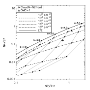
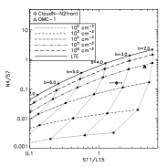
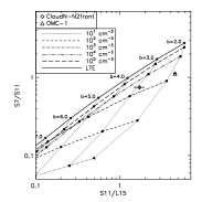
Figure 10: The IRC color-color diagram for N2front and Orion Molecular Cloud-1: (leftmost) N4/S7 versus S7/S11, (middle) N4/S7 versus S11/L15, and (rightmost) S7/S11 versus S11/L15. The grids are the expected colors from the thermal admixture model (cf. section 5.2). Depending on which IRC bands are used for the color-color diagram, the obtained parameters, $b$ and $n(\textrm{H}_{2})$, are different for each data point; the shorter-wavelength bands return the higher-$b$ and higher-$n(\textrm{H}_{2})$ (cf. N4/S7 vs. S7/S11 and S7/S11 vs. S11/L15 diagrams). See section 6.3.2 for detail.

To compare the N4/S7 and S7/S11 colors of the cloud S1 with those of N2front in Cloud N (Fig. 4), we further determined the N4 intensity of N2front, which was not measured in Paper I because of strong point source contamination. In order to remove this contamination, we additionally masked point-source dominated areas seen in the N4 band. Table 5 shows the measured intensities. Since some areas are additionally masked unlike Paper I, the intensities of S7, S11, and L15 are a little different from those listed in Paper I; however, the colors S7/S11 and S11/L15 are almost unchanged (cf. Fig. 7 in Paper I and Fig. 10). Therefore, we think the point-source masking was done properly.

Figure 10 shows that the model parameters, $b$ and $n(\textrm{H}_{2})$, obtained for N2front depends on which IRC bands are used for the color-color diagram. The diagram of shorter wavelength bands (N4, S7, S11; Fig. 10 leftmost) returns larger-b and larger-$n(\textrm{H}_{2})$ values than the diagram of longer wavelength bands (S7, S11, L15; Fig. 10 rightmost), and the diagram of N4/S7 vs. S11/L15 (Fig. 10 middle) returns the middle values of the former two diagrams’. This inconsistency may be caused by the intrinsic property of shocked H₂ gas. In other words, the whole level population of shocked H₂ gas may not be fully described by the power-law thermal admixture model with only one set of $b$ and $n(\textrm{H}_{2})$.

To check this possibility, in Figure 10, we overplotted the IRC colors of Orion Molecular Cloud-1 (OMC-1), where extensive emission lines of shocked H₂ gas were observed over $2.5-30$ $\mu$m (Rosenthal et al., 2000). The OMC-1 emissions were adjusted to experience the same extinction with HB 21, to be placed in the model grid for N2front. Interestingly, OMC-1 also shows the same trend for the model parameters, $b$ and $n(\textrm{H}_{2})$, as the case for N2front. This suggests that the variations of $b$ and $n(\textrm{H}_{2})$ are needed for the thermal admixture model to describe the whole level population of shocked H₂ gas. No significant variation of $b$ was seen in the SNR IC 443, where the thermal admixture model was applied first (Neufeld and Yuan, 2008). It may be caused by the narrow wavelength coverage of the bands they used (Spitzer IRAC; $\sim 3-8$ $\mu$m), which missed the longer wavelength information we used. We here note that the model parameters—$b$ and $n(\textrm{H}_{2})$—must be obtained from the same band images for their comparison between different shocked regions, since the parameters are likely dependent on the wavelength.

7 Conclusion

We have observed a shock-cloud interaction region in the SNR HB 21 at near- and mid-infrared wavelengths, with the WIRC at the Palomar telescope and the IRC aboard the AKARI satellite. The IRC N4, S7, and S11 band images and the WIRC H₂ $\upsilon=1\rightarrow 0$ S(1) image reveal similar diffuse features, which surround the shocked CO cloud S1. However, there are no infrared diffuse features seen around another shocked CO cloud S2. Lack of shocked H₂ gas may cause this absence, but why it happens only for the cloud S2 is uncertain.

We found that the IRC colors of the cloud S1 are well explained by an admixture model of H₂ gas temperatures, whose infinitesimal column density varies as $dN\sim T^{-b}dT$. Three physical parameters—$n(\textrm{H}_{2})$, $b$, and $N$(H${}_{2}\,;T>100\,\textrm{K})$—were derived from this thermal admixture model (cf. Table 3). These can be understood with multiple planar C-shocks whose velocities are different. Alternatively, the derived $b$ value ($\sim 4.2$) can be understood through a bow shock picture, if we are looking at a single bow shock along the symmetry axis. However, this picture has a difficulty in achieving a steady state. A shocked clumpy ISM picture, conjectured in Paper I, remains as a possible explanation, but the absence of the wriggle, expected for shock fronts propagating a clumpy medium, in the filamentary features seen in H₂ $\upsilon=1\rightarrow 0$ S(1) image remains as an issue. The model parameters, $b$ and $n(\textrm{H}_{2})$, obtained for the cloud S1 and N2front (cf. Fig. 4) are very similar, which means that these clouds share similar shock conditions.

We also compared the observed H₂ $\upsilon=1\rightarrow 0$ S(1) intensity to that predicted from the power-law admixture model. It is about four times greater. This excess might be caused by either an additional component of hot, dense H₂ gas (which has low total column density), or by the omission of collisions with hydrogen atoms in the power-law admixture model (which results in an under-prediction of the near-IR line intensity).

The limitation of the thermal admixture model is explored with respect to the derived model parameters. The $N(\textrm{H}_{2})$ estimation of the model shows a smaller difference with those of two temperature LTE fitting, when longer wavelength IRC bands are used for the determination of model parameters. Investigating the infrared colors of N2front and OMC-1 in the four IRC bands (N4, S7, S11, and L15), we found that the thermal admixture model cannot describe the whole H₂ level population with only one set of $b$ and $n(\textrm{H}_{2})$; the shorter wavelength bands returns higher-$b$ and higher-$n(\textrm{H}_{2})$. This tells we must use the same bands in determining the model parameters, for the comparisons of the shocked H₂ gas’ properties.

Figure 1: Regions observed by AKARI. The IRC pointing-observation regions (“Cloud N” and “Cloud S”) are overlaid as two boxes ($\sim 10^{\prime}\times 10^{\prime}$) on the 1420 MHz radio continuum image of HB 21, obtained by using the synthesis telescope at the Dominian Radio Astrophysical Observatory. The Palomar WIRC observations were performed toward a similar region. In this paper, we present the Cloud S data. The Cloud N data were presented in Shinn et al. (2009). The 1420 MHz radio continuum image is kindly provided by T. L. Landecker.

Figure 2: The AKARI IRC and Palomar WIRC images of Cloud S. See Table 1 for the band definitions for the IRC images. (upper-panels) IRC N3, N4, and S7 band images. (lower-panels) IRC S11 band, ¹²CO $J=2\rightarrow 1$ 230.583 GHz (Koo et al., 2001), and H₂ $\upsilon=1\rightarrow 0$ S(1) 2.122 $\mu$m images. The peak positions (“S1” and “S2”), where broad CO molecular lines were observed, are indicated with a ‘+’ over all images (cf. Koo et al., 2001). Bright point-sources were masked out, shown by the white circles in the IRC images. The center position of the WIRC H₂ $\upsilon=1\rightarrow 0$ S(1) image was mislocated, hence the partial image is shown here. A scale bar at the upper-left corner shows $1^{\prime}$.

Figure 3: The IRC RGB image (left) and the WIRC H₂ $\upsilon=1\rightarrow 0$ S(1) image (right) of the cloud S1. The RGB image is composed of S11 (R), S7 (G), and N4 (B) band images, i.e. 11 $\mu$m + 7 $\mu$m + 4 $\mu$m. All colors scale linearly, and fully cover the dynamic range of the diffuse features. The annular regions selected for the intensity measurement are indicated as two concentric white circles. The inner circle is the source region and the outer annular region is the background region. Circular areas around possible point sources were excluded during the intensity measurement to avoid possible contamination. These areas are indicated as white circles with a red slash. Bright point-sources are masked out, and their positions are indicated by white circles with black shading. For the comparison between the IRC and WIRC intensity, a tetragonal region is excluded from the IRC images. The cross (‘+’) indicates the peak positions (“S1”), where broad CO molecular lines were observed, as in Figure 2.

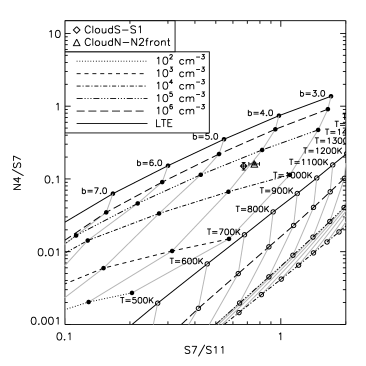
Figure 4: The IRC color-color diagram for the cloud S1, with the colors of the N2front in Cloud N plotted for comparison (cf. section 6.3.2). The axes represent the ratio of the intensities in the corresponding IRC bands. The data points are shown by the diamond (S1) and triangle (N2front). The expected colors for both isothermal ($\S$5.1) and power-law-thermal ($\S$5.2) cases are indicated as open circles ($\circ$) and filled circles ($\bullet$), respectively. OPR=3.0 is assumed for both cases. The different types of black lines connect points of equal $n(\textrm{H}_{2})$ and the LTE case. The grey solid lines connect points of equal power-law index ($b$) or equal temperature ($T$). The values for the power-law index and temperature are also indicated.

Figure 6: Fractional contribution of ¹²CO $v=1-0$ emission lines to the IRC N4 band as a function of $n(\textrm{H}_{2})$. Filled circles and open circles are for $b=4.0$ and $b=5.0$, respectively. $X_{H}$ is the fractional abundance of atomic hydrogen to molecular hydrogen, $N$(H I)/$N(\textrm{H}_{2})$. The fractional abundance of CO to H₂ is assumed to be $10^{-4}$. Overall, in the range of $n(\textrm{H}_{2})$=$10^{3}-10^{6}$ cm^-3, the fractional contribution of ¹²CO $v=1-0$ to the IRC N4 band is less than 0.1.

Figure 7: (top-left) The population diagram of the cloud S1, derived from the IRC color-color diagram (Fig. 4) using the power-law admixture model (cf. $\S$ 5.2). The vibrational levels of $\upsilon=0,1,2$ are designated by circles, triangles, and squares, respectively. The circles show the “ankle-like” curvature, which turn slightly upward around $E_{J}\sim 3000$ K as $E_{J}$ increases. The filled circles are the levels which contribute to the corresponding IRC bands (cf. Table 4). The filled triangle is the level of ($\upsilon,J$)=(1,3), the upper level of the emission line H₂ $\upsilon=1\rightarrow 0$ S(1). The grey filled triangle with an error bar is the population of ($\upsilon,J$)=(1,3) derived from the observed H₂ $\upsilon=1\rightarrow 0$ S(1) intensity, extinction corrected. (top-right) Two temperature LTE fitting of the H₂ levels of the cloud S1, which contribute to the corresponding IRC bands (the filled circles of the left figure). OPR=3.0 is adopted. The obtained fitting parameters are ($T_{w},N_{w}$)=(461 K, $7.1\times 10^{19}$ cm^-2) and ($T_{h},N_{h}$)=(1225 K, $1.6\times 10^{18}$ cm^-2). See the section 6.3.1 for a further description. (bottom-panels) The same plots for the N2front in Cloud N (Paper I).

Figure 8: The expected IRC colors for a partially dissociative J-shock model (Brand et al., 1988; Burton et al., 1989). The axes represent the ratio of the intensities in the corresponding IRC bands. The data point is shown by the diamond. The connected open-circles have the same fractional CO abundance to $N(\textrm{H}_{2})$, $X_{\textrm{\tiny{CO}}}$; the four lines correspond to $X_{\textrm{\tiny{CO}}}$$=0,10^{-6},10^{-5},10^{-4}$, from left to right. The pressure increases from $10^{5}$ cm^-3 K to $10^{11}$ cm^-3 K, by a factor of $10^{2}$, along each line.

Figure 9: (top) The schematic description for the bow shock picture (bottom) The schematic description for the shocked clumpy ISM picture

Table 1: Summary of the AKARI IRC Observations

Channel	Filter	Wavelength	Imaging	Data ID
		coveragea	Resolution ($\Gamma$)
(pixel size)		($\mu$m)	(FWHM, ′′)
NIR	N3	2.7–3.8	4.0	1402804
($1.46^{\prime\prime}\times 1.46^{\prime\prime}$)	N4	3.6–5.3	4.2	1402804
MIR-S	S7	5.9–8.4	5.1	1402804
($2.34^{\prime\prime}\times 2.34^{\prime\prime}$)	S11	8.5–13.1	4.8	1402804

^a Defined as where the responsivity is larger than $1/e$ of the peak
for the imaging mode. See Onaka et al. (2007).

Table 2: Results toward Cloud S

Region	N4	S7	S11	N4/S7	S7/S11	H2 $\upsilon=1\rightarrow 0$ S(1)a
	(MJy sr-1)	(MJy sr-1)	(MJy sr-1)			(erg s-1 cm-2 sr-1)
S1	0.16$\pm$0.02	1.05$\pm$0.01	1.56$\pm$0.03	0.15$\pm$0.02	0.67$\pm$0.01	(5.9$\pm$0.2)$\times 10^{-6}$

^a Extinction-corrected intensity with $N$(H)=$3.5\times 10^{21}$ cm^-2 ($A_{V}=1.8$ mag for $R_{V}$=3.1). See text for detail.

Table 3: Derived Parameters for the Power-law Admixture Model^a and the Predicted H₂ $\upsilon=1\rightarrow 0$ S(1) Intensity

Region	$n$(H2)	$b$	$N$(H${}_{2}\,;T>100\,\textrm{K})$	predicted H2 $\upsilon=1\rightarrow 0$ S(1)
	(cm-3)		(cm-2)	(erg s-1 cm-2 sr-1)
S1	(3.9${}_{-1.2}^{+2.1}$)$\times 10^{4}$	4.2${}_{-0.1}^{+0.1}$	(2.8${}_{-0.5}^{+0.2}$)$\times 10^{21}$	(1.5${}_{-0.3}^{+0.5}$)$\times 10^{-6}$

^aSee section 5.2 for the detailed model description.

Table 4: Derived Contribution of H₂ line emission to the IRC bands

Transition	Wavelength	Upper State Energy	IRC	Weighta	% Contributionb
	($\mu m$)	(K)
H2 $v=0-0$ $S(11)$	4.181	13703	N4	0.362	7
H2 $v=0-0$ $S(10)$	4.410	11940	N4	0.372	6
12CO $v=1-0$	4.662	3086	N4	0.390	see $\S$5.2
H2 $v=0-0$ $S(9)$	4.695	10261	N4	0.388	42
H2 $v=0-0$ $S(8)$	5.053	8677	N4	0.285	19
H2 $v=0-0$ $S(7)$	5.511	7197	N4	0.070	24
H2 $v=0-0$ $S(6)$	6.109	5830	S7	0.346	8
H2 $v=0-0$ $S(5)$	6.909	4586	S7	0.530	52
H2 $v=0-0$ $S(4)$	8.026	3474	S7	0.961	39
H2 $v=0-0$ $S(3)$	9.665	2504	S11	0.921	79
H2 $v=0-0$ $S(2)$	12.279	1682	S11	0.610	20

^a In units of 10⁴ MJy sr^-1/(erg s^-1 cm^-2 sr^-1). See the text for the description.
^b The contributions are given to the nearest integer. Hence, their sum can be less than 100%.

Table 5: New Intensity Determination for N2front in Cloud N

Region	N4	S7	S11	L15
	(MJy sr-1)	(MJy sr-1)	(MJy sr-1)	(MJy sr-1)
N2front	0.108$\pm$0.003	0.67$\pm$0.02	0.89$\pm$0.04	0.50$\pm$0.09

References

- Arendt et al. (1999) Arendt, R. G., Dwek, E., Moseley, S. H., Aug. 1999. Newly Synthesized Elements and Pristine Dust in the Cassiopeia A Supernova Remnant. ApJ 521, 234–245.
- Balakrishnan et al. (2002) Balakrishnan, N., Yan, M., Dalgarno, A., Mar. 2002. Quantum-Mechanical Study of Rotational and Vibrational Transitions in CO Induced by H Atoms. ApJ 568, 443–447.
- Brand et al. (1988) Brand, P. W. J. L., Moorhouse, A., Burton, M. G., Geballe, T. R., Bird, M., Wade, R., Nov. 1988. Ratios of molecular hydrogen line intensities in shocked gas - Evidence for cooling zones. ApJ 334, L103–L106.
- Burton et al. (1989) Burton, M., Brand, P., Moorhouse, A., Geballe, T., Sep. 1989. High-excitation lines of molecular hydrogen: A discriminant between shock models. In: Böhm-Vitense, E. (Ed.), Infrared Spectroscopy in Astronomy. Vol. 290 of ESA Special Publication. Paris, France : European Space Agency, p. 281.
- Byun et al. (2006) Byun, D.-Y., Koo, B.-C., Tatematsu, K., Sunada, K., Jan. 2006. Interaction between the Supernova Remnant HB 21 and Molecular Clouds. ApJ 637, 283–295.
- Cecchi-Pestellini et al. (2002) Cecchi-Pestellini, C., Bodo, E., Balakrishnan, N., Dalgarno, A., Jun. 2002. Rotational and Vibrational Excitation of CO Molecules by Collisions with 4He Atoms. ApJ 571, 1015–1020.
- Chandra et al. (1996) Chandra, S., Maheshwari, V. U., Sharma, A. K., Jun. 1996. Einstein A-coefficients for vib-rotational transitions in CO. A&AS 117, 557–559.
- Chevalier (1999) Chevalier, R. A., Feb. 1999. Supernova Remnants in Molecular Clouds. ApJ 511, 798–811.
- Dalgarno et al. (1973) Dalgarno, A., Black, J. H., Weisheit, J. C., 1973. Ortho-Para Transitions in H2 and the Fractionation of HD. ApL 14, 77.
- Draine (2003) Draine, B. T., 2003. Interstellar Dust Grains. ARA&A 41, 241–289.
- Draine et al. (1983) Draine, B. T., Roberge, W. G., Dalgarno, A., Jan. 1983. Magnetohydrodynamic shock waves in molecular clouds. ApJ 264, 485–507.
- Erkes and Dickel (1969) Erkes, J. W., Dickel, J. R., Aug. 1969. Radio Observations of the Supernova Remnant HB 21. AJ 74, 840.
- Flower and Pineau des Forêts (1999) Flower, D. R., Pineau des Forêts, G., Sep. 1999. H_2 emission from shocks in molecular outflows: the significance of departures from a stationary state. MNRAS 308, 271–280.
- Flower and Watt (1984) Flower, D. R., Watt, G. D., Jul. 1984. On the ortho-H2/para-H2 ratio in molecular clouds. MNRAS 209, 25–31.
- Giannini et al. (2006) Giannini, T., McCoey, C., Nisini, B., Cabrit, S., Caratti o Garatti, A., Calzoletti, L., Flower, D. R., Dec. 2006. Molecular line emission in HH54: a coherent view from near to far infrared. A&A 459, 821–835.
- Hewitt et al. (2009) Hewitt, J. W., Rho, J., Andersen, M., Reach, W. T., Apr. 2009. Spitzer Observations of Molecular Hydrogen in Interacting Supernova Remnants. ApJ 694, 1266–1280.
- Huang and Thaddeus (1986) Huang, Y.-L., Thaddeus, P., Oct. 1986. Molecular clouds and supernova remnants in the outer galaxy. ApJ 309, 804–821.
- Joye and Mandel (2003) Joye, W. A., Mandel, E., 2003. New Features of SAOImage DS9. In: Payne, H. E., Jedrzejewski, R. I., Hook, R. N. (Eds.), Astronomical Data Analysis Software and Systems XII. Vol. 295 of Astronomical Society of the Pacific Conference Series. p. 489.
- Kaufman and Neufeld (1996) Kaufman, M. J., Neufeld, D. A., Jan. 1996. Far-Infrared Water Emission from Magnetohydrodynamic Shock Waves. ApJ 456, 611.
- Koo et al. (2007) Koo, B.-C., Moon, D.-S., Lee, H.-G., Lee, J.-J., Matthews, K., Mar. 2007. [Fe II] and H2 Filaments in the Supernova Remnant G11.2-0.3: Supernova Ejecta and Presupernova Circumstellar Wind. ApJ 657, 308–317.
- Koo et al. (2001) Koo, B.-C., Rho, J., Reach, W. T., Jung, J., Mangum, J. G., May 2001. Shocked Molecular Gas in the Supernova Remnant HB 21. ApJ 552, 175–188.
- Lacy et al. (1994) Lacy, J. H., Knacke, R., Geballe, T. R., Tokunaga, A. T., Jun. 1994. Detection of absorption by H2 in molecular clouds: A direct measurement of the H2:CO ratio. ApJ 428, L69–L72.
- Lazendic and Slane (2006) Lazendic, J. S., Slane, P. O., Aug. 2006. Enhanced Abundances in Three Large-Diameter Mixed-Morphology Supernova Remnants. ApJ 647, 350–366.
- Le Bourlot et al. (1999) Le Bourlot, J., Pineau des Forêts, G., Flower, D. R., May 1999. The cooling of astrophysical media by H_2. MNRAS 305, 802–810.
- Leahy (1987) Leahy, D. A., Oct. 1987. Einstein X-ray observations of the supernova remnant HB21. MNRAS 228, 907–913.
- Leahy and Aschenbach (1996) Leahy, D. A., Aschenbach, B., Nov. 1996. ROSAT X-ray observations of the supernova remnant HB 21. A&A 315, 260–264.
- Lee et al. (2009) Lee, H.-G., Moon, D.-S., Koo, B.-C., Lee, J.-J., Matthews, K., Feb. 2009. Near-Infrared [Fe II] and H2 Line Observations of the Supernova Remnant 3C 396: Probing the Presupernova Circumstellar Materials. ApJ 691, 1042–1049.
- Lee et al. (2001) Lee, H.-G., Rho, J., Koo, B.-C., Petre, R., Decourchelle, A., May 2001. ASCA/ROSAT observations of the SNR HB 21. In: Bulletin of the American Astronomical Society. Vol. 33 of Bulletin of the American Astronomical Society. p. 839.
- Lorente et al. (2007) Lorente, R., Onaka, T., Ita, Y., Ohyama, Y., Pearson, C., 2007. AKARI IRC Data User Manual Version 1.2.
- Maloney et al. (1996) Maloney, P. R., Hollenbach, D. J., Tielens, A. G. G. M., Jul. 1996. X-Ray–irradiated Molecular Gas. I. Physical Processes and General Results. ApJ 466, 561.
- Millikan and White (1963) Millikan, R. C., White, D. R., Dec. 1963. Systematics of Vibrational Relaxation. JChPh 39, 3209–3213.
- Moorhouse et al. (1991) Moorhouse, A., Brand, P. W. J. L., Geballe, T. R., Burton, M. G., Dec. 1991. Surprisingly high-pressure shocks in the supernova remnant IC 443. MNRAS 253, 662–668.
- Murakami et al. (2007) Murakami et al., Aug. 2007. The Infrared Astronomical Mission AKARI. PASJ 59, S369.
- Nakamura et al. (2006) Nakamura, F., McKee, C. F., Klein, R. I., Fisher, R. T., Jun. 2006. On the Hydrodynamic Interaction of Shock Waves with Interstellar Clouds. II. The Effect of Smooth Cloud Boundaries on Cloud Destruction and Cloud Turbulence. ApJS 164, 477–505.
- Neufeld et al. (2007) Neufeld, D. A., Hollenbach, D. J., Kaufman, M. J., Snell, R. L., Melnick, G. J., Bergin, E. A., Sonnentrucker, P., Aug. 2007. Spitzer Spectral Line Mapping of Supernova Remnants. I. Basic Data and Principal Component Analysis. ApJ 664, 890–908.
- Neufeld et al. (2006) Neufeld, D. A., Melnick, G. J., Sonnentrucker, P., Bergin, E. A., Green, J. D., Kim, K. H., Watson, D. M., Forrest, W. J., Pipher, J. L., Oct. 2006. Spitzer Observations of HH 54 and HH 7-11: Mapping the H2 Ortho-to-Para Ratio in Shocked Molecular Gas. ApJ 649, 816–835.
- Neufeld and Yuan (2008) Neufeld, D. A., Yuan, Y., May 2008. Mapping Warm Molecular Hydrogen with the Spitzer Infrared Array Camera (IRAC). ApJ 678, 974–984.
- Oliva et al. (1999) Oliva, E., Moorwood, A. F. M., Drapatz, S., Lutz, D., Sturm, E., Mar. 1999. Infrared spectroscopy of young supernova remnants heavily interacting with the interstellar medium. I. Ionized species in RCW 103. A&A 343, 943–952.
- Onaka et al. (2007) Onaka et al., May 2007. The Infrared Camera (IRC) for AKARI - Design and Imaging Performance. PASJ 59, S401.
- Patnaude and Fesen (2005) Patnaude, D. J., Fesen, R. A., Nov. 2005. Model Simulations of a Shock-Cloud Interaction in the Cygnus Loop. ApJ 633, 240–247.
- Reach et al. (2002) Reach, W. T., Rho, J., Jarrett, T. H., Lagage, P.-O., Jan. 2002. Molecular and Ionic Shocks in the Supernova Remnant 3C 391. ApJ 564, 302–316.
- Rho et al. (2001) Rho, J., Jarrett, T. H., Cutri, R. M., Reach, W. T., Feb. 2001. Near-Infrared Imaging and [O I] Spectroscopy of IC 443 using Two Micron All Sky Survey and Infrared Space Observatory. ApJ 547, 885–898.
- Rosenthal et al. (2000) Rosenthal, D., Bertoldi, F., Drapatz, S., Apr. 2000. ISO-SWS observations of OMC-1: H_2 and fine structure lines. A&A 356, 705–723.
- Shin et al. (2008) Shin, M.-S., Stone, J. M., Snyder, G. F., Jun. 2008. The Magnetohydrodynamics of Shock-Cloud Interaction in Three Dimensions. ApJ 680, 336–348.
- Shinn et al. (2009) Shinn, J.-H., Koo, B.-C., Burton, M. G., Lee, H.-G., Moon, D.-S., Mar. 2009. Infrared Studies of Molecular Shocks in the Supernova Remnant HB21. I. Thermal Admixture of Shocked H2 Gas in the North. ApJ 693, 1883–1894.
- Skrutskie et al. (2006) Skrutskie et al., Feb. 2006. The Two Micron All Sky Survey (2MASS). AJ 131, 1163–1183.
- Snow and McCall (2006) Snow, T. P., McCall, B. J., Sep. 2006. Diffuse Atomic and Molecular Clouds. ARA&A 44, 367–414.
- Stetson (1987) Stetson, P. B., Mar. 1987. DAOPHOT - A computer program for crowded-field stellar photometry. PASP 99, 191–222.
- Tappe et al. (2006) Tappe, A., Rho, J., Reach, W. T., Dec. 2006. Shock Processing of Interstellar Dust and Polycyclic Aromatic Hydrocarbons in the Supernova Remnant N132D. ApJ 653, 267–279.
- Tatematsu et al. (1990) Tatematsu, K., Fukui, Y., Landecker, T. L., Roger, R. S., Oct. 1990. The interaction of the supernova remnant HB 21 with the interstellar medium - CO, H I, and radio continuum observations. A&A 237, 189–200.
- Thompson (1973) Thompson, R. I., May 1973. Conditions for Carbon Monoxide Vibration-Rotation LTE in Late Stars. ApJ 181, 1039–1054.
- Tielens (2008) Tielens, A. G. G. M., Sep. 2008. Interstellar Polycyclic Aromatic Hydrocarbon Molecules. ARA&A 46, 289–337.
- Timmermann (1998) Timmermann, R., May 1998. Ortho-H 2/Para-H 2 Ratio in Low-Velocity Shocks. ApJ 498, 246.
- van Dishoeck (2004) van Dishoeck, E. F., Sep. 2004. ISO Spectroscopy of Gas and Dust: From Molecular Clouds to Protoplanetary Disks. ARA&A 42, 119–167.
- Weingartner and Draine (2001) Weingartner, J. C., Draine, B. T., Feb. 2001. Dust Grain-Size Distributions and Extinction in the Milky Way, Large Magellanic Cloud, and Small Magellanic Cloud. ApJ 548, 296–309.
- Wilgenbus et al. (2000) Wilgenbus, D., Cabrit, S., Pineau des Forêts, G., Flower, D. R., Apr. 2000. The ortho:para-H_2 ratio in C- and J-type shocks. A&A 356, 1010–1022.
- Wilson et al. (2003) Wilson, J. C., Eikenberry, S. S., Henderson, C. P., Hayward, T. L., Carson, J. C., Pirger, B., Barry, D. J., Brandl, B. R., Houck, J. R., Fitzgerald, G. J., Stolberg, T. M., Mar. 2003. A Wide-Field Infrared Camera for the Palomar 200-inch Telescope. In: Iye, M., Moorwood, A. F. M. (Eds.), Proceedings of the SPIE. Vol. 4841. Bellingham, WA, U.S.A. : SPIE, pp. 451–458.