Algorithms for Placing Monitors
in a Flow Network

Abstract

In the Flow Edge-Monitor Problem, we are given an undirected graph $G=(V,E)$, an integer $k>0$ and some unknown circulation $\psi$ on $G$. We want to find a set of $k$ edges in $G$, so that if we place $k$ monitors on those edges to measure the flow along them, the total number of edges for which the flow can be uniquely determined is maximized. In this paper, we first show that the Flow Edge-Monitor Problem is NP-hard, and then we give two approximation algorithms: a $3$-approximation algorithm with running time $O((m+n)^{2})$ and a $2$-approximation algorithm with running time $O((m+n)^{3})$, where $n=|V|$ and $m=|E|$.

1 Introduction

We study the Flow Edge-Monitor Problem (FlowMntrs, for short), where the objective is to find $k$ edges in an undirected graph $G=(V,E)$ with an unknown circulation $\psi$, so that if we place $k$ flow monitors on these edges to measure the flow along them, we will maximize the total number of edges for which the value and direction of $\psi$ is uniquely determined by the flow conservation property. Intuitively, the objective is to maximize the number of bridge edges in the subgraph induced by edges not covered by monitors. (For a more rigorous definition of the problem, see Section 2.)

Consider, for example, the graph and the monitors shown in Figure 1. In this example we have $k=4$ monitors represented by rectangles attached to edges, with measured flow values and directions shown inside. Thus we have $\psi(2,3)=4$, $\psi(3,8)=2$, $\psi(6,4)=7$ and $\psi(1,2)=1$. From the flow conservation property, we can then determine that $\psi(3,5)=2$, $\psi(8,6)=2$, $\psi(7,5)=3$ and $\psi(5,6)=5$. Thus with $4$ monitors we can determine flow values on $8$ edges.

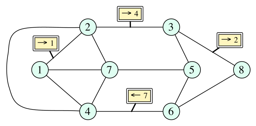
Figure 1: A graph with $4$ monitors.

Our results.

We first show that the FlowMntrs problem is NP-hard. Next, we study polynomial-time approximation algorithms. We introduce an algorithm called $\sigma$-Greedy that, in each step, places up to $\sigma$ monitors in such a way that the number of edges with known flow is maximized. We then prove that 1-Greedy is a $3$-approximation algorithm and that 2-Greedy is a $2$-approximation algorithm. The running times of these two algorithms are $O((m+n)^{2})$ and $O((m+n)^{3})$, respectively, where $n=|V|$ and $m=|E|$. In both cases, our analysis is tight. In fact, our approximation results are stronger, as they apply to the weighted case, where the input graph has weights on edges, and the objective is to maximize the total weight of the edges with known flow.

Related work.

A closely related problem was studied by Gu and Jia [4] who considered a traffic flow network with directed edges. They observed that $m-n+1$ monitors are necessary to determine the flow on all edges of a strongly connected graph, and that this bound can be achieved by placing flow monitors on edges in the complement of a spanning tree. (The same bound applies to connected undirected graphs.) Khuller et al. [5] studied an optimization problem where pressure meters may be placed on nodes of a flow network. An edge whose both endpoints have a pressure meter will have the flow determined using the pressure difference, and other edges may have the flow determined via flow conservation property. The goal is to compute the minimum number of meters needed to determine the flow on every edge in the network. They showed that this problem is NP-hard and MAX-SNP-hard, and that a local-search based algorithm achieves $2$-approximation. For planar graphs, they have a polynomial-time approximation scheme. The model in [5] differs from ours in that it assumes that the flow satisfies Kirchhoff’s current and voltage laws, while we only assume the current law (that is, the flow preservation property). This distinction is reflected in different choices of “meters”: vertex meters in [5] and edge monitors in our paper. Recall that, as explained above, minimizing the number of edge monitors needed to determine the flow on all edges is trivial, providing a further justification for our choice of the objective function.

The FlowMntrs problem is also related to the classical $k$-cut and multi-way cut problems [6, 8, 1], where the goal is to find a minimum-weight set of edges that partitions the graph into $k$ connected components. One way to view our monitor problem is that we want to maximize the number of connected components obtained from removing the monitor edges and the resulting bridge edges.

2 Preliminaries

We now give formal definitions. Let $G=(V,E)$ be an undirected graph. Throughout the paper, we use $n=|V|$ to denote the number of vertices in $G$ and $m=|E|$ to be the number of edges. We will typically use letters $u,v,x,y,...$, possibly with indices, to denote vertices, and $a,b,e,f,...$ to denote edges. If an edge $e$ has endpoints $x,y$, we write $e={\left\{x,y\right\}}$. We allow multiple edges and loops in $G$, so the endpoints do not uniquely define an edge: if $e={\left\{x,y\right\}}$ and $f={\left\{x,y\right\}}$, it is not necessarily true that $e=f$.

A circulation on $G$ is a function $\psi$ that assigns a flow value and a direction to any edge in $E$. (We use the terms “circulation” and “flow” interchangeably, slightly abusing the terminology.) Denoting by $\psi(u,v)$ the flow on $e={\left\{u,v\right\}}$ from $u$ to $v$, we require that $\psi$ satisfies the following two conditions (i) $\psi$ is anti-symmetric, that is $\psi(u,v)=-\psi(v,u)$ for each edge ${\left\{u,v\right\}}$, and (ii) $\psi$ satisfies the flow conservation property, that is $\sum_{{\left\{u,v\right\}}\in E}\psi(u,v)=0$ for each vertex $v$.

A bridge in $G$ is an edge whose removal increases the number of connected components of $G$. Let ${\mbox{\it Br}}(G)$ be the set of bridges in $G$.

Suppose that some circulation $\psi$ is given for all edges in some set $M\subseteq E$, and not for other edges. We have the following observation:

Observation 1.

For ${\left\{u,v\right\}}\in E-M$, $\psi(u,v)$ is uniquely determined from the flow preservation property if and only if ${\left\{u,v\right\}}\in{\mbox{\it Br}}(G-M)$.

We can now define the gain of $M$ to be $\mbox{\it gain}(G,M)=|M\cup{\mbox{\it Br}}(G-M)|$, that is, the total number of edges for which the flow can be determined if we place monitors on the edges in $M$. We will refer to the edges in $M$ as monitor edges, while the bridge edges in ${\mbox{\it Br}}(G-M)$ will be called extra edges. If $G$ is understood from context, we will write simply $\mbox{\it gain}(M)$ instead of $\mbox{\it gain}(G,M)$.

The Flow Edge-Monitor Problem (FlowMntrs) can now be defined formally as follows: given a graph $G=(V,E)$ and an integer $k>0$, find a set $M\subseteq E$ with $|M|\leq k$ that maximizes $\mbox{\it gain}(G,M)$.

The weighted case.

We consider the extension of FlowMntrs to weighted graphs, where each edge $e$ has a non-negative weight $w(e)$ assigned to it, and the task is to maximize the weighted gain. More precisely, if $M$ are the monitor edges, then the formula for the (weighted) gain is $\mbox{\it gain}(M)=\sum_{e\in M\cup B}w(e)$, for $B={\mbox{\it Br}}(G-M)$. We will denote this problem by WFlowMntrs.

Throughout the paper, we denote by $M^{\ast}$ some arbitrary, but fixed, optimal monitor edge set. Let $B^{\ast}={\mbox{\it Br}}(G-M^{\ast})$ be the set of extra edges corresponding to $M^{\ast}$. Then the optimal gain is ${\mbox{\it gain}^{\ast}}(G,k)=w(M^{\ast}\cup B^{\ast})$.

Simplifying assumptions.

We make some assumptions about the input graph $G$ that will simplify the proofs. First, if $k\geq m$, then we can simply take $M=E$ and this will be an optimal solution to WFlowMntrs. Therefore, without loss of generality, throughout the paper we will assume that $m>k$.

The flow value on any bridge of $G$ must be $0$, so we can assume that $G$ does not have any bridges. Further, if $G$ is not connected, we can do this: take any two vertices $u$, $v$ from different connected components and contract them into one vertex. This operation does not affect the solution to WFlowMntrs. By repeating it enough many times, we can transform $G$ into a connected graph. Summarizing, we conclude that, without loss of generality, we can assume that $G$ is connected and does not have any bridges. In other words, $G$ is $2$-edge-connected. (Recall that, for an integer $c\geq 1$, a graph $H$ is called $c$-edge-connected, if $H$ is connected and it remains connected after removing any set of at most $c-1$ edges from $H$.)

Next, we claim that can in fact restrict our attention to $3$-edge-connected graphs. To justify it, we show that any weighted 2-edge-connected graph $G=(V,E)$ can be converted in linear time into a 3-edge-connected weighted graph $G^{\prime}=(V^{\prime},E^{\prime})$ such that:

(i) ${\mbox{\it gain}^{\ast}}(G,k)={\mbox{\it gain}^{\ast}}(G^{\prime},k)$, and

(ii) If $M^{\prime}\subseteq E^{\prime}$ is a set of $k$ monitor edges in $G^{\prime}$, then in linear time one can find a set $M\subseteq E$ of $k$ monitor edges in $G$ with $\mbox{\it gain}(G,M)=\mbox{\it gain}(G^{\prime},M^{\prime})$.

We now show the construction of $G^{\prime}$. A $2$-cut is a pair of edges ${\left\{e,e^{\prime}\right\}}$ whose removal disconnects $G$. Write $e\simeq e^{\prime}$ if ${\left\{e,e^{\prime}\right\}}$ is a $2$-cut. It is known, and quite easy to show, that relation “$\simeq$” is an equivalence relation on $E$. The equivalence classes of $\simeq$ are called edge groups.

Suppose that $G$ has an edge group $F$ with $|F|=q$, for $q\geq 2$, and let $H_{1},...,H_{q}$ be the connected components of $G-F$. Then $F={\left\{e_{1},...,e_{q}\right\}}$, where, for each $i$, $e_{i}={\left\{u_{i},v_{i}\right\}}$, $u_{i}\in H_{i}$ and $v_{i}\in H_{i+1}$ (for $i=q$ we assume $q+1\equiv 1$). For $i=1,...,q-1$, contract edge $e_{i}$ so that vertices $u_{i}$ and $v_{i}$ become one vertex, and then assign to edge $e_{q}={\left\{u_{q},v_{q}\right\}}$ weight $\sum_{i=1}^{q}w(e_{i})$. We will refer to $e_{q}$ as the deputy edge for $F$. Figure 2 illustrates the construction.

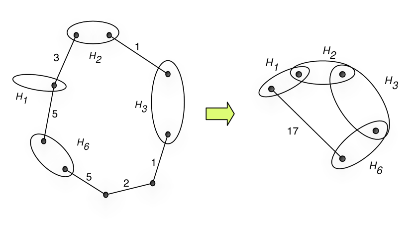
Figure 2: Contracting edge groups.

Let $G^{\prime}=(V^{\prime},E^{\prime})$ be the resulting weighted graph. By the construction, $G^{\prime}$ is $3$-edge-connected. All edge groups can be computed in linear time (see, [7], for example), so the whole transformation can be done in linear time as well.

It remains to show that $G^{\prime}$ satisfies conditions (i) and (ii). If $M$ is any monitor set, and if $M$ has two or more monitors in the same edge group, we can remove one of these monitors without decreasing the gain of $M$. Further, for any monitor edge $e$ of $M$, we can replace $e$ by the deputy edge of the edge group containing $e$, without changing the gain. This implies that, without loss of generality, we can assume that the optimal monitor set $M^{\ast}$ in $G$ consists only of deputy edges. These edges remain in $G^{\prime}$ and the gain of $M^{\ast}$ in $G^{\prime}$ will be exactly the same as its gain in $G$. This shows the “$\geq$” inequality in (i). The “$\leq$” inequality follows from the fact that any monitor set in $G^{\prime}$ consists only of deputy edges from $G$. The same argument implies (ii) as well.

Summarizing, we have shown in this section that, without loss of generality, we can assume that the input graph $G$ has $m>k$ edges and is $3$-edge-connected.

The kernel graph.

Consider an input graph $G=(V,E)$ and a monitor edge set $M$, and let $B={\mbox{\it Br}}(G-M)$. The kernel graph associated with $G$ and $M$ is defined as the weighted graph $G_{M}=(V_{M},E_{M})$, where $V_{M}$ is the set of connected components of $G-M-B$, and $E_{M}$ is determined as follows: For any edge $e\in M\cup B$, where $e={\left\{u,v\right\}}$, let $u^{\prime}$ and $v^{\prime}$ be the connected components of $G-M-B$ that contain, respectively, $u$ and $v$. Then we add edge ${\left\{u^{\prime},v^{\prime}\right\}}$ to $E_{M}$. The weights are preserved, that is $w({\left\{u^{\prime},v^{\prime}\right\}})=w({\left\{u,v\right\}})$. We will say that this edge ${\left\{u^{\prime},v^{\prime}\right\}}$ represents ${\left\{u,v\right\}}$ or corresponds to ${\left\{u,v\right\}}$. In fact, we will often identify ${\left\{u,v\right\}}$ with ${\left\{u^{\prime},v^{\prime}\right\}}$, treating them as the same object. We point out that in general $G_{M}$ is a multigraph, as it may have multiple edges and loops (even when $G$ does not). However, since $G$ is $3$-edge-connected, it is easy to see that so is $G_{M}$.

Figure 3 shows the kernel graph corresponding to the graph and the monitor set in the example from Figure 1 (all edge weights are $1$):

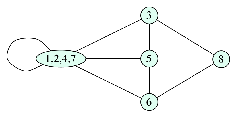
Figure 3: The kernel graph for the example in Figure 1. The loop in vertex ${\left\{1,2,4,7\right\}}$ represents edge ${\left\{2,1\right\}}$.

Note that we have $|E_{M}|\leq k+|V_{M}|-1$. This can be derived directly from the definitions: The edges in $G_{M}$ that represent extra edges are the bridges in $G_{M}$ and therefore they form a forest in $G_{M}$. This (and the fact that $G_{M}$ is connected) implies that the number of extra edges is at most $|V_{M}|-1$, and the inequality follows.

In the paper, we will use the concept of kernel graphs only with respect to some optimal monitor set. Let $M^{\ast}$ be some arbitrary, but fixed, optimal monitor edge set. To simplify notation, we will write $G^{\ast}=(V^{\ast},E^{\ast})$ for the kernel graph associated with $M^{\ast}$, that is $G^{\ast}=G_{M^{\ast}}$, $V^{\ast}=V_{M^{\ast}}$ and $E^{\ast}=E_{M^{\ast}}$. In this notation, we have ${\mbox{\it gain}^{\ast}}(G,k)=w(E^{\ast})$. In the analysis of our algorithms, we will be comparing the weights of edges collected by the algorithm against the edges in the kernel graph $G^{\ast}$.

3 Proof of NP-hardness of FlowMntrs

We show that the FlowMntrs is NP-hard (even in the unweighted case), via a reduction from the Clique problem. We start with a simple lemma.

Lemma 2.

Let $a_{1},a_{2},\ldots,a_{s}$ be $s$ positive integers such that $\sum_{i=1}^{s}a_{i}=n$, for a fixed integer $n$. Then $\sum_{i=1}^{s}\binom{a_{i}}{2}$ is maximized if and only if $a_{j}=n-s+1$ for some $j$ and $a_{i}=1$ for all $i\neq j$.

Above, we assume that $\binom{1}{2}=1(1-0)/2=0$.

Proof.

By routine algebra, one can verify that for $2\leq a\leq b$ we have

$$\binom{a}{2}+\binom{b}{2} < \binom{a-1}{2}+\binom{b+1}{2}.$$ (1)

Without loss of generality, assume $a_{1}=\max_{i}a_{i}$. If $a_{i}>1$, for any $i>1$, by the inequality above, we can change $a_{1}{\,\leftarrow\,}a_{1}+1$ and $a_{i}{\,\leftarrow\,}a_{i}-1$, increasing the value of $\sum_{i=1}^{s}\binom{a_{i}}{2}$. By repeating this argument, we obtain that an optimum is achieved for $a_{1}=n-s+1$ and $a_{2}=a_{3}=...=a_{s}=1$. That all optima have this form (up to a permutation of the $a_{i}$’s) follows from the fact that inequality (1) is strict. ∎

Theorem 3.

FlowMntrs is NP-hard.

Proof.

In the Clique problem, given an undirected graph $G=(V,E)$ and an integer $q>0$, we wish to determine if $G$ has a clique of size at least $q$. Clique is well-known to be NP-complete (see [2]). We show how to reduce Clique, in polynomial-time, to DecFlowMntrs, the decision version of FlowMntrs, defined as follows: Given a graph $G=(V,E)$ and two integers, $k,l>0$, is there a set $M$ of $k$ edges in $G$ for which $|{\mbox{\it Br}}(G-M)|\geq l$?

The reduction is simple. Suppose we have an instance $G=(V,E),q$ of Clique. Without loss of generality, we can assume that $G$ is connected and $q\geq 3$. Let $n=|V|$ and $m=|E|$. We map this instance into an instance $G,k,l$ of DecFlowMntrs, where $k=m-\binom{q}{2}-l$ and $l=n-q$. This clearly takes polynomial time. Thus, to complete the proof, it is sufficient to prove the following claim:

$(\ast)$ $G$ has a clique of size $q$ iff $G$ has a set $M$ of $k$ edges for which $|{\mbox{\it Br}}(G-M)|\geq l$.

We now prove $(\ast)$. The main idea is that, by the choice of parameters $k$ and $l$, the monitors and extra edges in the solution of the instance of DecFlowMntrs must be exactly the edges outside the size-$q$ clique of $G$.

$(\Rightarrow)$ Suppose that $G$ has a clique $C$ of size $q$. Let $G^{\prime}$ be the graph obtained by contracting $C$ into a single vertex and let $T$ be a spanning tree of $G^{\prime}$. We then take $M$ to be the set of edges of $G^{\prime}$ outside $T$. Thus the edges in $T$ will be the bridges of $G-M$. Since $G^{\prime}$ has $n-q+1$ vertices, $T$ has $l=n-q$ edges, and $M$ has $m-\binom{q}{2}-l=k$ edges.

$(\Leftarrow)$ Suppose there is a set $M$ of $k$ monitor edges that yields a set $B$ of $l^{\prime}$ extra edges, where $l\leq l^{\prime}\leq n-1$. We show that $G$ has a clique of size $q$.

Let $s$ be the number of connected components of $G-M-B$, and denote by $a_{1},a_{2},...,a_{s}$ the cardinalities of these components (numbers of vertices). Since $|B|=l^{\prime}$, we have $s\geq l^{\prime}+1$. Also, $\sum_{i=1}^{s}a_{i}=n$ and $\sum_{i=1}^{s}\binom{a_{i}}{2}+k+l^{\prime}\geq m$. Therefore, using Lemma 2, and the choice of $k$ and $l$, we have

$$\binom{n-l^{\prime}}{2}+l^{\prime} \geq \binom{n-s+1}{2}+l^{\prime}$$ (2)

$$\geq \sum_{i=1}^{s}\binom{a_{i}}{2}+l^{\prime}$$ (3)

$$\geq m-k$$

$$= \binom{n-l}{2}+l.$$

By routine calculus, the function $f(x)={\mbox{$\frac{1}{2}$}}(n-x)(n-x-1)+x$ is decreasing in interval $[0,n-1]$, and therefore the above derivation implies that $l^{\prime}\leq l$, so we can conclude that $l^{\prime}=l$. This, in turn, implies that all inequalities in this derivation are in fact equalities. Since (2) is an equality, we have $s-1=l^{\prime}=l=n-q$. Then, since (3) is an equality, Lemma 2 implies that $a_{j}=q$ for some $j$ and $a_{i}=1$ for all $i\neq j$. Finally, (3) can be an equality only if all the connected components are cliques. In particular, we obtain that the $j$th component is a clique of size $q$. ∎

4 Algorithm $\sigma$-Greedy

Fix some integer constant $\sigma\geq 1$. Let $G=(V,E)$ be the input graph with $n=|V|$, $m=|E|$, and with weights on edges. As justified in Section 2, we will assume that $m>k$ and that $G$ is $3$-edge-connected.

Algorithm $\sigma$-Greedy that we study in this section works in ${\lceil k/\sigma\rceil}$ steps and returns a set of $k$ monitor edges. In each step, it assigns $\sigma$ monitors to a set $P$ of $\sigma$ edges that maximizes the gain in this step, that is, the total weight of the monitor edges in $P$ and the bridges in $G-P$. These edges are then removed from $G$, and the process is repeated. A more rigorous description is given in Figure 4, which also deals with special cases when the number of monitors or edges left in the graph is less than $\sigma$.

Algorithm $\it\sigma$-Greedy
$\it G_{0}=(V,E_{0}){\,\leftarrow\,}G=(V,E)$
$\it M_{0}{\,\leftarrow\,}\emptyset$
$\it X_{0}{\,\leftarrow\,}\emptyset$
for $\it t{\,\leftarrow\,}1,2,...,{\lceil k/\sigma\rceil}$
if $\it E_{t-1}=\emptyset$
then return $\it M=M_{t-1}$ and halt
$\it\sigma^{\prime}{\,\leftarrow\,}\sigma$
if $\it t={\lfloor k/\sigma\rfloor}+1$
then $\it\sigma^{\prime}={k\bmod\sigma}$
if $\it|E_{t-1}|\leq\sigma^{\prime}$
then $\it P{\,\leftarrow\,}E_{t-1}$
else
find $\it P\subseteq E_{t-1}$ with $\it|P|=\sigma^{\prime}$
that maximizes $\it w(P\cup{\mbox{\it Br}}(G_{t-1}-P))$
$\it Y_{t}{\,\leftarrow\,}P\cup{\mbox{\it Br}}(G_{t-1}-P)$
$\it X_{t}{\,\leftarrow\,}X_{t-1}\cup Y_{t}$
$\it E_{t}{\,\leftarrow\,}E_{t-1}-Y_{t}$
$\it G_{t}{\,\leftarrow\,}(V,E_{t})$
$\it M_{t}{\,\leftarrow\,}M_{t-1}\cup P$
return $\it M=M_{{\lceil k/\sigma\rceil}}$

Figure 4: Pseudo-code for Algorithm $\sigma$-Greedy. $Y_{t}$ represents the edges collected by the algorithm in step $t$, with $P\subseteq Y_{t}$ being the set of monitor edges and $Y_{t}-P$ the set of extra edges. $M_{t}$ represents all monitor edges collected up to step $t$ and $X_{t}$ represents all edges collected up to step $t$.

Note that each step of the algorithm runs in time $O(m^{\sigma}(n+m))$, by trying all possible combinations of $\sigma$ edges in the remaining graph $G_{t-1}$ to find $P$. Hence, for each fixed $\sigma$, Algorithm $\sigma$-Greedy runs in polynomial time.

4.1 Analysis of 1-Greedy

In this section we consider the case $\sigma=1$. Algorithm 1-Greedy at each step chooses an edge whose removal maximizes the gain and places a monitor on this edge. This edge and its corresponding bridges are removed from the graph. This process is repeated $k$ times. We show that this algorithm has approximation ratio $3$.

Analysis.

Fix the value of $k$, and some optimal solution $M^{\ast}$ of $k$ monitor edges, and let ${G^{\ast}}=({V^{\ast}},{E^{\ast}})$ be the corresponding kernel graph. To avoid clutter, we will identify each edge in ${E^{\ast}}$ with its corresponding edge in $E$, thus thinking of ${E^{\ast}}$ as a subset of $E$. For example, when we say that the algorithm collected some $e\in{E^{\ast}}$, we mean that it collected the edge in $E$ represented by $e$.

Recall that ${\mbox{\it gain}^{\ast}}(G,k)=w({E^{\ast}})$, where $w({E^{\ast}})$ is the sum of weights of the edges in ${E^{\ast}}$. Thus we need to show that 1-Greedy’s gain is at least ${\mbox{$\frac{1}{3}$}}w({E^{\ast}})$.

Let $e_{i}$, $i=1,2,...,k$, be the $k$ heaviest edges in ${E^{\ast}}$, ordered by weight, that is $w(e_{1})\geq w(e_{2})\geq...\geq w(e_{k})$. First, we claim that for each $t=0,1,...,k$, we have

$$w(X_{t}) \geq {\textstyle\sum_{i=1}^{t}w(e_{i})},$$ (5)

where $X_{t}$ denotes the set of edges collected by the algorithm in the first $t$ steps.

The proof of (5) is by a straightforward induction. It is vacuously true for $t=0$. Suppose (5) holds for $t^{\prime}=t-1$; we will then show that it also holds for $t$. If $X_{t}$ contains all edges $e_{1},...,e_{t}$, then (5) holds. Otherwise, choose any $j$, $1\leq j\leq t$, for which $e_{j}\notin X_{t}$. By induction, $w(X_{t-1})\geq\sum_{i=1}^{t-1}w(e_{i})$, and $e_{j}$ is available to 1-Greedy in step $t$, so its gain in step $t$ is at least $w(e_{j})$. Therefore $w(X_{t})\geq w(X_{t-1})+w(e_{j})\geq w(X_{t-1})+w(e_{t})\geq\sum_{i=1}^{t}w(e_{i})$, completing the proof of (5).

Since $G$ is $3$-edge-connected, each vertex in ${G^{\ast}}$ has degree at least $3$, so $|{E^{\ast}}|\geq\frac{3}{2}|{V^{\ast}}|$, which implies that $k\geq|{E^{\ast}}|-|{V^{\ast}}|+1>{\mbox{$\frac{1}{3}$}}|{E^{\ast}}|$. Thus, from (5), we obtain that the gain of 1-Greedy is $w(X_{k})\geq\sum_{i=1}^{k}w(e_{i})\geq{\mbox{$\frac{1}{3}$}}w({E^{\ast}})$. Summarizing, we obtain:

Theorem 4.

Algorithm 1-Greedy is a polynomial-time $3$-approximation algorithm for the Weighted Flow Edge-Monitor Problem, WFlowMntrs.

With a somewhat more careful analysis, one can show that the approximation ratio of 1-Greedy is actually $3(1-1/k)$, which matches our lower bound example below.

A tight-bound example.

We now present an example showing that our analysis of 1-Greedy is tight. Graph $G$ consists of one connected component with $2k-2$ vertices, in which each vertex has degree $3$ and each edge has weight $1$, and the other connected component that has only two vertices connected by $k+2$ edges each of weight $1+\epsilon$. Fig. 5 shows the construction for $k=5$.

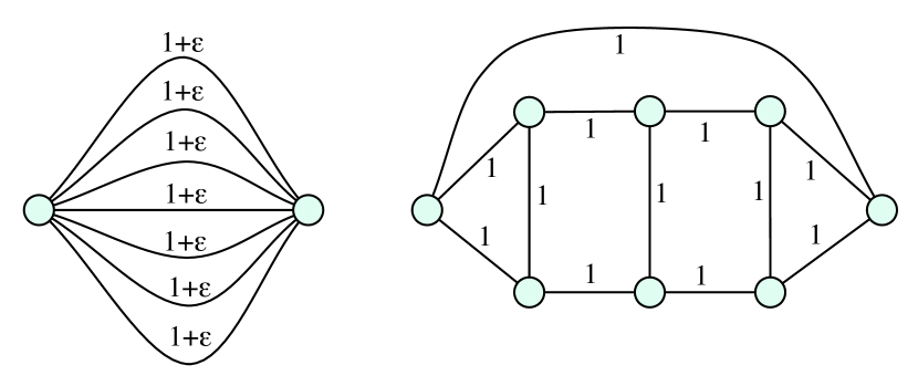
Figure 5: Lower bound example for 1-Greedy, with $k=5$.

1-Greedy will be collecting edges from the $2$-vertex component on the left, ending up with $k$ edges and total gain $(1+\epsilon)k$. The optimum solution is to put $k$ monitors in the cubic component on the right, thus gaining all $3k-3$ edges from this component. For $\epsilon\to 0$, the approximation ratio tends to $3(1-1/k)$.

4.2 Analysis of 2-Greedy

We now consider $\sigma=2$. At each step, Algorithm 2-Greedy selects two edges that maximize the gain. Ties are broken arbitrarily. We place monitors on these two edges, and then remove them from $G$, as well as the resulting bridges. The process continues for ${\lfloor{\mbox{$\frac{1}{2}$}}k\rfloor}$ steps. Exceptional situations, when $k$ is odd, or we run out of edges, etc., are handled as in Figure 4. In this section we show that 2-Greedy is a $2$-approximation algorithm.

Idea of the analysis.

Let $G=(V,E)$ be the input graph with weights on edges. As before, we will assume that $m>k$ and that $G$ is $3$-edge-connected. We can further assume that 2-Greedy never runs out of edges, for otherwise it computes an optimal solution. We fix some optimal solution $M^{\ast}$, and let ${G^{\ast}}=({V^{\ast}},{E^{\ast}})$ be the corresponding kernel graph with $\nu=|{V^{\ast}}|$ vertices and $\mu=|{E^{\ast}}|$ edges. Recall that ${\mbox{\it gain}^{\ast}}(G,k)=w({E^{\ast}})$; thus we need to show that 2-Greedy’s gain is at least ${\mbox{$\frac{1}{2}$}}w({E^{\ast}})$.

Our proof for 1-Greedy was based on the observation that $k\geq{\mbox{$\frac{1}{3}$}}|{E^{\ast}}|$; thus we only needed to show that 1-Greedy’s gain is at least the total weight of the $k$ heaviest edges in ${E^{\ast}}$. This is not sufficient for 2-Greedy. To see this, consider a simple situation where $G^{\ast}$ is unweighted with all vertices of degree $3$, the extra edges form a tree in ${G^{\ast}}$, and $k$ is even. Then $\mu={\mbox{$\frac{3}{2}$}}\nu$ and $\mu=\nu+k-1$, so $\mu\approx 3k$. Therefore we need to show that in this case 2-Greedy collects at least ${\mbox{$\frac{3}{2}$}}k$ edges. For the unweighted graph, this is not hard to show: pick a set $J$ of ${\mbox{$\frac{1}{2}$}}k$ independent vertices in ${G^{\ast}}$. For each vertex $v$ in $J$, at each step of 2-Greedy, either the three edges of $v$ have already been collected, or they can be collected in this step by placing monitors on two of them. (It is also possible that one edge out of $v$ has already been collected, but in this case the remaining two can be collected in this step as well.) Therefore the gain of 2-Greedy in ${\mbox{$\frac{1}{2}$}}k$ steps will be at least the number of edges out of $J$, that is ${\mbox{$\frac{3}{2}$}}k$.

If $G$ is weighted, the argument above is not sufficient, since the edges incident to vertices in $J$ may have small weights. Further, it may happen that 2-Greedy will collect only $k$ edges in total, if they are heavy enough, and in this case we need to argue that their total weight is at least ${\mbox{$\frac{1}{2}$}}w({E^{\ast}})$, even though $k$ may be only about ${\mbox{$\frac{1}{3}$}}|{E^{\ast}}|$.

The proof consists of two parts. First, we introduce the concept of a bundle. Intuitively, a bundle is a set of edges that can be collected with at most two monitors, although our definition is more restrictive and will be given shortly. We show that ${G^{\ast}}$ contains a set $T$ of at most ${\lfloor{\mbox{$\frac{1}{2}$}}k\rfloor}$ disjoint bundles with total weight at least ${\mbox{$\frac{1}{2}$}}w({E^{\ast}})$. In the second part of the proof we show that the gain of 2-Greedy is at least the total weight of $T$.

Analysis.

For any vertex in ${G^{\ast}}$ of degree $3$, the set of three edges incident on this vertex is called a tripod. A set $\beta$ of edges is called a bundle if $\beta$ is either a tripod or it consists of at most two edges. Clearly, all edges of a bundle can be collected with at most $2$ monitors. If $T$ is a set of bundles, by $E_{T}$ we denote the set of edges in $T$, that is $E_{T}=\bigcup_{\beta\in T}\beta$. (We will extend the definition of bundles later in the proof of Lemma 6.)

Lemma 5.

For $k\geq 2$, there exists a set $T$ of at most ${\lfloor k/2\rfloor}$ disjoint bundles such that $w(E_{T})\geq{\mbox{$\frac{1}{2}$}}w({E^{\ast}})$.

Proof.

First, we construct a collection $Z$ of bundles that contains all tripods in ${G^{\ast}}$ and such that each edge appears in exactly two bundles in $Z$. To this end, we create two copies of each edge. If $e={\left\{x,y\right\}}$ is an edge, then by $e^{x}$ and $e^{y}$ we will denote these two copies of $e$. Let $F$ be the set of all these edge copies.

For each vertex $v$ of ${G^{\ast}}$ of degree $3$, if $e$, $f$, $g$ are the edges incident to $v$, add the tripod $\beta={\left\{e^{v},f^{v},g^{v}\right\}}$ to $Z$ and remove $e^{v}$, $f^{v}$ and $g^{v}$ from $F$. Let $F^{\prime}$ be the set of remaining edges in $F$.

We now want to partition $F^{\prime}$ into pairs, with each pair becoming a bundle. Assume first that $|F^{\prime}|$ is even; the argument for the general case is essentially the same but slightly more cumbersome because of the parity issue, and it will be explained later.

Group the edges in $F^{\prime}$ arbitrarily into pairs. As long as any of these pairs has two copies of the same edge, say ${\left\{e^{x},e^{y}\right\}}$, do this: take any other pair ${\left\{f^{u},g^{v}\right\}}$ (where possibly $f=g$) and replace these two pairs by pairs ${\left\{e^{x},f^{u}\right\}}$ and ${\left\{e^{y},g^{v}\right\}}$. Eventually each pair will contain different edges. All these pairs become bundles that are now added to $Z$. This completes the construction of $Z$.

To construct $T$, we now greedily extract from $Z$ non-overlapping bundles with maximum weight. More specifically, we start with $T=\emptyset$, and repeat the following step as long as $|Z|\geq 4$: choose a bundle $\beta$ in $Z$ with maximum $w(\beta)$, add it to $T$, and then remove from $Z$ exactly four bundles: $\beta$, all other bundles in $Z$ that intersect $\beta$, and possible a few more additional bundles so that the total is four. This is possible, because, by the definition of $Z$, each bundle in $Z$ intersects at most three other bundles in $Z$. If, at the end, $|Z|\neq\emptyset$, then we add to $T$ the bundle $\beta$ in $Z$ with maximum $w(\beta)$ and remove all remaining bundles (at most three) from $Z$.

We now have our set $T$ of bundles, and it remains to show that it has the desired properties. Obviously, all bundles in $T$ are disjoint. In each step of the construction of $T$, when we add a bundle $\beta$ to $T$, we reduce $w(E_{Z})$ by at most $4w(\beta)$, so $w(E_{T})\geq{\mbox{$\frac{1}{4}$}}w(E_{Z})={\mbox{$\frac{1}{2}$}}w({E^{\ast}})$, as needed.

It remains to show that $|T|\leq{\lfloor{\mbox{$\frac{1}{2}$}}k\rfloor}$. Let $\nu_{d}$ be the number of vertices of degree $d$ in ${G^{\ast}}$. All vertices in ${G^{\ast}}$ have degree at least $3$, thus

$$2\mu\;=\;{\textstyle\sum_{d\geq 3}d\cdot\nu_{d}}\;\geq\;3\nu_{3}+4(\nu-\nu_{3})\;=\;4\nu-\nu_{3}.$$

We also have $\mu\leq\nu+k-1$, which, together with the inequality above yields $2\mu-\nu_{3}\leq 4k-4$. In $Z$, we have exactly $\nu_{3}$ tripods and ${\mbox{$\frac{1}{2}$}}(2\mu-3\nu_{3})=\mu-{\mbox{$\frac{3}{2}$}}\nu_{3}$ pairs, so we obtain $|Z|=\mu-{\mbox{$\frac{1}{2}$}}\nu_{3}\leq 2k-2$. Hence $|T|\leq{\lceil(2k-2)/4\rceil}={\lceil(k-1)/2\rceil}\leq{\lfloor{\mbox{$\frac{1}{2}$}}k\rfloor}$, as needed.

Now we deal with the case when $|F^{\prime}|$ is odd. We execute the same process for pairing edges, but in this case we will end up with one unpaired edge that will become a bundle by itself. The proof that $w(E_{T})\geq{\mbox{$\frac{1}{2}$}}w({E^{\ast}})$ remains valid. We still need to show that $|T|\leq{\lfloor{\mbox{$\frac{1}{2}$}}k\rfloor}$. In $Z$, we have $\nu_{3}$ tripods, ${\mbox{$\frac{1}{2}$}}(2\mu-3\nu_{3}-1)$ pairs, and one singleton; hence $|Z|=\nu_{3}+{\mbox{$\frac{1}{2}$}}(2\mu-3\nu_{3}-1)+1={\mbox{$\frac{1}{2}$}}(2\mu-\nu_{3}+1)$. As before, we have $2\mu-\nu_{3}\leq 4k-4$, but now $2\mu-\nu_{3}=(2\mu-3\nu_{3})+2\nu_{3}=|F^{\prime}|+2\nu_{3}$ is odd, which implies that we in fact have $2\mu-\nu_{3}+1\leq 4k-4$. This implies $|Z|\leq 2k-2$, and the bound $|T|\leq{\lfloor k/2\rfloor}$ follows, as before. ∎

Lemma 6.

Let $k\geq 2$, and let $T$ be the set of bundles constructed in Lemma 5. Then $w(X_{{\lfloor k/2\rfloor}})\geq w(E_{T})$; thus 2-Greedy’s gain is at least $w(E_{T})$.

Proof.

Let $\ell={\lfloor k/2\rfloor}$. To prove the lemma, we show that there is a partition of $E_{T}$ into disjoint sets $B_{1},B_{2},...,B_{\ell}$ (some possibly empty) such that $w(B_{t})\leq w(Y_{t})$, for $t=1,2,...,\ell$, where $Y_{t}$ is the set of edges collected by 2-Greedy in step $t$. This is clearly sufficient to establish the theorem.

The idea of the proof is to proceed one step at a time, for $t=1,2,...,\ell$, starting with $T^{\prime}=T$ and at each step reducing the number of bundles in $T^{\prime}$. The invariant will be that at each step $t$, all bundles in $T^{\prime}$ will be available to 2-Greedy for collection. At step $t$, we eliminate from these bundles all edges collected by the algorithm, and rearrange some bundles, if necessary, in such a way that the number of bundles in $T^{\prime}$ strictly decreases.

To implement the above idea we need to extend the definition of bundles. If $\beta={\left\{e,f,g\right\}}$ is a tripod in ${G^{\ast}}$ and 2-Greedy collects $e$ at some step $t^{\prime}<t$ while $f,g$ remain uncollected until step $t$, then the pair $\beta^{\prime}={\left\{f,g\right\}}$ is called a bipod at step $t$. If $\beta\subseteq{E^{\ast}}$ is a set of edges not collected in the first $t-1$ steps, then $\beta$ is called a bundle at step $t$ if either (i) $\beta$ is a tripod in ${G^{\ast}}$, or (ii) $\beta=\beta_{1}\cup\beta_{2}$, where each $\beta_{i}$ is either an edge or a bipod or $\emptyset$. (We will omit phrase “at time $t$” whenever $t$ is understood from context.) Clearly, this definition extends the one given earlier in this section. However, it is still true that 2-Greedy can collect all edges from a bundle in a single step (that is, with two monitors).

Now we describe the construction of the sets $B_{t}$. Initially, $T^{\prime}=T$. Suppose that, for some $t\geq 1$, we have already constructed $B_{1},...,B_{t-1}$ and modified $T^{\prime}$ accordingly. Consider now step $t$ of 2-Greedy. We distinguish three cases.

Case 1: $Y_{t}$ intersects at most one bundle in $T^{\prime}$. If $Y_{t}$ intersects one bundle, let $\beta$ be this bundle; otherwise, let $\beta$ be any bundle. Remove $\beta$ from $T$ and set $B_{t}=\beta$.

Case 2: $Y_{t}$ contains a bundle in $T^{\prime}$. In this case we simply set $B_{t}=Y_{t}\cap E_{T^{\prime}}$ and we update $T^{\prime}$ as follows: remove from $T^{\prime}$ all bundles that are contained in $Y_{t}$, and for each other bundle $\beta$ in $T^{\prime}$ that intersects $Y_{t}$, remove from $\beta$ the edges in $Y_{t}$ (that is, $\beta{\,\leftarrow\,}\beta-Y_{t}$).

Case 3: $Y_{t}$ intersects at least two bundles in $T^{\prime}$ but it does not contain any. We let $B_{t}=Y_{t}\cap E_{T^{\prime}}$. To update $T^{\prime}$, we proceed in two steps. First, choose any two bundles $\beta_{1},\beta_{2}$ in $T^{\prime}$ intersected by $Y_{t}$, and replace them by $\beta_{1}\cup\beta_{2}-Y_{t}$. Then, for each other bundle $\beta$ in $T^{\prime}$ intersected by $Y_{t}$, remove from $\beta$ all edges in $Y_{t}$.

Note that Cases 2 and 3 are not mutually exclusive. If, at some steps, both of these cases apply, any of them can be chosen arbitrarily.

We claim that this procedure is correct, in the sense that at each step $t$ all elements of $T^{\prime}$ are bundles. To this end, we make two observations. If $\beta={\left\{e,f,g\right\}}$ is a tripod at time $t$, then 2-Greedy can either collect one edge from $\beta$ or all three, but it cannot collect just two. If one edge is collected, the remaining edges form a bipod. Also, if ${\left\{e,f\right\}}$ is a bipod at time $t$, then 2-Greedy either collects both edges $e,f$ or none. If we remove any edges from a bundle, it obviously remains a bundle. Another type of update occurs in Case 3 where we replace $\beta_{1}$ and $\beta_{2}$ by $\beta_{1}\cup\beta_{2}-Y_{t}$. Here, by the case condition, each $\beta_{i}-Y_{t}$ is either an edge or a bipod, and thus $\beta_{1}\cup\beta_{2}-Y_{t}$ is a correct bundle.

Next, we estimate the weight of the sets $B_{t}$. In Cases 2 and 3 we have $B_{t}\subseteq Y_{t}$, so clearly $w(Y_{t})\geq w(B_{t})$. Due to the fact that it takes no more than two monitors to collect all edges in a bundle and 2-Greedy chooses $Y_{t}$, $w(Y_{t})$ is at least as large as the weight of any bundle in $T^{\prime}$ at time $t$; hence $w(Y_{t})\geq w(B_{t})$ holds for Case 1 as well.

Finally, note that we have no more than $\ell$ bundles in $T^{\prime}$ to start with and the total number of bundles in $T^{\prime}$ strictly decreases in each step. Therefore after $\ell$ steps we will have $T^{\prime}=\emptyset$, and thus $B_{1},B_{2},...,B_{\ell}$ is a partition of $E_{T}$, completing the proof. ∎

In the case for $k=1$, 2-Greedy actually gets an optimal solution, and Lemma 5 and 6 combined imply that for $k\geq 2$ the gain of 2-Greedy is at least half of the optimum. Thus, summarizing, we obtain our main result.

Theorem 7.

Algorithm 2-Greedy is a polynomial-time $2$-approximation algorithm for the Weighted Flow Edge-Monitor Problem, WFlowMntrs.

A tight-bound example.

Our analysis of 2-Greedy is tight. The example is essentially the same as the one for 1-Greedy, illustrated in Figure 5, except that the edges in the 2-vertex component on the left side have now weights $1.5+\epsilon$. 2-Greedy will be collecting edges from this 2-vertex component, so its total gain will be $(1.5+\epsilon)k$, while the optimum gain is $3k-3$. For $\epsilon\to 0$ and $k\to\infty$, the ratio tends to $2$.

5 Final Comments

The most intriguing open question is what is the approximation ratio of $\sigma$-Greedy in the limit for $\sigma\to\infty$. We can show that this limit is not lower than $1.5$, and we conjecture that $1.5$ is indeed the correct answer.

A natural question to ask is whether our results can be extended to directed graphs. It is not difficult to show that this is indeed true; both the NP-hardness proof and $2$-approximation can be adapted to that case.

Another intriguing direction to pursue would be to study the extension of our problem to arbitrary linear systems of equations. In that context, we can put $k$ “monitors” on $k$ variables of the system to measure their values. The objective is to maximize the number of variables whose values can be uniquely deduced from the monitored variables.

References

- [1] Dahlhaus, E. and Johnson, D.S., and Papadimitriou, C.H. and Seymour, P.D. and Yannakakis, M.: The Complexity of Multiway Cuts (Extended Abstract). In: 24th ACM Symposium on Theory of Computing, STOC, pp. 241-251. ACM, New York (1992)
- [2] Garey, M.R. and Johnson, D.S.: Computers and Intractability: A Guide to the Theory of NP-Completeness. W. H. Freeman (1979)
- [3] Goldschmidt, O and Hochbaum, D.S: Polynomial Algorithm for the k-Cut Problem. In: 29th Annual IEEE Symposium on Foundations of Computer Science, FOCS, pp. 444-451. IEEE Computer Society, Washington, DC, USA (1988)
- [4] Gu, W. and Jia X.: On a Traffic Control Problem. In: 8th International Symposium on Parallel Architectures,Algorithms and Networks , I-SPAN, pp. 510–515, IEEE Computer Society, Washington, DC, USA (2005)
- [5] Khuller, S. Bhatia, R. and Pless, R.: On Local Search and Placement of Meters in Networks. SIAM J on Comput. 32, 470-487 (2003)
- [6] Saran, H. and Vazirani, V.V.: Finding k-cuts within Twice the Optimal. In: 32nd Annual Symposium on Foundations of Computer Science, FOCS, pp. 743-751. IEEE Computer Society, Washington, DC, USA (1991)
- [7] Tsin, Y.H.: A Simple 3-Edge-Connected Component Algorithm. Theor. Comp. Sys. 40, 125–142 (2007)
- [8] Vazirani, V.V.: Approximation Algorithms. Springer (2001)