Universal Thermoelectric Effect of Dirac Fermions in Graphene

Abstract

We numerically study the thermoelectric transports of Dirac fermions in graphene in the presence of a strong magnetic field and disorder. We find that the thermoelectric transport coefficients demonstrate universal behavior depending on the ratio between the temperature and the width of the disorder-broadened Landau levels(LLs). The transverse thermoelectric conductivity $\alpha_{xy}$ reaches a universal quantum value at the center of each LL in the high temperature regime, and it has a linear temperature dependence at low temperatures. The calculated Nernst signal has a peak at the central LL with heights of the order of $k_{B}/e$, and changes sign near other LLs, while the thermopower has an opposite behavior, in good agreement with experimental data. The validity of the generalized Mott relation between the thermoelectric and electrical transport coefficients is verified in a wide range of temperatures.

Graphene has attracted enormous interest due to its unique electronic properties associated with the two-dimensional (2D) Dirac-fermion excitations  CastroNeto09 , including its thermoelectric properties Kim09 ; Shi09 ; Ong08 . The thermopower and Nernst coefficient, measuring the magnitude of the longitudinal and transverse electric fields generated in response to an applied temperature gradient, are very sensitive to the semimetal nature of graphene. For instance, a large thermopower is expected near the Dirac point as $S_{xx}\sim T/E_{F}$ while $T$ and $E_{F}$ are the temperature and the Fermi energy, respectively. This has been observed in recent experiments  Kim09 ; Shi09 ; Ong08 , where the maximum value of thermopower reaches $90\mu V/K$ at $T\approx 300K$.

In a magnetic field, the electronic states of graphene are quantized into Landau levels (LLs), as in the 2D semiconductor systems displaying the integer quantum Hall effect (IQHE) Prange87 . However, the Hall conductivity of graphene obeys an unconventional quantization rule $\sigma_{xy}=4(n+1/2)e^{2}/h$, where $n$ is an integer Novoselov05 ; Zhang05 ; Haldane88 ; Gusynin05 . For the conventional 2D IQHE systems, theories Girvin82 ; Streda83 ; Jonson84 ; Oji84 predict that when the thermal activation dominates the broadening of LLs, all transport coefficients are universal functions of $E_{F}/\hbar\omega_{c}$ and $k_{B}T/\hbar\omega_{c}$, where $\hbar\omega_{c}$ is the LL quantization energy. $S_{xx}$ shows a series of peaks near the LL energies with height $\ln 2(k_{B}/e)/(n+1/2)$, which is independent of the magnetic field or temperature. The Nernst signal $S_{xy}$ oscillates about zero near the LLs and enhances as the strength of the impurity scattering increases. The experimental results on graphene agree with these asymptotic behaviors except at the central LL, where $S_{xy}$ has a peak instead with maximum value about $40\mu V/K$ while $S_{xx}$ becomes oscillatory Kim09 ; Shi09 ; Ong08 . The unusual behavior of $S_{xy}$ and $S_{xx}$ near the central LL has not been understood.

While thermoelectric transports depend crucially on impurity scattering as well as thermal activation, the study of disorder effect on thermoelectric transports in graphene is still lacking. Another important question is to what extent the well-known Mott relation between thermoelectric and electrical transport coefficients [cf. Eq.(3)] is applicable for this system. In this Letter, we carry out a numerical study to address all the above issues. We show that thermoelectric transport coefficients are universal functions of the ratio between the temperature and the disorder-induced LL width, and display different asymptotic behaviors in different temperature regions, in agreement with experimental data. Our study also reveals that the distinct behaviors in the central LL is an intrisic property of the Dirac point where both particle and hole LLs coexist. Furthermore, the generalized Mott relation is shown to be valid for a wide range of temperatures.

We consider a rectangular sample of a 2D graphene sheet consisting of carbon atoms on a honeycomb lattice Sheng05 . Besides the Anderson-type random disorder considered in Ref.Sheng05 , we also model charged impurities in substrate, randomly located in a plane at a distance $d$, either above or below the graphene sheet with a long-range Coulomb scattering potential. The latter type of disorder is known Adam07 to give a more satisfactory interpretation of the transport properties of graphene in the absence of magnetic fields. When a magnetic field is applied perpendicular to the graphene plane, the Hamiltonian can be written in the tight-binding form

$$H=-t\sum\limits_{\langle ij\rangle\sigma}e^{ia_{ij}}c_{i\sigma}^{\dagger}c_{j\sigma}+\sum_{i\sigma}w_{i}c_{i\sigma}^{\dagger}c_{i\sigma},$$ (1)

where $c_{i\sigma}^{+}$ ($c_{i\sigma}$) creates (annihilates) a $\pi$ electron of spin $\sigma$ on lattice site $i$. $t$ is the nearest-neighbor hopping integral with an additional phase factor $a_{ij}$ due to the applied magnetic field $B$. The magnetic flux per hexagon $\phi=\sum_{{\small{\mbox{\hexagon}}}}a_{ij}=\frac{2\pi}{M}$ with $M$ an integer  Sheng05 . For Anderson-type disorder, $w_{i}$ is randomly distributed between $[-W/2,W/2]$ with $W$ as the disorder strength. For charged impurities, $w_{i}=-\frac{Ze^{2}}{\kappa}\sum_{\alpha}1/\sqrt{({\bf r}_{i}-{\bf R}_{\alpha})^{2}+d^{2}}$, where $Ze$ is the charge carried by the impurities, $\kappa$ is the effective background lattice dielectric constant, and ${\bf r}_{i}$ and ${\bf R}_{\alpha}$ are the planar positions of site $i$ and impurity $\alpha$, respectively. All the properties of the substrate (or vacuum in the case of suspended graphene) can be absorbed into a dimensionless parameter $r_{s}=Ze^{2}/(\kappa\hbar v_{F})$, where $v_{F}$ is the Fermi velocity of the electrons. For simplicity, in the following calculation, we fix the value of distance $d=1$, randomly distribute impurities with the density as $1\%$ of the total sites, and tune $r_{s}$ to control the impurity scattering strength.

In the linear response regime, the charge current in response to an electric field or a temperature gradient can be written as ${\bf J}={\hat{\sigma}}{\bf E}+{\hat{\alpha}}(-\nabla T)$, where ${\hat{\sigma}}$ and ${\hat{\alpha}}$ are the electrical and thermoelectric conductivity tensors, respectively. These transport coefficients can be calculated with Kubo formula once we obtain all the eigenstates of the Hamiltonian (in our calculation, $\sigma_{xx}$ is obtained based on the calculation of the Thouless number Ma08 ). In practice, we can first calculate the $T=0$ conductivities $\sigma_{ji}(E_{F})$, and then use the relation Jonson84

$$\sigma_{ji}(E_{F},T) = \int d\epsilon\,\sigma_{ji}(\epsilon)\left(-{\partial f(\epsilon)\over\partial\epsilon}\right),$$

$$\alpha_{ji}(E_{F},T) = {-1\over eT}\int d\epsilon\,\sigma_{ji}(\epsilon)(\epsilon-E_{F})\left(-{\partial f(\epsilon)\over\partial\epsilon}\right),$$ (2)

to obtain the finite temperature electrical and thermoelectric conductivity tensors. Here $f(x)=1/[e^{(x-E_{F})/k_{B}T}+1]$ is the Fermi distribution function. At low temperatures, the second equation can be approximated as

$$\alpha_{ji}(E_{F},T)=-\frac{\pi^{2}k_{B}^{2}T}{3e}\left.\frac{d\sigma_{ji}(\epsilon,T)}{d\epsilon}\right|_{\epsilon=E_{F}},$$ (3)

which is the generalized Mott relation Jonson84 ; Oji84 .

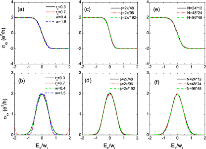
Figure 1: (color online). Zero temperature $\sigma_{xy}$ and $\sigma_{xx}$ as functions of the normalized Fermi energy near the Dirac point with $W_{L}$ as the width of the central LL. (a) and (b) compare results for short-range random potential (with various $W$) and long-range Coulomb potential (with various $r_{s}$), where the system size $N=96\times 48$ and the magnetic flux $\phi=\frac{2\pi}{48}$. (c) and (d) compare results for three different strengths of magnetic flux, with the same system size $N=96\times 48$ and the same impurity configuration, where a long-range scattering potential with $r_{s}=0.4$ is assumed. (e) and (f) are for three different system sizes with $r_{s}=0.3$ and $\phi=\frac{2\pi}{24}$.

In Fig.1, we show the calculated Hall conductivity $\sigma_{xy}$ and longitudinal conductivity $\sigma_{xx}$ at $T=0$ as functions of the Fermi energy near the Dirac point. From Fig. 1 (a) and (b), we observe that the results for the two different types of disorder are very similar. The Hall conductivity exhibits two well-quantized plateaus $-2e^{2}/h$ and $2e^{2}/h$, being consistent with the quantization rule $\sigma_{xy}=4(n+1/2)e^{2}/h$. The direct transition between the two plateaus is accompanied by a pronounced peak in the longitudinal conductivity $\sigma_{xx}$ with the maximum value $2e^{2}/h$ footnote2 . Remarkably, once we scale the energy with the width of the central LL ($W_{L}$), which is determined by the full-width at half-maximum of the $\sigma_{xx}$ peak, all results fall into a single curve, though there are small deviations for $\sigma_{xx}$ at the peak tails. This is rather in accordance with the scaling theory on the quantum Hall liquid to insulator transition Sondhi97 , as $W_{L}$ corresponds to an energy scale where the electron localization length (correlation length) is comparable to the system size. The scaling is further tested for different magnetic fields and different system sizes, as shown in Figs. 1(c-d) and Figs. 1(e-f), respectively. We conclude that, when $E_{F},W_{L}\ll\hbar\omega_{c}$, $\sigma_{xx}$ and $\sigma_{xy}$ are universal functions of a single parameter $E_{F}/W_{L}$ . It is noteworthy that the universal curves shown in Fig. 1 are for disorder strengths smaller than the critical values, which is relevant to the experiments Kim09 ; Shi09 ; Ong08 . With stronger disorder strength, an insulating state may appear at the Dirac point Sheng05 .

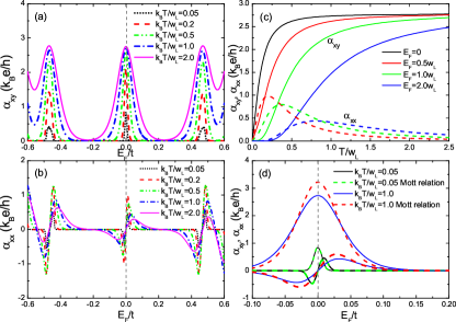
Figure 2: (color online). Thermoelectric conductivities at finite temperatures. (a) and (b) show $\alpha_{xy}(E_{F},T)$ and $\alpha_{xx}(E_{F},T)$ as functions of the Fermi energy at different temperatures. (c) shows the temperature dependence of $\alpha_{xy}(E_{F},T)$ and $\alpha_{xx}(E_{F},T)$ for certain fixed Fermi energies. (d) compares the results from numerical calculations and from the generalized Mott relation at two characteristic temperatures, $k_{B}T/W_{L}=0.05$ and $k_{B}T/W_{L}=1$. The other parameters are taken to be $N=96\times 48$, $\phi=2\pi/48$, and $r_{s}=0.3$ with $W_{L}/t=0.0195$.

In Fig. 2, we show the results of thermoelectric conductivities $\alpha_{xy}$ and $\alpha_{xx}$ at finite temperatures. As seen from Fig.2(a) and (b), $\alpha_{xy}$ displays a series of peaks near the LL energies, while ${\alpha_{xx}}$ oscillates and changes sign at the LL energies. These behaviors are similar to those in the conventional IQHE systems Jonson84 , but some important differences exist. First, at low temperatures, the peak of $\alpha_{xy}$ at the central LL is higher and narrower than at the other LLs, which indicates that the impurity scattering has a different effect on the central LL and the rest LLs. Second, $\alpha_{xy}$ and $\alpha_{xx}$ are symmetric and antisymmetric about the Dirac point (zero energy), respectively, as they are even and odd functions of the Fermi energy, rather than periodic functions. We also find that, depending on the relative strength between $k_{B}T$ and $W_{L}$, the thermoelectric conductivities show different universal behaviors. When $k_{B}T\ll W_{L}$ and $E_{F}\ll W_{L}$, we find that both $\alpha_{xy}$ and $\alpha_{xx}$ are linear in $T$ (verified by a log-log plot to the lowest temperature accessible by numerics). This indicates that within the mobility edge where extended states dominate, the diffusive transports play important roles as in semiclassical Drude-Zener regime. When the Fermi energy falls deep inside the mobility gap or $k_{B}T$ becomes comparable to or greater than $W_{L}$, thermal activation dominates. In this regime, $\alpha_{xx}$ assumes the Arrhenius form $(1/T)e^{-E_{F}/k_{B}T}$. Meanwhile, the heights of the peaks in $\alpha_{xy}$ for all LLs saturate to a value $2.77k_{B}e/h$, as seen from Fig.2(c). This value matches exactly the universal number $(\ln 2)k_{B}e/h$ predicted for the conventional IQHE systems in the case where thermal activation dominates Jonson84 ; Oji84 , with an additional degeneracy factor $4$.

To examine the validity of the generalized Mott relation, we compare the above results with those calculated from Eq.(3), as shown in Fig.2(d). The Mott relation, which was historically derived from the semiclassical Boltzmann equation, is a low-temperature approximation and predicts that thermoelectric conductivities are linear in temperature. This is in agreement with our low-temperature results. At high temperatures, thermoelectric conductivities deviate from the linear-$T$ dependence. However, if we take into account the finite temperature values of electrical conductivities, the Mott relation still predicts the correct asymptotic behavior. This is due to the fact that the conductivities display universal dependence on $E_{F}/k_{B}T$, either a power law or an exponential function in different regimes, which can all be captured by the Mott relation. This proves that the generalized Mott relation is asymptotically valid in Landau-quantized systems, as suggested in Ref. Jonson84 .

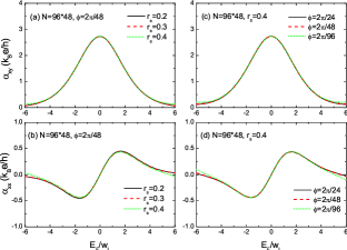
Figure 3: (color online). Universal behaviors of $\alpha_{xx}$ and $\alpha_{xy}$ near the central LL at $k_{B}T/W_{L}=1$. (a)(b) show them as functions of the renormalized Fermi energy for three disorder strengths, and (c)(d) compare results for different magnetic fields. The parameters chosen are shown in the figure.

Given the single-parameter scaling behaviors of the $T=0$ conductivities, it is straightforward to show with Eq.(2) that $\sigma_{ji}$ and $\alpha_{ji}$ at finite temperatures are universal functions of $W_{L}/k_{B}T$ and $E_{F}/k_{B}T$, or

$${\cal L}(E_{F},T)={\cal L}_{0}S_{\cal L}\left({E_{F}/W_{L}},{W_{L}/k_{B}T}\right),$$ (4)

where ${\cal L}$ stands for one of the transport coefficients and $S_{\cal L}(x,y)$ is a universal function. We can directly verify the universal relations Eq.(4). Here, we pick a temperature $k_{B}T=W_{L}$, corresponding to $S_{\cal L}(x,1)$, and compare the results around the central LL for different disorder strengths and different magnetic fields, as shown in Fig. 3. Indeed, once we scale the Fermi energy with $W_{L}$, $\alpha_{xx}$ and $\alpha_{xy}$ as functions of $E_{F}/W_{L}$ collapse into the same corresponding curves.

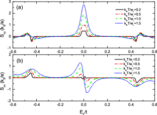
Figure 4: (color online). Calculated (a) $S_{xx}$ and (b) $S_{xy}$ as functions of the Fermi energy for different temperatures. The parameters chosen here are the same as in Fig.2.

We note that the asymptotic behaviors and the values of the peak heights of our calculated $\alpha_{xx}$ and $\alpha_{xy}$ are in agreement with the experimental results Ong08 . We further calculate the thermopower $S_{xx}$ and the Nernst signal $S_{xy}$ using Jonson84

$$S_{ij}=E_{j}/\nabla_{i}T=\sum_{k=x,y}[{\hat{\sigma}}^{-1}]_{ik}\alpha_{kj},$$ (5)

which are directly determined in experiments by measuring the responsive electric fields. The results for three central LLs are shown in Fig. 4. $S_{xy}$ ($S_{xx}$) has a peak at the central LL (the other LLs), and changes sign near the other LLs (the central LL). The height of the $S_{xx}$ peak at $n=-1$ LL is found to be $37\mu V/K$ for $k_{B}T=0.2W_{L}$ and $56\mu V/K$ for $k_{B}T=0.5W_{L}$, which is in agreement with the maximum measured value $48\mu V/K$Ong08 . This is also in agreement with the theory predication that, in the absence of disorder and at low temperatures, the peak value of $S_{xx}$ is dominated by $\alpha_{xy}/\sigma_{xy}$ and takes a universal value $(2/3)\ln 2k_{B}/e\approx 40\mu V/K$. In the presence of disorder and at finite temperatures, the peak value is slightly bigger and the peak position is shifted toward $E_{F}=0$. At $E_{F}=0$, both $\sigma_{xy}$ and $\alpha_{xx}$ vanish, leading to a vanishing $S_{xx}$. Around the zero energy, because $\sigma_{xx}\alpha_{xx}$ and $\sigma_{xy}\alpha_{xy}$ have opposite signs, depending on their relative magnitudes, $S_{xx}$ increases or decreases when the Fermi energy is increased passing the Dirac point. In our calculations, we find that the second term is always dominant, which is different from the experimental observation. This might be related to the unexpected large value of $\sigma_{xx}\sim 6e^{2}/h$ observed in experiments. Figure  4 actually shows the result when we rescale $\sigma_{xx}$ to the experimental value instead of the theoretical result $2e^{2}/h$. We can then obtain the same asymptotic behavior as in experiments for $k_{B}T=0.2W_{L}$. On the other hand, $S_{xy}$ has a peak structure, which is dominated by $\alpha_{xy}/\sigma_{xx}$. With the rescaled $\sigma_{xx}$, we find that the peak height is $40\mu V/K$ at $k_{B}T=0.2W_{L}$, which is comparable with the experimental value $20-40\mu V/K$. The distinct thermoelectric behaviors near the central LL can be traced down to the Berry phase anomaly of the Dirac point. The central LL in graphene in fact consists of two degenerate LLs, one from particles and another from holes, which are protected by the particle-hole symmetry. While this makes no distinction in electrical transports when the energy is tuned through the LL, electrons and holes contribute differently in thermoelectric transports than in electrical transports. Here, the contributions of equal numbers of electrons and holes moving along the same thermal gradient direction cancel with each other in $S_{xx}$ and are additive in $S_{xy}$. Other LLs, without this property, have similar behaviors as in conventional IQHE systems.

In summary, we have investigated the thermoelectric transports in graphene by a numerical study on the lattice model in the presence of both disorder and a magnetic field and obtain results in agreement with experiments.

This work is supported by the U.S. DOE Grant No. DE-FG02-06ER46305 (L.Z, D.N.S), the U.S. DOE at LANL under Contract No. DE-AC52-06NA25396(L.Z), the NSF Grant Nos. DMR-0605696 and 0906816 (R.M, D.N.S), the NSFC Grant No. 10874066, the National Basic Research Program of China under Grant Nos. 2007CB925104 and 2009CB929504 (L.S), and the doctoral foundation of Chinese Universities under Grant No. 20060286044 (M.L). We also acknowledge partial support from Princeton MRSEC Grant No.DMR-0819860, the KITP through the NSF Grant No. PHY05-51164, the State Scholarship Fund from the China Scholarship Council and the Scientific Research Foundation of Graduate School of Southeast University of China (R.M).

References

- (1) For a recent review, see A. H. Castro Neto et al., Rev. Mod. Phys. 81, 109 (2009).
- (2) Y. M. Zuev, W. Chang, and P. Kim, Phys. Rev. Lett. 102, 096807 (2009).
- (3) P. Wei, et al., Phys. Rev. Lett. 102, 166808 (2009).
- (4) J. G. Checkelsky and N. P. Ong, Phys. Rev. B 80, 081413(R) (2009).
- (5) R. E. Prange and S. M. Girvin, The Quantum Hall Effect, (Springer-Verlag, New York, 1987).
- (6) K. S. Novoselov et al., Nature (London) 438, 197 (2005).
- (7) Y. Zhang, Y.-W. Tan, H. L.Stormer, and P. Kim, Nature (London) 438, 201 (2005).
- (8) F. D. M. Haldane, Phys. Rev. Lett. 61,2015 (1988).
- (9) V.P. Gusynin and S.G. Sharapov, Phys. Rev. Lett. 95, 146801 (2005); Phys. Rev. B 73, 245411 (2006).
- (10) S. M. Girvin and M. Jonson, J. Phys. C 15, L1147(1982).
- (11) P. Středa, J. Phys. C 16, L369 (1983).
- (12) M. Jonson and S.M. Girvin, Phys. Rev. B 29, 1939 (1984).
- (13) H. Oji, J. Phys. C 17, 3059 (1984).
- (14) L. Sheng, D. N. Sheng, C. S. Ting and F. D. M. Haldane, Phys. Rev. Lett. 95, 136602 (2005); D. N. Sheng, L. Sheng, and Z. Y. Weng, Phys. Rev. B 73, 233406 (2006).
- (15) S. Adam, E. H. Hwang, V. M. Galitski, and S. Das Sarma, Proc. Natl. Acad. Sci. USA 104, 18392 (2007).
- (16) For a detailed procedure, see R. Ma et al., Phys. Rev. B 80, 205101 (2009).
- (17) This value is in accordance with the Thouless conductance in IQHE systems, see, e.g., K. Yang, D. Shahar, R.N. Bhatt, and M. Shayegan, J. Phys.: Condens. Matter 12, 5343 (2000), and verified by a direct Kubo formula calculation.
- (18) S. L. Sondhi, S. M. Girvin, J. P. Carini, and D. Shahar, Rev. Mod. Phys. 69, 315 (1997).