3D Radiative Transfer with PHOENIX

Abstract

Using the methods of general relativity Lindquist derived the radiative transfer equation that is correct to all orders in $v/c$. Mihalas developed a method of solution for the important case of monotonic velocity fields with spherically symmetry. We have developed the generalized atmosphere code PHOENIX, which in 1-D has used the framework of Mihalas to solve the radiative transfer equation (RTE) in 1-D moving flows. We describe our recent work including 3-D radiation transfer in PHOENIX and particularly including moving flows exactly using a novel affine method. We briefly discuss quantitative spectroscopy in supernovae.

1 Introduction

In the 1970s Dimitri Mihalas and collaborators developed the equations of radiative transfer and numerical techniques for their solution (Mihalas, 1980; Mihalas and Kunasz, 1978; Mihalas et al., 1976a, b, c, 1975) in relativistically expanding atmospheres that are required for the quantitative spectroscopic modeling of supernovae (SNe). Over the last twenty years our group has developed PHOENIX to include most of the physics that is needed to calculate supernova atmospheres. While many of the techniques in PHOENIX are modern (Hauschildt, 1993, 1992a, 1992b; Hauschildt and Baron, 1999, 2004), the underlying solution of the equations follows the method developed by Mihalas (1980). While this method works well for spherically symmetric flows, it is difficult to extend it to the case of fully 3-D atmospheres even with the restriction of monotonic velocity fields (see the contribution by J. I. Castor, this volume). Here we describe a method of using an affine parameter in order to calculate the solution along geodesics (straight lines in flat spacetime). This method is straightforward, exact to all orders in $v/c$, and can be generalized to arbitrary flows and include the effects of curved spacetime.

2 Motivation

Why study supernovae? Supernovae are common events that occur about once a second out in the volume out to redshift $z\approx 1$. Supernovae play a major role in galactic nucleosynthesis. Supernovae inject energy into ISM, and trigger star formation. And finally, SNe Ia make good standardizable candles. It is important to emphasize while the standard candle relation is purely empirical (Phillips, 1993; Phillips et al., 1999) it is understood theoretically, at least qualitatively as being due to higher temperatures due to nickel mass variations (Khokhlov et al., 1993; Höflich and Khokhlov, 1996; Nugent et al., 1995) and opacity variations (Khokhlov et al., 1993; Kasen and Woosley, 2007).

Observationally, supernovae are classified by their spectra and there are a large number of classifications which are described in the review article by Filippenko (1997). Theoretically, there are two supernova mechanisms, core collapse and thermonuclear. Core collapse occurs at the end of the life of a massive ($M>8$ ${\mathrm{M}_{\odot}}$) star, when the iron core collapses to nuclear matter density and then bounces. Exactly how the shock gets out of the iron core is a subject of current research. The wide variety in observed spectra is thought to be due to variations in the progenitor (does it have an intact hydrogen envelope or has it lost some or all of its envelope either in a wind or via interaction with a companion). Thermonuclear supernova refers to the thermonuclear burning of a C+O white dwarf that accretes mass from a companion until it reaches the Chandrasekhar mass, these objects form the class SNe Ia. Since most, in not all, SNe Ia explode at the same mass this naturally accounts for the relatively small amount of variation in their intrinsic brightness at maximum light. Since SNe Ia are quite bright they can be found far away. The small variation in brightness combined with their high intrinsic brightness makes them excellent cosmological probes.

The small intrinsic variation of SNe Ia at maximum light can be corrected for using the light curve shape method. This follows from the realization that the luminosity at peak is correlated with the rate at which the light curve declines from maximum light (Phillips, 1993). Refining the original suggestion of Phillips has led to improved light curve shape parametrizations Phillips et al. (1999); Goldhaber et al. (2001); Jha et al. (2007). Using SNe Ia as correctable candles, two groups discovered the dark energy Riess et al. (1998); Perlmutter et al. (1999). As noted above the light curve shape relations are purely empirical and determined using nearby supernovae. Thus, if the distant sample is significantly different from the nearby sample this could result in large systematic errors in the results for the nature of the dark energy (the existence of the dark energy seems to be on pretty solid ground). One way to search for differences is to compare spectra of the nearby sample to those in the distant sample. Riess et al. (1998, see their Figure 11) found that the nearby sample was pretty similar to the distant sample when one accounted for the variation in the signal to noise. Recently, a modest change with redshift has been observed (Sullivan et al., 2009). These authors speculate that this variation is simply due to the enhanced star formation rate at high redshifts and thus one is looking at a sample with younger progenitors.

Regardless of whether or not the diversity can be corrected for using purely empirical methods, an understanding of the diversity is needed. To first order the diversity in the peak brightness has been understood due to a variation in the total amount of nickel that is produced in the explosion (Khokhlov et al., 1993). This is understood physically as increasing the temperature which then leads to the observed variations in the spectra (Nugent et al., 1995). Figure 1 shows that simply varying the model temperature does a good job of reproducing the observed variation. The spectral sequence also led to the discovery that there are spectral indicators that are also well correlated with the brightness at maximum light (Nugent et al., 1995; Garnavich et al., 2004). These spectral indicators can be used as complementary to light curve shape methods and since they have relatively small wavelength baselines they are rather insensitive to properties of dust in the parent galaxy. Figure 2 shows the definition of the ratio $\Re_{SiS}$ which Bongard et al. (2006) showed can be used by JDEM. Recently, the SNfactory (Bailey et al., 2009) showed that a spectral ratio can be defined that reduces the variation in the Hubble diagram to 12%.

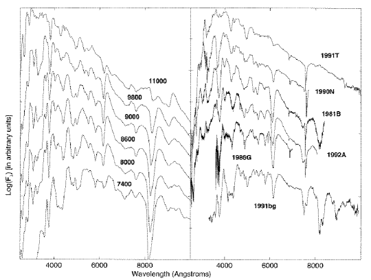
Figure 1: The observed variation in spectra with brightness at maximum light is well reproduced by variation the model temperature in synthetic spectra calculations.

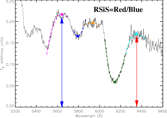
Figure 2: The definition of the spectral ratio $\Re_{SiS}$.

2.1 3-D Explosions

The explosion of a SN Ia is inherently three dimensional since the white dwarf becomes convective shortly before it ignites and the ignition is likely to be off-center. The flame also quickly becomes wrinkled and thus there will be non-spherical compositions. Overall, SNe Ia are basically round, but explosion asymmetries lead to compositional and ionization inhomogeneities. Core-collapse supernovae almost certainly come from asymmetric engine. How important the asymmetry is to spectra formation depends on how much of the hydrogen or helium envelope has been lost and how late one observes the spectrum. Gamma ray bursts are beamed and highly relativistic. And of course AGN are asymmetric and may require general relativity.

3 Detailed Quantitative Spectroscopy

3.1 PHOENIX

PHOENIX is a generalized model atmosphere code, that solves the generalized stellar atmosphere problem in static or moving flows using the fully special relativistic approach. For supernovae with characteristic velocities of 10,000 $\mathrm{km}~{}\mathrm{s}^{-1}$ and maximum velocities of up to 60,000 $\mathrm{km}~{}\mathrm{s}^{-1}$ the exact special relativistic formulation is preferred. PHOENIX is well calibrated on many astrophysical objects including the sun (Short and Hauschildt, 2005), cool stars (Helling et al., 2008), hot stars (Aufdenberg et al., 2006), planets (Hauschildt et al., 2008), novae (Petz et al., 2005), and all types of supernovae (Bongard et al., 2008; Ketchum et al., 2008; Baron et al., 2008, 2007; Knop et al., 2007).

Over the last four years or so we have been developing a fully 3-D version of PHOENIX (Hauschildt and Baron, 2006; Baron and Hauschildt, 2007; Hauschildt and Baron, 2008, 2009; Baron et al., 2009; Chen et al., 2007). We have built this up slowly and carefully making sure to do careful code verification along the way. Fig. 3 shows the results from a spherically symmetric static test case with scattering. This test was especially useful because it showed that our full characteristics method was far superior to a short characteristics method in terms of reproducing the spherical symmetry. Since this model is a sphere in a box, the sphere is surrounded by vacuum and the interpolations needed for the short characteristics method did a very poor job of reproducing the correct results across the opacity discontinuity.

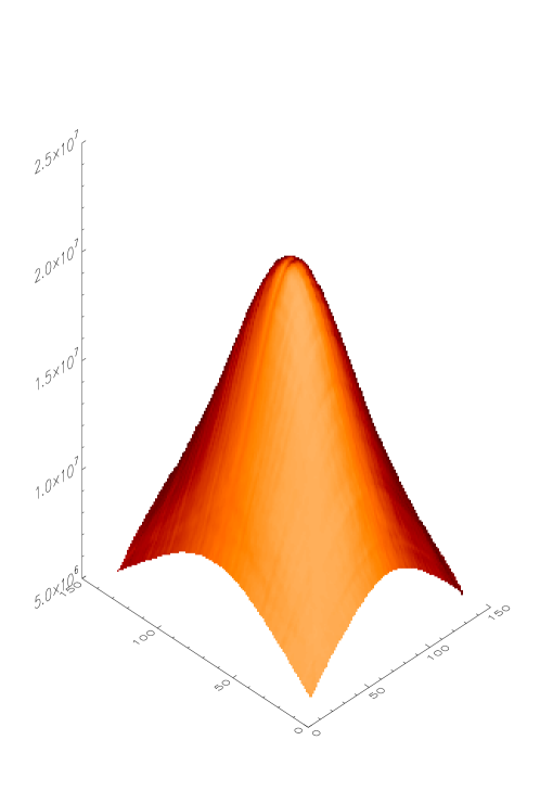
Figure 3: Sphere in a box, mean intensity $J$ is plotted for a a slice through the x-y plane for the case of a scattering continuum with $\epsilon=10^{-4}$.

Figure 4 shows a toy solar model using periodic boundary conditions. The temperature and density structure was taken from the model of Caffau et al. (2007) but the opacity was taken to be proportional to the density and independent of temperature. The thermalization parameter in this calculation was taken to be $\epsilon=1$.

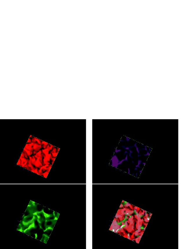
Figure 4: The top left panel shows the continuum, the top right panel the line center, the bottom left the line wing, and the bottom right a composite image.

Our general method is described in detail in Refs (Hauschildt and Baron, 2006; Baron and Hauschildt, 2007; Hauschildt and Baron, 2008, 2009) and is modeled on the methods in our 1-D code (Hauschildt, 1992b; Hauschildt and Baron, 1999, 2004). The mean intensity $J$ is obtained from the source function $S$ by a formal solution of the RTE which is symbolically written using the $\Lambda$-operator $\Lambda$ as

$$J=\Lambda S.$$ (1)

The source function is given by $S=(1-\epsilon)J+\epsilon B$, where $\epsilon$ denotes the thermal coupling parameter and $B$ is Planck’s function.

The $\Lambda$-iteration method, i.e. to solve Eq. 1 by a fixed-point iteration scheme of the form

$${J_{\rm new}}=\Lambda{S_{\rm old}},\quad{S_{\rm new}}=(1-\epsilon){J_{\rm new}}+\epsilon B,$$ (2)

fails in the case of large optical depths and small $\epsilon$. The idea of the ALI or operator splitting (OS) method is to reduce the eigenvalues of the amplification matrix in the iteration scheme (Cannon, 1973) by introducing an approximate $\Lambda$-operator (ALO) ${\Lambda^{*}}$ and to split $\Lambda$ according to

$$\Lambda={\Lambda^{*}}+(\Lambda-{\Lambda^{*}})$$ (3)

and rewrite Eq. 2 as

$${J_{\rm new}}={\Lambda^{*}}{S_{\rm new}}+(\Lambda-{\Lambda^{*}}){S_{\rm old}}.$$ (4)

This relation can be written as Hamann (1987)

$$\left[1-{\Lambda^{*}}(1-\epsilon)\right]{J_{\rm new}}={J_{\rm fs}}-{\Lambda^{*}}(1-\epsilon){J_{\rm old}},$$ (5)

where ${J_{\rm fs}}=\Lambda{S_{\rm old}}$ and ${J_{\rm old}}$ is the current estimate of the mean intensity $J$. Equation 5 is solved to get the new values of ${J}$ which is then used to compute the new source function for the next iteration cycle.

Matrix computations are required in order to solve Eq. 5. In choosing matrix methods one must remember that the inverse of a banded matrix is full. Band matrix solvers require large amounts of memory. This is also the case for parallelized band matrix solvers. Iterative methods (Jordan and Gauss-Seidel) work well and use little memory. Ng acceleration is still very useful. Figure 5 shows that the ALO works well and the Ng acceleration is evident.

Figure 5: Convergence rates of the 3D transfer for line transfer with plane-parallel test structures (label ‘PP’) and the 3D hydro structure (label ‘hydro’). For comparison, the convergence of the $\Lambda$ iteration for plane-parallel continuum transfer is also shown.

4 Moving Atmospheres

For the moving case one must derive the equation of radiative transfer using the techniques of general relativity. The pioneering work in this field was done by Lindquist (Lindquist, 1966). We sketch the development of the solution of the relativistic radiative transfer equation beginning with the work of Mihalas (Mihalas, 1980) and describe the work we have done (Baron et al., 2009; Chen et al., 2007).

4.1 Mihalas’ Method

In his important paper Dimitri Mihalas (Mihalas, 1980) explained why we want to work in the co-moving frame (italics as in original):

The emissivity $\eta$ and opacity $\chi$ depend upon the angle as well as frequency in the inertial frame because of Doppler shifts, aberration, and advection induced by the motion of the material in the frame.

The goal of this section is to rewrite equation (2.1) with all material and radiation-field quantities measured in the comoving frame; in that frame both the opacity and emissivity are isotropic, and can be related directly to proper variables that specify the thermodynamic state of the material. Furthermore, in that frame both the scattering properties of the material and the rate equations describing the mechanisms populating and depopulating its internal energy states are most easily defined…

In our analysis we shall, however, leave both the space and time variables in the inertial frame, as this is the only frame in which synchronism of clocks can be effected, and further this choice obviates the need to develop a metric for accelerated fluid frames (Castor, 1972) which in general can only be done approximately. With this choice of frame we can write exact Lorentz transformations for all the material and radiation-field quantities and use these to develop a transfer equation that will remain valid for relativistic flow in the limit as $v/c\longrightarrow 1$…

In Mihalas (1980) the characteristic equations are written as coupled ordinary differential equations in both the inertial frame spatial coordinate, $r,$ and the co-moving frame momentum space coordinate, $\mu$, i.e.,

$$\frac{dr}{ds_{M}} = \gamma(\mu+\beta),$$

$$\frac{d\mu}{ds_{M}} = \gamma(1-\mu^{2})\left[{1+\mu\frac{\beta}{r}}-\gamma^{2}(\mu+\beta)\frac{d\beta}{dr}\right].$$

From these results of Mihalas a generation of workers in the field have been educated that the characteristics are curved in phase space (see Figure 1 of Reference Mihalas, 1980).

4.2 The Affine Method

Generalizing the method of Mihalas (1980) to 3 spatial dimensions (and thus 6 phase space dimensions) is very difficult. Following the methodology of Mihalas (1980) we would keep all 3 momentum space variables co-moving. Then, in order to keep track of the evolution of those co-moving phase space variables along the characteristics (e.g., $\mu,$ $\phi$), we would have relied on the so-called tetrad formalism (Morita and Kaneko, 1984, 1986; Castor, 2009) which is very complicated for spacetimes with no symmetry or arbitrary flows. For an example, a boost followed by an arbitrary $SO(3)$ rotation is still a valid Lorentz transformation and thus it is difficult to define a consistent frame in the case of arbitrary flows. In Chen et al. (2007) we realized that photons travel along null geodesics (straight lines in flat spacetime), which depends only on the background spacetime, not the velocity distribution of the flow, and consequently is either known analytically or can be numerically solved before we solve the RTE. The so-called characteristics in phase space are just the ‘unique’ lifting of the geodesics in the $4$-D spacetime manifold to the $8$-D tangent bundle of the spacetime manifold (Lindquist, 1966; Ehlers, 1971). The apparent curvature of the characteristics in (Mihalas, 1980) is due to the selection of phase space coordinates. To avoid the complications induced by the use of the tetrad formalism, we found that we could work in a very special co-moving frame where only the wavelength of the photon is measured by a co-moving observer (which differs from the inertial frame value by only a Doppler factor and is thus easily calculated), the other two momentum directions are measured in the observer’s frame (which in flat spacetime are constants). This is not a giant leap, since in the case of Mihalas (1980) the transfer equation is solved in a mixed frame, where the spatial variables are Eulerian, but the two momentum variables $\mu$ and $\lambda$ are measured by a co-moving observer. Figure 6 illustrates the characteristics for a Cartesian grid.

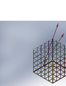
Figure 6: Characteristics are straight lines in flat spacetime and they begin at a boundary point and traverse the computational volume with a constant direction measured in the observer’s frame.

The above considerations lead to a radiative transfer equation given by

$$\left.\frac{\partial I_{\lambda}}{\partial s}\right|_{\lambda}+a(s)\lambda\frac{\partial I_{\lambda}}{\partial\lambda}=-[\chi_{\lambda}f(s)+5a(s)]I_{\lambda}+\eta_{\lambda}f(s).$$ (6)

where the notation is the same as in Baron et al. (2009).

The evaluation of $I_{\lambda}$ in this mixed frame makes it quite easy to solve the scattering problem in the co-moving frame. To get the co-moving $J_{\lambda},$ we need to integrate the (co-moving) specific intensity $I_{\lambda}(\bf{r},\hat{\bf n})$ over the co-moving solid angle element $d\Omega.$ Since $I_{\lambda}(\bf{r},\hat{\bf n})$ is given in terms of the inertial frame direction $\hat{\bf n},$ it is desirable to transform the integral into one over the inertial frame solid angle element $d\Omega_{0},$ this causes no difficulty since

$$d\Omega = (\gamma[1-\mathbf{\beta\cdot n}])^{-2}d\Omega_{0}$$ (7)

$$= f(s)^{-2}d\Omega_{0}.$$

Using Eq. 7, $J_{\lambda}$ in the co-moving frame can be expressed as

$$J_{\lambda}=\int I_{\lambda}({\bf r},{\hat{\bf n}})f(s)^{-2}d\Omega_{0}$$ (8)

where $I_{\lambda}({\bf r},{\hat{\bf n}})$ is expressed in the “funny frame” that comes from solving Eq. 6.

We have implemented this method in spherical coordinates for the case of homologous flows (Baron et al., 2009). It is important to verify that the code gives the correct results in a case that can be tested. Luckily, we can compare the results for a spherically symmetric test with those of our well-tested 1-D code, which uses the Mihalas’ method and not the affine method. Figure 7 compares the results for the mean intensity $J$ in the co-moving frame of the 1-D code (dots) and the 3-D (solid lines) at each voxel at a given radius for differing maximum velocities. No scaling is performed between the two calculations. The agreement is excellent and the 3-D code does a very good job of reproducing spherical symmetry. This also shows that there is no problem in the interpretation of our frame. Figure 8 shows similar results for a scattering line in the co-moving frame. Figure 9 shows the flux in the observer’s frame reproduces the expected P-Cygni profile. Figure 10 shows that the code parallelizes quite well in terms of resolution. The scaling test has each processor working on the same number of characteristics as the number of momentum space angles is increased. The 14% cost is reasonable given the increased communication overhead as one goes from 256 to 16,384 processors.

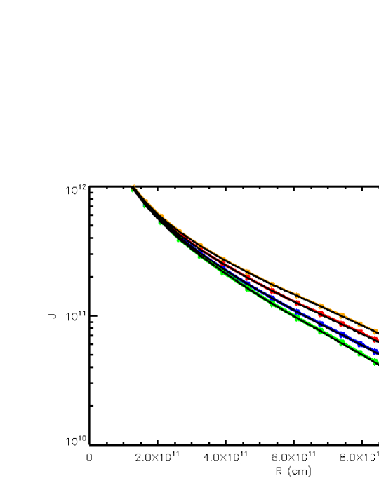
Figure 7: The results of 1-D calculations are compared with 3-D calculations for $\beta_{max}=(0.03,0.33,0.67,0.87)$.

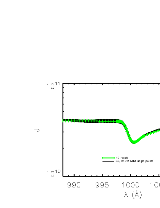
Figure 8: The mean intensity of a line in the co-moving frame for a line with $\epsilon=0.1$, $\beta_{max}=0.03$. The solid lines are the 3-D result and the plus signs are the 1-D results.

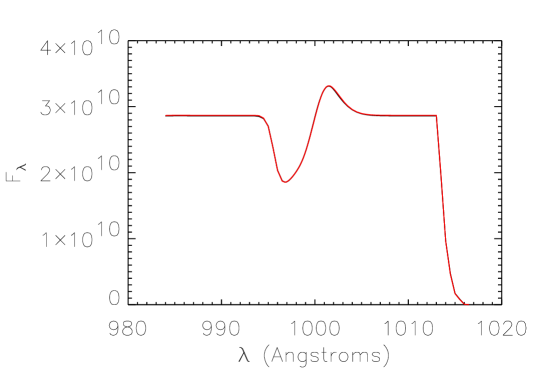
Figure 9: The line shown in Fig 8 transformed to the observer’s frame gives the expected P-Cygni profile.

Figure 10: Wall-clock time for $\epsilon=0.1$ as a function of angular resolution/number of CPUs.

5 Summary

PHOENIX now includes tested 3-D fully relativistic radiative transfer with homologous flows. Including arbitrary flows is a computational, not an algorithmic challenge (Baron and Hauschildt, 2004; Knop et al., 2009) and we are working on this. The next step is to go beyond test problems to a full production code. We expect progress from the inter-comparison of new datasets of nearby supernovae with 3-D hydro models and synthetic spectroscopy. The affine method is extremely easy to implement and can be applied to radiation hydro codes. Happy birthday Dimitri!

References

- Mihalas (1980) D. Mihalas, ApJ 237, 574 (1980).
- Mihalas and Kunasz (1978) D. Mihalas, and P. Kunasz, ApJ 219, 635 (1978).
- Mihalas et al. (1976a) D. Mihalas, P. Kunasz, and D. Hummer, ApJ 203, 647 (1976a).
- Mihalas et al. (1976b) D. Mihalas, P. Kunasz, and D. Hummer, ApJ 206, 515 (1976b).
- Mihalas et al. (1976c) D. Mihalas, P. Kunasz, and D. Hummer, ApJ 210, 419 (1976c).
- Mihalas et al. (1975) D. Mihalas, P. Kunasz, and D. Hummer, ApJ 202, 465 (1975).
- Hauschildt (1993) P. H. Hauschildt, JQSRT 50, 301 (1993).
- Hauschildt (1992a) P. H. Hauschildt, ApJ 398, 224 (1992a).
- Hauschildt (1992b) P. H. Hauschildt, JQSRT 47, 433 (1992b).
- Hauschildt and Baron (1999) P. H. Hauschildt, and E. Baron, J. Comp. Applied Math. 109, 41 (1999).
- Hauschildt and Baron (2004) P. H. Hauschildt, and E. Baron, Mitteilungen der Mathematischen Gesellschaft in Hamburg 24, 1 (2004).
- Phillips (1993) M. M. Phillips, ApJ 413, L105 (1993).
- Phillips et al. (1999) M. M. Phillips, P. Lira, N. B. Suntzeff, R. A. Schommer, M. Hamuy, and J. Maza, AJ 118, 1766–1776 (1999).
- Khokhlov et al. (1993) A. Khokhlov, E. Müller, and P. Höflich, A&A 270, 223 (1993).
- Höflich and Khokhlov (1996) P. Höflich, and A. Khokhlov, ApJ 457, 500 (1996).
- Nugent et al. (1995) P. Nugent, M. Phillips, E. Baron, D. Branch, and P. Hauschildt, ApJ 455, L147 (1995).
- Kasen and Woosley (2007) D. Kasen, and S. E. Woosley, ApJ 656, 661–665 (2007).
- Filippenko (1997) A. V. Filippenko, Ann. Rev. Astr. Ap. 35, 309 (1997).
- Goldhaber et al. (2001) G. Goldhaber, et al., ApJ 558, 359 (2001).
- Jha et al. (2007) S. Jha, A. G. Riess, and R. P. Kirshner, ApJ 659, 122–148 (2007).
- Riess et al. (1998) A. Riess, et al., AJ 116, 1009 (1998).
- Perlmutter et al. (1999) S. Perlmutter, et al., ApJ 517, 565 (1999).
- Sullivan et al. (2009) M. Sullivan, R. S. Ellis, D. A. Howell, A. Riess, P. E. Nugent, and A. Gal-Yam, ApJ 693, L76–L80 (2009).
- Garnavich et al. (2004) P. M. Garnavich, et al., ApJ 613, 1120 (2004).
- Bongard et al. (2006) S. Bongard, E. Baron, G. Smadja, D. Branch, and P. Hauschildt, ApJ 647, 480 (2006).
- Bailey et al. (2009) S. Bailey, G. Aldering, P. Antilogus, C. Aragon, C. Baltay, S. Bongard, C. Buton, M. Childress, N. Chotard, Y. Copin, E. Gangler, S. Loken, P. Nugent, R. Pain, E. Pecontal, R. Pereira, S. Perlmutter, D. Rabinowitz, G. Rigaudier, K. Runge, R. Scalzo, G. Smadja, H. Swift, C. Tao, R. C. Thomas, and C. Wu, A&A in press (2009), 0905.0340.
- Short and Hauschildt (2005) C. I. Short, and P. H. Hauschildt, ApJ 618, 926–938 (2005).
- Helling et al. (2008) C. Helling, A. Ackerman, F. Allard, M. Dehn, P. Hauschildt, D. Homeier, K. Lodders, M. Marley, F. Rietmeijer, T. Tsuji, and P. Woitke, MNRAS 391, 1854–1873 (2008).
- Aufdenberg et al. (2006) J. P. Aufdenberg, N. D. Morrison, P. H. Hauschildt, and S. J. Adelman, “The Photosphere and Stellar Wind of Deneb (A2 Ia) in the Far Ultraviolet,” in Astrophysics in the Far Ultraviolet: Five Years of Discovery with FUSE, edited by G. Sonneborn, H. W. Moos, and B.-G. Andersson, 2006, vol. 348 of Astronomical Society of the Pacific Conference Series, pp. 124–+.
- Hauschildt et al. (2008) P. H. Hauschildt, T. Barman, and E. Baron, Physica Scripta Volume T 130, 014033–+ (2008).
- Petz et al. (2005) A. Petz, P. H. Hauschildt, J.-U. Ness, and S. Starrfield, A&A 431, 321–328 (2005).
- Bongard et al. (2008) S. Bongard, E. Baron, G. Smadja, D. Branch, and P. Hauschildt, ApJ 687, 456 (2008).
- Ketchum et al. (2008) W. Ketchum, E. Baron, and D. Branch, ApJ 674, 371–377 (2008).
- Baron et al. (2008) E. Baron, D. J. Jeffery, D. Branch, E. Bravo, D. Garcia-Senz, and P. H. Hauschildt, ApJ 672, 1038 (2008).
- Baron et al. (2007) E. Baron, D. Branch, and P. H. Hauschildt, ApJ 662, 1148 (2007).
- Knop et al. (2007) S. Knop, P. H. Hauschildt, E. Baron, and S. Dreizler, A&A 469, 1077–1081 (2007).
- Hauschildt and Baron (2006) P. H. Hauschildt, and E. Baron, A&A 451, 273 (2006).
- Baron and Hauschildt (2007) E. Baron, and P. H. Hauschildt, A&A 468, 255 (2007).
- Hauschildt and Baron (2008) P. H. Hauschildt, and E. Baron, A&A 490, 873 (2008).
- Hauschildt and Baron (2009) P. H. Hauschildt, and E. Baron, A&A 498, 981 (2009).
- Baron et al. (2009) E. Baron, P. H. Hauschildt, and B. Chen, A&A 498, 987 (2009).
- Chen et al. (2007) B. Chen, R. Kantowski, E. Baron, S. Knop, and P. Hauschildt, MNRAS 380, 104 (2007).
- Caffau et al. (2007) E. Caffau, M. Steffen, L. Sbordone, H.-G. Ludwig, and P. Bonifacio, A&A 473, L9–L12 (2007).
- Cannon (1973) C. J. Cannon, JQSRT 13, 627 (1973).
- Hamann (1987) W.-R. Hamann, “Numerical Radiative Transfer,” Cambridge Univ. Press, Cambridge, 1987, p. 35.
- Lindquist (1966) R. Lindquist, Annals of Physics 37, 487 (1966).
- Castor (1972) J. I. Castor, ApJ 178, 779 (1972).
- Morita and Kaneko (1984) K. Morita, and N. Kaneko, Ap&SS 107, 333 (1984).
- Morita and Kaneko (1986) K. Morita, and N. Kaneko, Ap&SS 121, 105 (1986).
- Castor (2009) J. I. Castor, “Toward a Fully Consistent Radiation Hydrodynamics,” in Recent Directions In Astrophysical Quantitative Spectroscopy And Radiation Hydrodynamics, edited by I. Hubeny, J. Stone, and M. Norman, American Inst. of Physics, New York, 2009, this volume.
- Ehlers (1971) J. Ehlers, “General Relativity and Kinetic Theory,” in General Relativity and Cosmology, Proceedings of the International School of Physics “Enrico Fermi”, edited by R. K. Sachs, Academic Press, London, 1971, p. 1.
- Baron and Hauschildt (2004) E. Baron, and P. H. Hauschildt, A&A 427, 987 (2004).
- Knop et al. (2009) S. Knop, P. H. Hauschildt, and E. Baron, A&A 496, 295 (2009).