Microscopic Structural Relaxation in a Sheared Supercooled Colloidal Liquid

Abstract

The rheology of dense amorphous materials under large shear strain is not fully understood, partly due to the difficulty of directly viewing the microscopic details of such materials. We use a colloidal suspension to simulate amorphous materials, and study the shear-induced structural relaxation with fast confocal microscopy. We quantify the plastic rearrangements of the particles in several ways. Each of these measures of plasticity reveals spatially heterogeneous dynamics, with localized regions where many particles are strongly rearranging by these measures. We examine the shapes of these regions and find them to be essentially isotropic, with no alignment in any particular direction. Furthermore, individual particles are equally likely to move in any direction, other than the overall bias imposed by the strain.

I Introduction

Many common materials have an amorphous structure, such as shaving cream, ketchup, toothpaste, gels, and window glass Angell et al. (2000); Coussot and Gaulard (2005); Ubbink et al. (2008); Mezzenga et al. (2005). In some situations these are viscous liquids, for example when window glass is heated above the glass transition temperature, or a shaving cream foam that has been diluted by water to become a liquid with bubbles in it. In other situations these are viscoelastic or elastic solids, such as gels and solid window glass Liu and Nagel (1998). For solid-like behavior, when a small stress is applied, the materials maintain their own shapes; at larger stresses above the yield stress, they will start to flow Coussot et al. (2002); Huang et al. (2005); Merkt et al. (2004). Understanding how these materials yield and flow is important for the processing of these materials, and understanding their strength in the solid state Spaepen (1977); Sheng et al. (2007); Schuh et al. (2007).

A particularly interesting system to study is a colloidal suspension. These consist of micron or submicron sized solid particles in a liquid. At high particle concentration, macroscopically these are pastes and thus of practical relevance Coussot et al. (2002). Additionally, for particles with simple hard-sphere like interactions, colloidal suspensions also serve as useful model systems of liquids, crystals, and glasses Pusey and van Megen (1986); Haw (2002); Suresh (2006); Schall et al. (2007). Such colloidal model systems have the advantage that they can be directly observed with microscopy Habdas and Weeks (2002); Prasad et al. (2007); Elliot and Poon (2001). Our particular interest in this paper is using colloidal suspensions to model supercooled and glassy materials. The control parameter for hard sphere systems is the concentration, expressed as the volume fraction $\phi$, and the system acts like a glass for $\phi>\phi_{g}\approx 0.58$. The transition is the point where particles no longer diffuse through the sample; for $\phi<\phi_{g}$ spheres do diffuse at long times, although the asymptotic diffusion coefficient $D_{\infty}$ decreases sharply as the concentration increases van Megen and Pusey (1991); Speedy (1998); Brambilla et al. (2009). The transition at $\phi_{g}$ occurs even though the spheres are not completely packed together; in fact, the density must be increased to $\phi_{\rm RCP}\approx 0.64$ for “random-close-packed” spheres O’Hern et al. (2003); Bernal (1964); Torquato et al. (2000); Donev et al. (2004); O’Hern et al. (2004) before the spheres are motionless. Prior work has shown remarkable similarities between colloidal suspensions and conventional molecular glasses Pusey and van Megen (1986); van Megen and Pusey (1991); van Blaaderen and Wiltzius (1995); van Megen and Underwood (1993, 1994); Snook et al. (1991); Bartsch et al. (1993); Bartsch (1995); Mason and Weitz (1995).

One important unsolved problem related to amorphous materials is to understand the origin of their unique rheological behavior under shear flow. Early in the 70’s, theory predicted the existence of “flow defects” beyond yielding Spaepen (1977), later termed shear transformation zones (STZ) Falk and Langer (1998). These microscopic motions result in plastic deformation of the sheared samples Goyon et al. (2008); Bocquet et al. (2009). Simulations later found STZs by examining the microscopic local particle motions Schuh et al. (2007); Yamamoto and Onuki (1997); Miyazaki et al. (2004). Recently fast confocal microscopy has been used to examine the shear of colloidal suspensions Besseling et al. (2007), and STZ’s have been directly observed Schall et al. (2007). This provided direct evidence to support theoretical work on STZ’s Spaepen (1977); Maeda and Takeuchi (1981); Falk and Langer (1998); Shi and Falk (2005).

However, questions still remain. First, most of the prior work has focused on the densest possible samples, at concentrations which are glassy ($\phi>\phi_{G}$) Besseling et al. (2007); Schall et al. (2007). Given that the macroscopic viscosity of colloidal suspensions change dramatically near and above $\phi_{G}$ Cheng et al. (2002), it is of interest to study slightly less dense suspensions under shear, for which rearrangements might be easier Weeks et al. (2000). In this paper, we present such results. Second, prior investigations of sheared amorphous materials have used a variety of different ways to quantify plastic deformation Wang et al. (2006); Utter and Behringer (2008); Besseling et al. (2007); Schall et al. (2007). In this paper, we will compare and contrast plastic deformations defined in several different ways. While they do capture different aspects of plastic deformation, we find that some results are universal. In particular, in a sheared suspension, there are three distinct directions: the strain velocity, the velocity gradient, and the direction mutually perpendicular to the first two (the “vorticity” direction). We find that plastic deformations are isotropic with respect to these three directions, apart from the trivial anisotropy due to the velocity gradient. The deformations are both isotropic in the sense of individual particle motions, and in the sense of the shape of regions of rearranging particles.

II Experimental Methods

The experimental setup of our shear cell is shown in Fig. 1 and is similar to that described in Refs. Petekidis et al. (2002); Besseling et al. (2007). The glass plates are 15 mm in diameter, and to the top plate is glued a small piece of glass with dimensions 5 mm$\times$1 mm, with the long dimension oriented in the direction of motion $x$. The purpose of this piece of glass is to decrease the effective gap size. Between the plates are three ball bearings, used to control the gap size; for all of our data, we maintain a gap size of $H=130$ $\mu$m. Over the 5 mm length of the small pieces of glass, the gap varies by no more than 15 $\mu$m; over the narrower dimension of the small pieces of glass, the gap varies by no more than 10 $\mu$m. Thus, overall the sample is between two plates which are parallel to within 1% and in the direction of shear, they are parallel to within 0.3%.

A droplet of the sample (volume $\sim$200 $\mu$l) is placed between the two pieces of glass. The top plate is free to move in the $x$ direction, and the bottom plate is motionless. The shear rate is controlled by a piezo-electric actuator (Piezomechanik GmbH Co.) driven by a triangular wave signal with a period ranging from $T=150$ to 450 s and an amplitude of $A=175$ $\mu$m. Thus we achieve strains of $\gamma_{0}=A/H=1.4$. Prior to taking data, we allow the shear cell to go through at least one complete period, but usually not more than three complete periods.

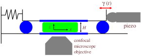
Figure 1: (Color online) Sketch of the shear cell. A fluorescent sample (gray, green online) is put between two parallel glass plates (dark gray, blue online) with gap $H$ set by three ball bearings, two of which are shown. The top plate is movable, controlled by a piezo motor driven by a triangular wave. The bottom plate is fixed, and the confocal microscope takes images from underneath. Note the definition of the coordinate system, where $x$ is in the velocity direction and $z$ is in the velocity gradient direction.

Our samples (Fig. 2) are poly(methyl methacrylate) colloids sterically stabilized with poly-12-hydroxystearic acid Antl et al. (1986). These particles are suspended in a mixture of 85% cyclohexybromide and 15% decalin by weight. This mixture matches both the density and the index of refraction of the particles. To visualize the particles, they are dyed with rhodamine $6G$ Dinsmore et al. (2001). The particles have a radius $a=1.05\pm 0.04$ $\mu$m, with the error bar indicating the uncertainty in the mean diameter; additionally the particles have a polydispersity of no more than 5% (as these particles can crystallize fairly easily) Pusey and van Megen (1986); Auer and Frenkel (2001); Henderson et al. (1996); Schöpe et al. (2007).

In this work we study several samples with volume fractions $\phi$ between 0.51 and 0.57. Thus, our samples are quite dense liquids, comparable to prior work with “supercooled” colloidal liquids Pusey and van Megen (1986); Weeks et al. (2000). The differences in volume fraction between samples are certain to within $\pm 0.01$, and the absolute volume fraction has a systematic uncertainty of $\pm 0.06$ due to the uncertainty of the particle radius $a$. However, none of our samples appear glassy, and thus we are confident our maximum volume fraction is less than $\sim 0.6$. While the particles in decalin behave as hard-spheres, in our solvent mixture they carry a slight charge. This does not seem to affect the phase behavior dramatically at high volume fractions such as what we consider in this work; see for example Gasser et al. (2001); Hernández-Guzmán and Weeks (2009).

To characterize the relative importance of Brownian motion and the imposed strain field, we can compute the modified Peclet number, $Pe^{\star}=\dot{\gamma}a^{2}/2D_{\infty}$, where $D_{\infty}$ is the long time diffusion coefficient of the quiescent sample. We measure $D_{\infty}$ from mean square displacement data taken from the quiescent sample with the same volume fraction. The large $\Delta t$ data for the mean square displacement can be fit using $\langle\Delta x^{2}\rangle=2D_{\infty}\Delta t$. Roughly, $a^{2}/2D_{\infty}$ reflects the average duration a particle is caged by its neighbors in the dense suspension.

$\dot{\gamma}$ is the imposed strain rate $2A/(HT)$, and $a$ is the particle size. The extra factor of 2 in $\dot{\gamma}$ is because we use a triangle wave, and thus the half period sets the strain rate. For our samples, we find $D_{\infty}\approx 5\times 10^{-4}$ $\mu$m${}^{2}/$s, and we have $\dot{\gamma}$ ranging from 0.0060 to 0.0180 s^-1; thus $Pe^{\star}\approx 7-20$. Given that $Pe^{\star}>1$, the implication is that the motions we will observe are primarily caused by the strain, rather than due to Brownian motion. We use the modified Peclet number based on $D_{\infty}$ rather than the bare Peclet number based on the dilute-limit diffusivity $D_{0}$, as we will focus our attention on the dynamics at long time scales, which we will show are indeed shear-induced.

Shear-induced crystallization has been found in previous work Haw et al. (1998a); Duff and Lacks (2007). As we wish to focus on the case of sheared amorphous materials, we check our data to look for crystalline regions using standard methods which detect ordering Gasser et al. (2001); Hernández-Guzmán and Weeks (2009); Dullens et al. (2006); ten Wolde et al. (1996); Steinhardt et al. (1983). Using these methods, we find that particles in apparently crystalline regions comprise less than 3% of the particles in each of our experiments, and are not clustered, suggesting that the apparently crystalline regions are tiny. This confirms that our samples maintain amorphous structure over the time scale of our experiments, although perhaps if we continued the shearing over many more cycles we would find shear-induced crystallization.

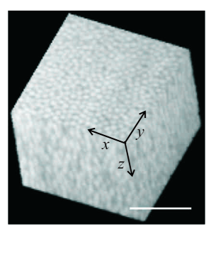
Figure 2: A 20$\times$20$\times$20 $\mu$m³ image of a supercooled colloidal liquid taken 15 $\mu$m away from the fixed bottom plate by our confocal microscope in less than 1 s. The scale bar represents 10 $\mu$m.

We use a confocal microscope to image our sample (the “VT-Eye”, Visitech), using a 100$\times$ oil lens (numerical aperture = 1.40) van Blaaderen et al. (1992); Dinsmore et al. (2001); Prasad et al. (2007). A 3D image with a volume 50$\times$50$\times$20 $\mu$m³ is acquired in less than 2 s; these images contain about 6000 particles. The 3D image is $256\times 256\times 100$ pixels, so approximately 0.2 $\mu$m per pixel in each direction. Figure 2 shows a representative image from a somewhat smaller volume. The 2 s acquisition time is several orders of magnitude faster than the diffusion for particles in our high volume fraction sample. To avoid any boundary effects Shereda et al. (2008), we scan a volume at least 20 $\mu$m away from the bottom plate. Particle positions are determined with an accuracy of $0.05$ $\mu$m in $x$ and $y$, and $0.1$ $\mu$m in $z$. This is done by first spatially filtering the 3D image with a bandpass filter designed to remove noise at high and low spatial frequencies, and then looking for local maxima in the image intensity Crocker and Grier (1996). Our tracking algorithm is similar to prior work Crocker and Grier (1996); Dinsmore et al. (2001); Besseling et al. (2009), where we first identify particles within each 3D image, next remove the overall average shear-induced motion from all of the particles, then track the particles in the “co-shearing” reference frame using conventional techniques Crocker and Grier (1996), and finally add back in the shear-induced motion that was previously removed. This is similar to the “Iterated CG tracking” method described in Ref. Besseling et al. (2009). The key idea of this tracking is that particles should not move more than an inter-particle spacing between each image; this condition is satisfied in the co-shearing reference frame.

Due to the strain, particles that start near one face of the imaging volume are carried outside the field of view, while on the opposite face new particles are brought inside. Thus, for larger strains, the total number of particles viewed for the entire duration diminishes. For the data discussed in this work, we consider both instantaneous quantities and quantities averaged over the entire half-cycle of strain. For the former, we view $\sim 5500$ particles, while for the latter, we typically can follow $\sim 3000$ particles, which limits our statistics slightly.

III Results

III.1 Locally observed strain

Our goal is to understand if the local shear-induced motion is isotropic in character. However, first we seek to understand and quantify the more global response of our sheared samples.

When shearing disordered materials or complex fluids, one often finds shear localization or shear banding, due to the nonlinear yielding and relaxation in local regions Huang et al. (2005); Coussot et al. (2002); Chan et al. (2004); Lauridsen et al. (2004). To check for this in our data, we start by taking 3D images under the applied shear rate $\dot{\gamma}_{\rm macro}=0.016$ s^-1 over a very large range in $z$, from 0 to 70 $\mu$m away from the bottom plate, almost half of the gap between two shearing plates. To allow us to visualize more clearly over such a large depth, we dilute the dye concentration by mixing dyed and undyed colloids at a number ratio of around 1$:$80 and keeping the desired volume fraction $\phi\approx 0.50$. Our sample does indeed form a shear band, as shown in Fig. 3, which shows the particle velocity $v_{x}$ in the direction of the shear as a function of the depth $z$. The velocity changes rapidly with $z$ in the range $0<z<20$ $\mu$m, and then more slowly for $z>20$ $\mu$m; thus much of the shear occurs adjacent to the stationary plate at $z=0$ $\mu$m, similar to prior work which found shear adjacent to one of the walls Cohen et al. (2006); Huang et al. (2005); Coussot et al. (2002); Chan et al. (2004); Lauridsen et al. (2004). Furthermore, the velocity profile is relatively stable during the course of the half-period, as seen by the agreement between the velocity profiles taken at different times during this half period (different lines in Fig. 3. Thus, the shear band develops quickly inside the supercooled colloidal liquid, and remains fairly steady under the constant applied strain rate. The location and size of the shear band varies from experiment to experiment.

Given the existence of a shear band, the applied strain is not always the local strain. In this work we wish to focus on the motion induced by a local strain, rather than the global formation of shear bands. Thus, for all data sets presented below, we always calculate the local instantaneous strain rate $\dot{\gamma}_{\rm meso}(t)=\frac{v_{x}(z+\Delta z,t)-v_{x}(z,t)}{\Delta z}$. Here $\Delta z=20$ $\mu$m is the height of the imaged volume. Related to $\dot{\gamma}_{\rm meso}$, we can calculate the total local applied strain by integrating $\dot{\gamma}_{\rm meso}(t)$:

$$\gamma_{\rm meso}(t)=\int^{t}_{0}\dot{\gamma}_{\rm meso}(t^{\prime})dt^{\prime}.$$ (1)

Furthermore, we verify that for each data set considered below, $v_{x}(z)$ varies linearly with $z$ within the experimental uncertainty, and thus $\dot{\gamma}_{\rm meso}$ is well-defined, even if globally it varies (Fig. 3).

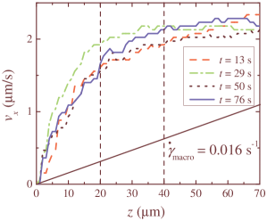
Figure 3: (Color online) Shear profile $v_{x}(z)$ within a 50$\times$50$\times$70 $\mu$m³ volume, measured at different times during one half period $T/2=84$ s. The total macroscopic strain applied in 84 s is 1.35. The sample has a volume fraction $\phi\approx 0.50$, and the global applied shear rate is $\dot{\gamma}_{\rm macro}=0.016$ s^-1 controlled by the piezo motor. If there was not a shear band, one would expect to observe a linear velocity profile as indicated by the lower thick diagonal line. The four curves represent different times during the half period as indicated. Note that these data are obtained using a coarse-grained image velocimetry method Besseling et al. (2009), rather than particle tracking. Here we take rapid images over the full volume with a spacing of $z=1$ $\mu$m in the vertical direction. For each value of $z$, we cross-correlate subsequent images to obtain a mean instantaneous velocity $v_{x}$ with a resolution of 0.05 $\mu$m/s, set by the pixel size and the time between images. See Ref. Besseling et al. (2009) for further details.

While the shape of the shear band is essentially constant (Fig. 3), in many cases the local strain rate varies slightly with time. As our forcing is a triangle wave, over any given half cycle the global applied strain rate is a constant. We can measure the local strain rate for each data set; a typical example is shown in Fig. 4. This figure shows the local instantaneous measured strain rate within the region $20$ $\mu$m $<z<40$ $\mu$m, over one full period. After the shearing starts, $\dot{\gamma}_{\rm meso}$ quickly rises up to 0.015 s^-1, implying that the shear band has formed. Subsequently, the local strain rate continues to increase up to 0.030 s^-1 over the rest of the half period. The small fluctuations of $\dot{\gamma}_{\rm meso}$ are due to the microscopic rearrangements of particles, which can be somewhat intermittent. Given that the local instantaneous strain rate is not constant (despite the constant applied strain rate), we will characterize our data sets by the time averaged local strain rate defined as

$$\bar{\dot{\gamma}}_{\rm meso}=\frac{\gamma_{\rm meso}(t)}{t}$$ (2)

typically using $t=T/2$, the half period of the strain. That is, we consider $\bar{\dot{\gamma}}_{\rm meso}$ as one key parameter characterizing each data set, although we will show that we see little dependence on this parameter. In the rest of the paper, the choice $t=T/2$ will be assumed, except where noted when we wish to characterize the mesoscopic strain for time scales shorter than $T/2$.

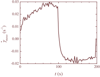
Figure 4: A typical example of a measured local instantaneous shear rate over one period of shearing in a gap of 20$-$40 $\mu$m away from the fixed bottom plate. The sample has volume fraction $\phi=0.51$, the applied strain rate is $\dot{\gamma}_{\rm macro}=0.013$ s^-1, and the period is $T=200$ s.

At this point, we have defined the key control parameters, which are measured from each experimental data set: the strain rate $\bar{\dot{\gamma}}_{\rm meso}$ and the strain amplitude $\gamma_{\rm meso}$. We next consider how these variables relate to the magnitude of the shear-induced particle motion.

III.2 Individual particle motions

Because of our large local strains (measured to be $\gamma_{\rm meso}>0.3$ for all cases), we observe significant particle motion, as shown Fig. 5(a,b). In the laboratory reference frame, the microscopic velocity gradient is obvious either in the raw trajectories [Fig. 5(a)] or in the large displacements [Fig. 5(b)] measured between the beginning and end of the half period. However, in a sense, much of this motion is “trivial”; we wish to observe what nontrivial local rearrangements are caused by the strain. To do this, we consider the non-affine motion by removing averaged particle displacements at the same depth $z$ from the real trajectories of particles Besseling et al. (2007); Wang et al. (2006); Lemaître and Caroli (2007); Miyazaki et al. (2004); Maloney and Robbins (2008),

$$\tilde{x}_{i}(t)=x_{i}(t)-\int^{t}_{0}\dot{\gamma}_{\rm meso}(t^{\prime})z_{i}(t^{\prime})dt^{\prime}$$ (3)

where the removed integral represents the shearing history of the particle $i$. To be clear, the shearing history is based on the average motion within the entire imaged region, and the remaining motion of particle $i$ is caused by interactions with neighboring particles due to the shear. This motion is shown in Fig. 5(c), showing the $\tilde{x}z$ plane rather than the $xz$ plane; the particles move shorter distances. Their overall displacements in this “de-sheared” reference frame are shown in Fig. 5(d). A few trajectories are up to 2 $\mu$m long, comparable to the particle diameter. These non-affine displacements shown in Fig. 5(d) are much smaller than the raw displacements of Fig. 5(b), but much larger than thermally activated Brownian motion, which takes more than 1000 s to diffuse over a 1 $\mu$m distance in our dense samples (comparable to the particle radius $a$). These non-affine motions $\tilde{x}$ reflect shear-induced plastic changes inside the structure.

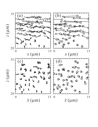
Figure 5: Trajectories of colloids in an $xz$ slice (5 $\mu$m thick in the $y$ direction), see Fig. 1 for the coordinate axes. The sample has $\phi=0.51$, and the data shown correspond to a locally measured accumulated strain $\gamma_{\rm meso}=0.43$ over 45 s of data, so the effective strain rate is $\bar{\dot{\gamma}}_{\rm meso}=\gamma_{\rm meso}/\Delta t=0.0096$ s^-1. (a) Trajectories in a reference frame co-moving with the average velocity $v_{x}(z=20$ $\mu$m$)$. (b) Displacements corresponding to data from panel (a), where the start point of each particle is marked with a circle and the end point is marked with an arrowhead. (c) The same data, but with the affine motion removed; this is the $\tilde{x}z$ plane. (d) Displacements corresponding to panel (c).

To quantify the amount of this non-affine motion $\tilde{x}$, one could calculate the mean squared displacements (MSD) often defined as

$$\langle\Delta\tilde{x}^{2}\rangle(\Delta t)=\langle(\tilde{x}_{i}(t+\Delta t)-\tilde{x}_{i}(t))^{2}\rangle_{i,t}$$ (4)

where the angle brackets indicate an average over time $t$, as well as particles $i$. Thus this identity assumes that environmental conditions remain the same for all the time, since it does not depend on $t$. However, as shown by Fig. 4, the shear rate $\dot{\gamma}_{\rm local}(t)$ depends on the time. Therefore, we use an alternate formulation

$$\langle\Delta\tilde{x}^{2}\rangle(t)=\langle(\tilde{x}_{i}(t)-\tilde{x}_{i}(t=0))^{2}\rangle_{i}$$ (5)

where the angle brackets only indicate an average over particles, and $t$ is the time since the start of a half period of shear. Figure 6(a) shows mean squared displacement (MSD) of the non-affine motion $\Delta\tilde{r}^{2}=\Delta\tilde{x}^{2}+\Delta y^{2}+\Delta z^{2}$ as a function of $t$ for five different experiments with different strain rates $\bar{\dot{\gamma}}_{\rm meso}$, from 0.02 to 0.006 s^-1. In each case the curves nearly reach a slope of 1 on the log-log plot, indicating that shear quickly facilitates particles’ rearrangements. The magnitude of the motion is $\Delta\tilde{r}^{2}\approx 1$ $\mu$m², indicating that the original structure is mostly lost Weeks and Weitz (2002).

Figure 6(a) also shows that $\Delta\tilde{r}^{2}$ is larger for faster strain rates at the same $t$. We find that this motion is determined by the accumulated strain, as shown in Fig. 6(b) by replotting the MSD as a function of $\gamma_{\rm meso}$ (Eqn. 1). In this graph, the curves are grouped closer together and there is no obvious dependence on $\bar{\dot{\gamma}}_{\rm meso}$.

It suggests that the accumulated strain is an important parameter in the structural relaxation, which was also found in previous work on shear transformation zones Delogu (2008); Maloney and Robbins (2008), and is similar behavior to that seen for athermal sheared systems Pine et al. (2005). Additionally, Fig. 6(b) shows that the slopes of the curves are close to 1 when $\gamma_{\rm meso}>0.1$, confirming that the accumulated strain in our experiments is large enough to rearrange the original structure in a supercooled colloidal liquid. We stress that the rough agreement between the curves seen in Fig. 6(b) is based on the locally measured applied strain, and not the macroscopically applied strain.

An earlier study of steady shear applied to colloidal glasses by Besseling et al. Besseling et al. (2007) found that the diffusion time scale $\tau$ scaled as $\dot{\gamma}^{-0.8}$, and simulations also found power law scaling Yamamoto and Onuki (1997); Miyazaki et al. (2004). The collapse of our MSD curves [Fig. 6(b)] seems to imply $\tau\sim\dot{\gamma}^{-1.0}$. It is possible that the disagreement between these results is too slight to be clear over our limited range in $\dot{\gamma}$ (less than one decade). Also, we study supercooled fluids whereas Ref. Besseling et al. (2007) examines colloidal glasses. Furthermore, our maximum local strain is $\gamma_{\rm meso}=1.6$, while Ref. Besseling et al. (2007) considers steady strain up to a total accumulated strain of 10. Another recent study of sheared colloidal glasses Eisenmann et al. (2009) implies a result similar to ours, $\tau\sim\dot{\gamma}^{-1.0}$, but did not discuss the apparent difference with Ref. Besseling et al. (2007).

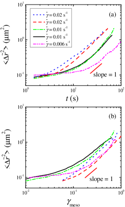
Figure 6: (Color online) (a) The mean square displacement of the non-affine motion $\Delta\tilde{r}$ as a function of the time $t$ since the start of shear. (b) The same data plotted as a function of the accumulated strain $\gamma_{\rm meso}=\int^{t}_{0}\dot{\gamma}_{\rm meso}(t^{\prime})dt^{\prime}$. The five curves represents five data sets with the same volume fraction $\phi=0.51$ but three different shear rates $\bar{\dot{\gamma}}_{\rm meso}$ as indicated in the figure. The total accumulated strain is the final point reached by each curve in panel (b).

To better understand the mean square displacement curves (Fig. 6), we wish to examine the data being averaged to make these curves. We do so by plotting the distributions of displacements $\Delta\tilde{r}$ in Fig. 7. To better compare the shapes of these distributions, we normalize these displacements by the strain and thus plot $P(\Delta s)$ where $\Delta s\equiv\Delta\tilde{r}/(\gamma^{0.5}_{\rm meso})$; this normalization is motivated by the observation that at large $\gamma_{\rm meso}$, we have $\langle\Delta\tilde{r}^{2}\rangle\sim\gamma_{\rm meso}$ (Fig. 6) Maloney and Robbins (2008). Furthermore, we normalize $P(\Delta s)$ so that the integral over all vectors $\Delta\vec{s}$ is equal to 1, similar to Ref. Maloney and Robbins (2008). Figure 7 shows that the distributions corresponding to small strains are much broader than those corresponding to large strains. For the smallest strain, the distribution has a large exponential tail over 3 orders of magnitude. For larger strains ($\gamma_{\rm meso}>0.1$), the curves are no longer exponential and the tails are shorter, indicating fewer extreme events. These curves appear more like Gaussian distributions. At the larger strain values ($\gamma_{\rm meso}>0.1$), the distributions collapse; this is the same strain regime for which the mean square displacement becomes linear with $\gamma_{\rm meso}$ [Fig. 6(b)]. As the Ref. Maloney and Robbins (2008) suggests, the exponential tail for small strains is similar to what has been seen for individual plastic events Tanguy et al. (2006); Lemaître and Caroli (2007), while the distributions for larger strains are consistent with successive temporally uncorrelated plastic events drawn from the exponential distribution. However, it is possible that these events are spatially correlated, which will be seen below.

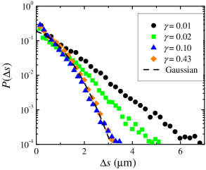
Figure 7: (Color online) Probability distribution function of $\Delta s=\Delta\tilde{r}/\gamma^{0.5}_{\rm meso}$, the nonaffine displacement $\Delta\tilde{r}$ scaled by the local strain $\gamma^{0.5}_{\rm meso}$. The data shown are from one experimental run, using portions of the data corresponding to strain increments $\gamma_{\rm meso}$ = 0.01, 0.02, 0.10, and 0.43. These correspond to time intervals $\Delta t=1.5$, 4.5, 16.5, and 45 s. $P(\Delta s)$ is normalized so that the integral over all vectors $\Delta\vec{s}$ is equal to 1, similar to Ref. Maloney and Robbins (2008). For small strains, the curves have large exponential tails, and for larger strain, the tails become smaller and appear more Gaussian. The dashed line is Gaussian fit for $\gamma_{\rm meso}=0.43$. For this sample, the data and parameters are the same as Fig. 5.

The mean square displacement data we have shown (Fig. 6) treats all three directions equivalently, with the exception that the $x$ displacements have had their nonaffine motions removed. However, the three directions are not equivalent physically: the $x$ direction corresponds to the shear-induced velocity, the $y$ direction is the vorticity direction, and $z$ is the velocity gradient direction. To look for differences in motion between these three directions, we plot the probability distribution of the displacements $[\Delta\tilde{x},\Delta y,\Delta z]$, in Fig. 8. The three distributions agree with each other, and in fact are symmetric around the origin. This suggests that the shear-induced motions are isotropic. Furthermore, they are well-fit by a Gaussian, suggesting that the shear-induced motion liquefies the sample (at least at the large $\gamma_{\rm meso}$ considered for Fig. 8). This seems natural in the context of jamming, where adding more strain moves the sample farther from the jammed state Liu and Nagel (1998). Of course, in our raw data the $\Delta x$ data show a significant bias in the direction of the shear-induced velocity; but it is striking that the non-affine displacements $\Delta\tilde{x}$ show no difference from the displacements in $y$ and $z$, as also found in sheared colloidal glass Besseling et al. (2007); Miyazaki et al. (2004).

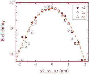
Figure 8: (Color online) Probability distribution functions for non-affine motions in each direction, $\Delta\tilde{x}$ (filled cycle), $\Delta y$ (hollow circle) and $\Delta z$ (hollow triangle). The red curve is a Gaussian fit to the $\Delta\tilde{x}$ data. For this sample, the parameters are the same as Fig. 5 ($\phi=0.51$, $\gamma_{\rm meso}=0.43$, $\bar{\dot{\gamma}}_{\rm meso}=0.0096$ s^-1, $\Delta t=45$ s).

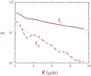
Figure 9: (Color online) Spatial correlation functions $S_{\vec{r}}$ and $S_{\delta r}$ characterizing particle motion. The data are the same as Fig. 5 ($\phi=0.51$, $\gamma_{\rm meso}=0.43$ over 45 s of data, and $\bar{\dot{\gamma}}_{\rm meso}=\gamma_{\rm meso}/\Delta t=0.0096$ s^-1). The solid and dashed lines correspond to $S_{\vec{r}}$ and $S_{\delta r}$ averaged over all the particles in the sample. The dotted lines (red) correspond to exponential fits with length scales $\xi_{\vec{r}}=6.4$ $\mu$m and $\xi_{\delta r}=2.5$ $\mu$m.

Thus far, we have established that shear-induced particle displacements are closely tied to the total applied strain $\gamma_{\rm meso}$ [Fig. 6(b)]. We then introduced the nonaffine motion $\Delta\tilde{r}$ which we find to be isotropic, on the particle scale: individual particles are equally likely to have shear-induced displacements in any direction (Fig. 8). While the distributions of displacements are isotropic, this does not imply that displacements are uncorrelated spatially. To check for this, we calculate two displacement correlation functions as defined in Ref. Weeks et al. (2007); Crocker et al. (2000); Doliwa and Heuer (2000) $:$

$$S_{\vec{r}}(R,\Delta t) = \frac{\langle\Delta\vec{\tilde{r}}_{i}\cdot\Delta\vec{\tilde{r}}_{j}\rangle}{\langle\Delta\tilde{r}^{2}\rangle},$$ (6)

$$S_{\delta r}(R,\Delta t) = \frac{\langle\delta\tilde{r}_{i}\delta\tilde{r}_{j}\rangle}{\langle(\delta\tilde{r})^{2}\rangle},$$ (7)

where the angle brackets indicate an average over all particles; see Refs. Weeks et al. (2007); Doliwa and Heuer (2000) for more details. The mobility is defined as $\delta\tilde{r}=|\Delta\tilde{r}|-\langle|\Delta\tilde{r}|\rangle$, in other words, the deviation of the magnitude of the displacement from the average magnitude of all particle displacements. The correlation functions are computed for the nonaffine displacements, using $\Delta t=45$ s to maximize the “signal” (nonaffine displacements) compared to the “noise” (Brownian motion within cages, on a shorter time scale).

The two correlation functions are shown in Fig. 9 for a representative data set. These functions are large at short separations $R$ and decay for larger $R$, suggesting that neighboring particles are correlated in their motion. In particular, the vector-based correlation $S_{\vec{r}}$ has a large magnitude at small $R$, showing neighboring particles have strongly correlated directions of motion, even given that we are only considering the nonaffine displacements. The two correlation functions decay somewhat exponentially, as indicated by the straight line fits shown in Fig. 9, with decay constants $\xi_{\vec{r}}=6.4$ $\mu$m$=6.1a$ and $\xi_{\delta r}=2.5$ $\mu$m$=2.4a$ (in terms of the particle radius $a$). The larger the slope, the more localized the correlation is. $\xi_{\vec{r}}$ is similar to that found previously for supercooled colloidal liquids, and $\xi_{\delta r}$ is slightly shorter than the prior results Weeks et al. (2007). Overall, these results confirm that the shear-induced particle motion is spatially heterogeneous, quite similar to what has been seen in unsheared dense liquids Ediger et al. (1996); Donati et al. (1998); Weeks et al. (2000, 2007); Kegel and van Blaaderen (2000); Ediger (2000); Doliwa and Heuer (2000) and granular materials Mehta et al. (2008); Goldman and Swinney (2006). The length scale may be equivalent to the correlation length scale for fluidity discussed in Refs. Goyon et al. (2008); Bocquet et al. (2009). For example, an experimental study of sheared polydisperse emulsions found a fluidity length scale comparable to 1-2 droplet diameters near the glass transition Goyon et al. (2008).

Considering all of our data sets, we do not find a strong dependence on either the strain rate $\dot{\gamma}$ or the total strain $\gamma$ for the ranges we consider ($\bar{\dot{\gamma}}_{\rm meso}=0.006-0.02$ s^-1, $\gamma_{\rm meso}=0.3-1.6$). We do not have a large amount of data with which to calculate the correlation functions; unlike prior work, we cannot do a time average Weeks et al. (2007). If we use an exponential function to fit our different data (different strains, strain rates, and volume fractions), the mobility correlation $S_{\delta r}$ yields a length scale $\xi_{\delta r}\approx 1.8-3.9$ $\mu$m and the vector correlation $S_{\vec{r}}$ yields a length scale $\xi_{\vec{r}}\approx 3.2-7.5$ $\mu$m. To check this, we also calculate

$$\xi^{\prime}=\frac{\langle R\cdot S(R)\rangle}{\langle S(R)\rangle}$$ (8)

where the angle brackets indicate averages over $R$; for a perfect exponential, we would have $\xi^{\prime}=\xi$. Using this method, we find more consistent length scales of $\xi^{\prime}_{\delta r}\approx(3.0-4.0)a$ and $\xi^{\prime}_{\vec{r}}\approx(3.5-4.3)a$. Our data do not suggest any dependence of these length scales on the control parameters over the range we investigate. Of course, as $\dot{\gamma}\rightarrow 0$, we would expect to recover the original unstrained sample behavior Yamamoto and Onuki (1997). Similar samples in this volume fraction range were previously found to have length scales with similar values, $\xi_{\delta r}\approx 4a-8a$ and $\xi_{\vec{r}}\approx 6a$ Weeks et al. (2007). However, the time scales for this motion are much longer than that for our sheared samples.

III.3 Defining local plastic deformation

We wish to look for spatially heterogeneous dynamics, that is, how the shear-induced motion takes place locally and how particles cooperate in their motion. Several prior groups have examined local rearrangements in simulations and experiments Falk and Langer (1998); Utter and Behringer (2008); Schall et al. (2007); Goyon et al. (2008), but have used differing ways to quantify the motion. We will discuss those quantities together, and compare them using our data. We have two goals: first, to understand how different measures of local rearrangements reveal different aspects of the motion; and second, to see if the spatial structure of rearranging groups of particles exhibits any particular orientation with respect to the shear direction.

For all of these definitions of rearranging groups of particles, it is useful to define a particle’s nearest neighbors. Our definition of a particle’s nearest neighbors are those particles within the cutoff distance $r_{0}$, set by the first minimum of the pair correlation function $g(r)$.

We start by quantifying the local strain seen by an individual particle, which is based on the average motion of its neighbors. For a particle $i$ with center at $\vec{r}_{i}(t)$, the relative positions of its neighbors $j$ are $\vec{d}_{ij}(t)=\vec{r}_{j}(t)-\vec{r}_{i}(t)$. These neighboring particles move, and their motions over the next interval $\Delta t$ are given by $\Delta\vec{d}_{ij}(t)=\vec{d}_{ij}(t+\Delta t)-\vec{d}_{ij}(t)$, as shown in Fig. 10.

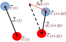
Figure 10: (Color online) Sketch illustrating the definition of the motion of the relative position vector $\Delta\vec{d}_{ij}$ of two neighboring particles, red and blue (dark and light gray). $\vec{r}_{i}(t)$ represents the position of particle $i$ at time $t$, $\vec{d}_{ij}(t)$ is the relative position between particles $i$ and $j$ at time $t$, and $\Delta\vec{d}_{ij}(t)$ is how the vector $\vec{d}_{ij}$ changes over the time interval $(t,t+\Delta t)$.

The strain tensor $\mathbb{E}_{i}$ for this region around particle $i$ is then determined by minimizing the mean squared difference between the actual relative motions $\Delta\vec{d}_{ij}(t)$ and that predicted by $\mathbb{E}_{i}$, in other words, choosing $\mathbb{E}_{i}$ to minimize

$$D^{2}_{i,{\rm min}}={\rm min}\Bigg{[}{\Sigma_{j}}\ \bigg{[}\Delta\vec{d}_{ij}(t)-\mathbb{E}_{i}\vec{d}_{ij}(t)\bigg{]}^{2}\ \Bigg{]}.$$ (9)

The error, $D^{2}_{i,{\rm min}}$, quantifies the plastic deformation of the neighborhood around particle $i$, after removing the averaged linear response $\mathbb{E}_{i}\vec{d}_{ij}(t)$ Falk and Langer (1998). Thus, $D^{2}_{i,{\rm min}}$ is one way to quantify the local nonaffine rearrangement, “local” in the sense of an individual particle $i$ and its neighbors. We term $D^{2}_{i,{\rm min}}$ the “plastic deformation.” Note that the sum is computed over the ten nearest particles $j$ to particle $i$, otherwise the value of $D^{2}_{i,{\rm min}}$ would depend on the number of neighbors. In practice, most of these neighboring particles are within 3.0 $\mu$m of particle $i$, which is comparable to the first minimum of the pair correlation function $g(r)$, which motivates our choice of ten neighbors.

Of course, quite often $\mathbb{E}_{i}$ is different from the overall strain over the imaged volume, which in turn is different from the macroscopically applied strain. In practice, given that the shear is applied in $x$ direction with the velocity gradient along $z$, we only treat the $xz$ components of Eqn. 9; that is, $\vec{d}_{ij}$ and $\mathbb{E}_{ij}$ can be written as $:$

$$\vec{d}_{ij}=\begin{bmatrix}x_{ij}\\ z_{ij}\end{bmatrix},\mathbb{E}_{i}=\begin{bmatrix}\epsilon_{i}^{xx}&\epsilon_{i}^{xz}\\ \epsilon_{i}^{zx}&\epsilon_{i}^{zz}\end{bmatrix}.$$ (10)

To better understand this local strain tensor $\mathbb{E}_{i}$, we follow the method of Ref. Schall et al. (2007); Falk and Langer (1998). If the particle-scale local strain was identical to the imposed strain, we would expect $\epsilon_{i}^{xz}=\gamma_{\rm meso}$ and the other matrix elements to be zero. We find that these expectations are true on average (for example $\langle\epsilon_{i}^{xz}\rangle=\gamma_{\rm meso}$) but that for individual particles their local environment can be quite different. For each experiment, the distributions of all four matrix elements have similar standard deviations, and examining different experiments the standard deviations are between 24% - 39% of $\gamma_{\rm meso}$.

To quantify the measured particle-scale strain, we define the “local strain”

$$\gamma_{i,{\rm micro}}=\epsilon^{xz}_{i}+\epsilon^{zx}_{i}$$ (11)

(using the definition of the strain tensor which is related to $\mathbb{E}$ Landau and Lifshitz (1986)). That is, this quantity is a local approximation to the strain $(\frac{\partial u_{x}}{\partial z}+\frac{\partial u_{z}}{\partial x})$. The local strain $\gamma_{i,{\rm micro}}$ is now a second way to quantify the local rearrangement of the neighborhood around particle $i$, in addition to $D^{2}_{i,{\rm min}}$. The diagonal elements, $\epsilon^{xx}_{i}$ and $\epsilon^{zz}_{i}$, relate to the dilation of the local environment. In particular, the local environment stretches by a factor of $(1+\epsilon^{xx}_{i})$ in the $x$ direction and likewise $(1+\epsilon^{zz}_{i})$ in the $z$ direction. If these matrix elements are zero, then the local environment remains the same; positive matrix elements correspond to expansion and negative matrix elements correspond to contraction. We define the overall dilation as $\delta e_{i}=(1+\epsilon^{xx}_{i})(1+\epsilon^{zz}_{i})-1$, which is a third way to quantify the local rearrangement around particle $i$.

A fourth way to consider local particle motion is the previously defined nonaffine displacement, $\Delta\tilde{r}^{2}$. The key difference is that $D^{2}_{\rm min}$, $\gamma_{\rm micro}$, and $\delta e$ all are derived from the actual particle motion $\Delta r$, whereas $\Delta\tilde{r}^{2}$ removes the motion caused by $\gamma_{\rm meso}$ (through Eqn. 3).

To demonstrate how neighboring particles rearrange and result in larger values of these various parameters, Fig. 11 shows an example using real trajectories. The original positions of the particles are shown, along with displacement vectors indicating where they move after the sample is strained with $\gamma_{\rm meso}=0.58$. The overall strain is seen in that particles near the top move farther than those at the bottom; however, the red (dark) particle in the middle has an unusual motion, moving downward in the $-z$ direction. Figure 11(b) shows the motion of the surrounding particles, as seen in the reference frame attached to the red (dark) particle. It is these displacements that are used in the calculation Eqn. 10. Figure 11(c) shows the predicted final positions of the particles (drawn large) based on $\mathbb{E}_{i}$, as compared to the actual final positions (drawn small); the red (dark) particle is considered “particle $i$”. This local region experiences both shear and a strong dilation in the $z$ direction, both captured by $\mathbb{E}_{i}$. The differences between the predicted and actual final positions result in a moderately large value of $D^{2}_{\rm min}=56$ $\mu$m². In particular, note that $D^{2}_{\rm min}$ is defined based on vectors pointing from the red (dark) reference particle to the other particles, and because the red particle moves downward, the vectors are all greatly stretched and this increases $D^{2}_{\rm min}$. Finally, Fig. 11(d) shows the positions of the same particles after the strain has been applied, where now the box represents the mesoscopic strain $\gamma_{\rm meso}=0.58$. The large spheres represent the expected positions if the motion was affine, and the small spheres show the actual positions. Differences between the expected and actual positions result in large values of the nonaffine displacement $\Delta\tilde{r}$. For the red (dark) particle, $\Delta\tilde{r}=2.97$ $\mu$m. Overall, the anomalous motion of the central particle $i$ is because under the large local strain, this particle makes a large jump out of its original cage. It is these sorts of unusual motions that result in large plastic deformations within the sample.

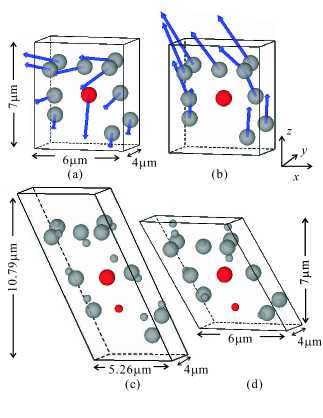
Figure 11: (Color online.) These four sketches show different portrayals of a particle with unusual motion. (a) Particle motion as seen in the laboratory reference frame. The arrows indicate displacement vectors. (b) Similar to (a) except the motion are in the reference frame where the central red (darker) particle is motionless. (c) The large spheres correspond to the expected positions of the particles, and the smaller spheres correspond to the actual positions of the particles. The distortion of the box and the expected positions of the particles are calculated based on the measured local strain tensor $\mathbb{E}_{i}$, where the red (darker) particle is particle $i$. For this local neighborhood, we have $\gamma_{\rm micro}=0.73$ and a dilation primarily in the $z$ direction ($\epsilon^{xx}=-0.1,\epsilon^{zz}=0.5$, and $\delta e=0.35$). (d) The positions of the same particles after the strain has been applied, where now the box represents the mesoscopic strain $\gamma_{\rm meso}=0.58$. The large spheres represent the expected positions if the motion was affine, and the small spheres show the actual positions. For all panels, to show the displacements in three dimensions better, the radii of the large spheres are 0.5 of the real scale. The data correspond to a sample with $\phi=0.51$, $\gamma_{\rm meso}=0.58$, $\bar{\dot{\gamma}}_{\rm meso}=0.014$ s^-1, and $\Delta t=40$ s.

III.4 Collective particle motions

To investigate the relationships between these quantities, a 3 $\mu$m-thin $y$ slice of a sample with volume fraction $\phi=0.51$ is shown in several ways in Fig. 12. In panel (a), the $x$ displacement is shown, making the strain apparent. Panel (b) shows the original Voronoi volumes for each particle at $t=0$. The Voronoi cell for each particle is defined as the volume closer to the center of that particle than to any other particle. In subsequent panels, the darker colors indicate larger local rearrangements, as measured by the non-affine displacement $\Delta\tilde{r}^{2}$ [panel (c)], plastic deformation $D^{2}_{\rm min}$ [panel (d)], local strain $\gamma_{\rm micro}$ [panel (e)], and dilation $\delta e$ [panel (f)]. It can be seen that the darker colored particles cluster together, indicating that for each of these measures of local rearrangement, the motions are spatially heterogeneous Schall et al. (2007). This is a real-space picture showing conceptually what is indicated by the correlation functions in Fig. 9, that neighboring particles have similar motions. These pictures are qualitatively similar to those seen for thermally-induced cage rearrangements in supercooled liquids Kegel and van Blaaderen (2000); Weeks et al. (2000); Donati et al. (1998); Yamamoto and Onuki (1998); Berthier (2004) and glasses Courtland and Weeks (2003); Vollmayr-Lee et al. (2002); Stevenson et al. (2006); Goldman and Swinney (2006); Kawasaki et al. (2007). Furthermore, by comparing these images, it is apparent that particles often have large values of several quantities simultaneously; in particular compare panels (c) and (d), and panels (e) and (f). While the correspondence is not exact, it suggests that all four of these ideas are capturing similar features of rearranging regions. However, it is also clear that there are differences between (c) and (d) as compared to (e) and (f). In the latter two panels, the region of high activity is spread out over a larger area; more of the particles are deforming by these measures at the same time. Nonetheless, in all four cases, the particles around $x\approx 2-4$ $\mu$m are experiencing the most extreme deformations.

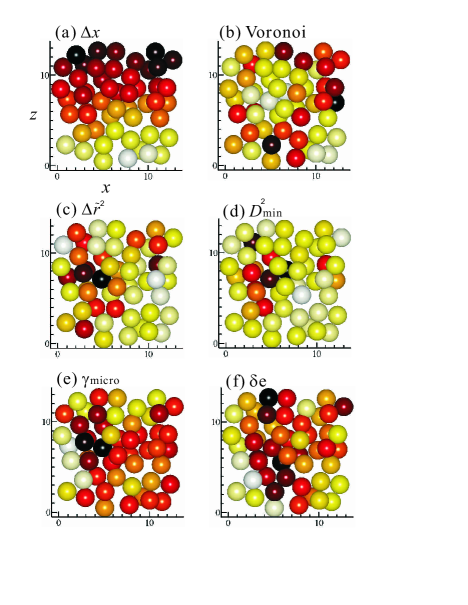
Figure 12: A 3 $\mu$m thin cut through the sample, showing the $xz$ shear plane; the axes are as labeled in (a). The particles are drawn in their location at $t=0$, the start of this strain half-cycle. (a) Darker particles have larger values of $\Delta x$, thus indicating the applied strain. The top particles (large $z$) are moving left (dark colors) and the bottom particles are moving right (light colors). (b) Darker particles have larger Voronoi volumes at $t=0$. (c) Darker particles have larger values of the non-affine motion $\Delta\tilde{r}^{2}$. (d) Darker particles have larger values of the plastic deformation $D^{2}_{\rm min}$. (e) Darker particles have larger values of the local strain $\gamma_{\rm micro}$. (f) Darker particles have larger values of the dilation $\delta e$. The sample is the same as the data shown in Fig. 5; see that figure caption for details.

The Voronoi volume [Fig. 12(b)] has previously been found to be slightly correlated with particle motion in unsheared colloidal supercooled liquids Weeks and Weitz (2002); Conrad et al. (2006); that is, particles with large Voronoi volumes have more space to move and thus are likely to have larger displacements than average. Here it appears that there is no correlation between the Voronoi volume and the particle motion, suggesting that for these strained samples the local volume is not a crucial influence on the motion Miyazaki et al. (2004). This is probably because in the end, all cages must rearrange for the strain to occur.

To demonstrate the relationships between the measures of plastic deformation more quantitatively, we compute 2D histograms comparing pairs of the variables, shown in Fig. 13. The darker color indicates larger joint probability, and the dotted line represents the mean value of the quantity on the vertical axis corresponding to the quantity on the horizontal axis. Figure 13(a) shows that on average, particles with a large plastic deformation $D_{\rm min}^{2}$ are also much likelier to have a large nonaffine displacement $\Delta\tilde{r}^{2}$. This is suggested by the specific example shown in Fig. 11(c,d). Similarly, Fig. 13(b) shows that a particle’s microscopic strain $\gamma_{\rm micro}$ is well correlated with the dilation $\delta e$. For these data, the mesoscopic strain is $\gamma_{\rm meso}=0.43$; particles with $\gamma_{\rm micro}<\gamma_{\rm meso}$ are more often in local environments that contract ($\delta e<0$), and vice-versa. As a contrast, Fig. 13(c) shows a somewhat weaker correlation between $D^{2}_{\rm min}$ and $\gamma_{\rm micro}$. The Pearson correlation coefficients between these quantities are $C(D^{2}_{\rm min},\Delta\tilde{r}^{2})=0.43\pm 0.11$, $C(\gamma_{\rm micro},\delta e)=0.42\pm 0.09$, and $C(\gamma_{\rm micro},D^{2}_{\rm min})=0.17\pm 0.05$. The uncertainties are from the standard deviations of the correlation coefficients from the nine different experiments we conducted.

Overall, Fig. 13 suggests that $D_{\rm min}^{2}$ and $\Delta\tilde{r}^{2}$ both capture the idea of plastic deformation Lemaître and Caroli (2007). The correspondence between these two variables is nontrivial, given that $\Delta\tilde{r}^{2}$ is based on trajectories with the overall strain removed (the strain computed from all observed particles), whereas $D^{2}_{\rm min}$ only accounts for the very localized strain of the neighboring particles. In contrast, $\gamma_{\rm micro}$ and $\delta e$ are well-suited to examine particles moving in atypical ways; typical particles have $\gamma_{\rm micro}\approx\gamma_{\rm meso}$ and $\delta e=0$. These two separate ideas (plastic deformation and atypicality) are only weakly correlated. Other than the three specific comparisons shown in Fig. 13, all other comparisons are even less correlated ($|C|<0.1$). We also examined the quantities $|\gamma_{\rm micro}-\gamma_{\rm meso}|$ and $|\delta e|$ as ways to measure the deviations from typical behavior; these quantities are also only weakly correlated to the other measures of deformation.

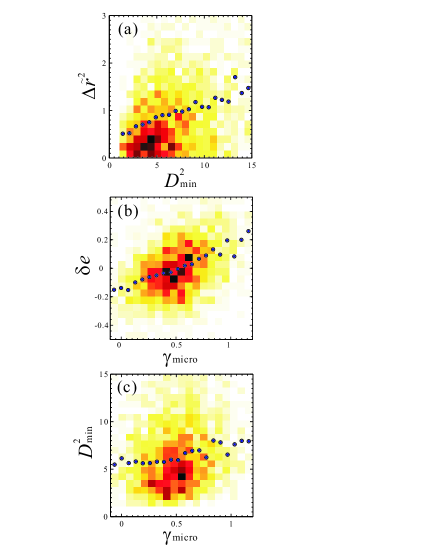
Figure 13: (Color online) 2D histograms of (a) $D^{2}_{\rm min}$ and $\Delta\tilde{r}^{2}$, (b) $\gamma_{\rm micro}$ vs. dilation $\delta e$ and (c) $\gamma_{\rm micro}$ and $D^{2}_{\rm min}$. The sample has the same parameters as Fig. 5; see that caption for details. In these histograms, darker colors stand for the larger probability. The dotted lines are the average values of the $y$ axis corresponding to each value on the $x$ axis. The correlation coefficients between each pair of variables are (a) $C=0.43\pm 0.11$, (b) $C=0.42\pm 0.09$, and (c) $C=0.17\pm 0.05$; see text for details.

We now return to the question of the isotropy of the motion. Figure 8 indicates that the distribution of all particle motions is isotropic, but it is possible that the spatially heterogeneous groups of highly mobile particles shown in Fig. 12 are themselves oriented along a preferred direction. To investigate the 3D structures of these relaxation regions, we quantify the sizes of these active regions in the $x$, $y$ and $z$ directions. To start, we define connected neighboring particles as those with separations less than $r_{0}$, the distance where pair correlation function $g(r)$ reaches its first minimum. (Note that this is slightly different from the neighbor definition used for Eqn. 9; see the discussion following that equation.) For a given quantity, we consider active particles as those in the top 20% of that quantity, similar to prior work Donati et al. (1998); Weeks et al. (2000); Courtland and Weeks (2003); Yamamoto and Onuki (1997). We then define the active region as a cluster of connected active particles. For example, Fig. 14 shows a cluster of particles with large non-affine displacements [panel (a)] and a cluster with large plastic deformations [panel (b)]. Each cluster is drawn from the same data set, and the particles drawn in red (darker) are common to both clusters. (Note that clusters drawn based on $\gamma_{\rm micro}$ and $\delta e$ are smaller. In Fig. 12(e,f), more regions have large values of these parameters, but the top 20% most active are not clustered to the extent they are in Fig. 12(c,d).)

We wish to understand if the shapes of such clusters show a bias along any particular direction. It is important that the experimental observation volume not bias the result, so from within the observed 3D volume we consider only particles that start within an isotropic cube of dimensions 15$\times$15$\times$15 $\mu$m³. The size of this cube is chosen to be the largest cube for which all the particles are within the optical field of view for the full half-cycle of shear for all experiments. (See the related discussion at the end of Sec. II.) Within this isotropic volume, we consider the largest cluster from each experiment and for each considered variable. We then define the extent of that cluster in each direction from the positions of each particle within the cluster as $x_{\rm extent}=\max(x_{i})-\min(x_{i})$ and similarly for $y$ and $z$.

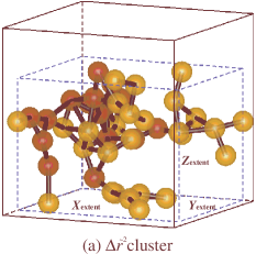
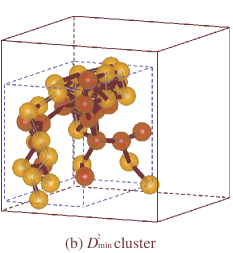
Figure 14: (Color online.) A cluster of neighboring particles with large values of (a) non-affine motion $\Delta\tilde{r}^{2}$ and (b) plastic deformation $D^{2}_{\rm min}$. To avoid biasing the cluster shape, the particles are drawn from within a 15$\times$15$\times$15 $\mu$m³ cube (solid lines). The dashed lines indicate the spatial extent of the two cluster shapes in each direction. The cluster in (a) is $14\times 12\times 11$ $\mu$m³ and the cluster in (b) is $8\times 14\times 10$ $\mu$m³. The red particles are common between the two clusters, and the black bonds indicate neighboring particles; particle sizes are drawn 0.8 times the actual scale, to make the connections more visible. In each case, the particles shown are the top 20% for the parameter chosen. The data corresponds to the same parameters as in Fig. 5; see that caption for details.

Anisotropic cluster shapes would be manifested by systematic differences in the relative magnitudes of $x_{\rm extent}$, $y_{\rm extent}$, and $z_{\rm extent}$. We compare these in Fig. 15 for clusters of particles with large non-affine motion $\Delta\tilde{r}^{2}$ [panel (a)] and large plastic deformation $D^{2}_{\rm min}$ [panel (b)]. The comparison is made by using the ratios $y_{\rm extent}/x_{\rm extent}$ and $z_{\rm extent}/x_{\rm extent}$, thus normalizing the extent in the $y$ and $z$ directions by that of the shear velocity direction $x$. Thus, if a cluster has the same extent in $x$ and $y$, $y_{\rm extent}/x_{\rm extent}$ should be equal to $1$, along the vertical dashed line. Similarly, for the same extent in $x$ and $z$, points should be along the horizontal dashed line with $z_{\rm extent}/x_{\rm extent}=1$. If the extent is the same for $y$ and $z$, the points should be along the diagonal line with $y_{\rm extent}/x_{\rm extent}=z_{\rm extent}/x_{\rm extent}$. For an isotropic cluster with same size in all dimensions, the point should be in the center (1,1).

As shown in Fig. 15, for all of our data, we find no systematic anisotropy; the cluster extent ratios are mostly clustered around the isotropic point (1,1). Due to random fluctuations, no cluster is perfectly isotropic, yet the points seem fairly evenly distributed around the three dashed lines. Thus, while the shear-induced rearrangements take place in localized regions (Fig. 12), the data indicate that these regions on average have no directional bias. This seems true for both the nonaffine displacements $\Delta\tilde{r}^{2}$ in Fig. 15(a) and the plastic deformation $D^{2}_{\rm min}$ in Fig. 15(b).

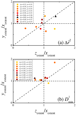
Figure 15: Comparison between the cluster extent in $x$, $y$ and $z$, based on different variables. (a) Particles with the largest non-affine motion $\Delta\tilde{r}$. (b) Particles with the largest plastic deformation $D^{2}_{\rm min}$. The symbols represent different volume fractions: $\phi=0.51$ (circles), 0.56 (triangles) and 0.57 (squares). Colors (or grays from light to dark) represent different accumulative strains $\gamma_{\rm meso}=0.3-0.9$. The clusters are comprised of the top 20% of the particles with the given characteristic.

IV Discussion

We examined the microscopic plastic deformations occurring in several sheared dense colloidal suspensions. Our first main observation is that on average, individual particles have no bias in their direction of motion, other than that trivially imposed by the strain. When this imposed motion is removed from the particle trajectories, the remaining shear-induced motion is isotropic: particles are equally likely to move in any direction. Our second main observation is on the shape of groups of particles undergoing plastic rearrangements. There are several ways to determine which particles are rearranging, and we have shown that all of these are useful for highlighting local regions of deformation. Furthermore, the shapes of these regions are also isotropic. However, we cannot rule out that with more data and subtler analysis, we might find anisotropies in particle motion Furukawa et al. (2009).

In our results, we find little dependence on the overall volume fraction $\phi$, total strain, or strain rate. For the volume fraction, all of our samples are dense liquids with $\phi<\phi_{G}$. At significantly lower volume fractions, presumably particles would not be caged and the shear-induced rearrangements might be quite different Pine et al. (2005). At higher volume fractions $\phi>\phi_{G}$, prior work has seen similar results Besseling et al. (2007); Schall et al. (2007) although not examined the shapes of the rearranging regions in detail. It is possible that results in glassy samples might be different, given that near $\phi_{G}$ slight changes in volume fraction have large consequences Cheng et al. (2002), but we have not seen clear evidence of that in our data. For the total strain, we have not examined a wide range of parameters. In all cases, we are studying sufficiently large enough strains to induce irreversible, plastic rearrangements.For the strain rates, all of our strain rates are fast enough such that the modified Peclet number $Pe^{\star}$ is at least 7, so that thermally induced diffusive motion is less relevant. It is likely that at slower strain rates (lower Peclet numbers), different behavior would be seen Yamamoto and Onuki (1997).

Previous work Ackerson and Pusey (1988); Ackerson (1990); Haw et al. (1998b, a) found that oscillatory shear can induce crystallization of concentrated colloidal suspensions. The ‘induction time’ of this crystallization is strain dependent: a larger strain amplitude results in shorter induction time. In our experiments, we studied only a limited number of oscillations, and our strain amplitude $\sim$1. We did not observe crystallization in any of our experiments. It is likely that were we to continue our observations for much longer times, we could see the onset of shear-induced crystallization, and so we note that our experiments are probably studying a non-equilibrium state. Additionally, Fig. 4 shows that our strain rate takes a while to stabilize after flow reversal, which again suggests that our results are not in steady-state. Thus, it is possible that our primary observation, that the shear-induced particle rearrangements are isotropic in character, is limited only to the transient regime we observe. It is still intriguing that in this regime, particle motion is so isotropic. For example, Fig. 4 shows that the sample takes a while to requilibrate after shear reversal, yet there is no obvious signature of this in the particle motion or the configurations of the particles. Likewise, presumably the long-term crystallization will be caused by anisotropic motion (and result in further anisotropic motion), but no signs of this are present in the early-time amorphous samples we study. It would be interesting to conduct longer-term experiments to relate the particle rearrangements to those resulting in crystallization. Alternatively, it would be also interesting to use a cone-and-plate geometry shear cell capable of indefinitely large strains Besseling et al. (2009), to reach the steady-state constant shear regime.

V Acknowledgments

We thank R. Besseling, J. Clara Rahola, and V. Prasad for helpful discussions. This work was supported by the National Science Foundation (DMR-0603055 and DMR-0804174).

References

- Angell et al. (2000) C. A. Angell, K. L. Ngai, G. B. McKenna, P. F. McMillan, and S. W. Martin, J. Appl. Phys. 88, 3113 (2000).
- Coussot and Gaulard (2005) P. Coussot and F. Gaulard, Phys. Rev. E 72, 031409 (2005).
- Ubbink et al. (2008) J. Ubbink, A. Burbidge, and R. Mezzenga, Soft Matter 4, 1569 (2008).
- Mezzenga et al. (2005) R. Mezzenga, P. Schurtenberger, A. Burbidge, and M. Michel, Nature Mater. 4, 729 (2005).
- Liu and Nagel (1998) A. J. Liu and S. R. Nagel, Nature 396, 21 (1998).
- Coussot et al. (2002) P. Coussot, J. S. Raynaud, F. Bertrand, P. Moucheront, J. P. Guilbaud, H. T. Huynh, S. Jarny, and D. Lesueur, Phys. Rev. Lett. 88, 218301 (2002).
- Huang et al. (2005) N. Huang, G. Ovarlez, F. Bertrand, S. Rodts, P. Coussot, and D. Bonn, Phys. Rev. Lett. 94, 028301 (2005).
- Merkt et al. (2004) F. S. Merkt, R. D. Deegan, D. I. Goldman, E. C. Rericha, and H. L. Swinney, Phys. Rev. Lett. 92, 184501 (2004).
- Spaepen (1977) F. Spaepen, Acta Mater. Acta Metall. 25, 407 (1977).
- Sheng et al. (2007) H. W. Sheng, H. Z. Liu, Y. Q. Cheng, J. Wen, P. L. Lee, W. K. Luo, S. D. Shastri, and E. Ma, Nature Mater. 6, 192 (2007).
- Schuh et al. (2007) C. A. Schuh, T. C. Hufnagel, and U. Ramamurty, Acta Mater. 55, 4067 (2007).
- Pusey and van Megen (1986) P. N. Pusey and W. van Megen, Nature 320, 340 (1986).
- Haw (2002) M. D. Haw, J. Phys.: Cond. Matt. 14, 7769 (2002).
- Suresh (2006) S. Suresh, Nature Mater. 5, 253 (2006).
- Schall et al. (2007) P. Schall, D. A. Weitz, and F. Spaepen, Science 318, 1895 (2007).
- Habdas and Weeks (2002) P. Habdas and E. R. Weeks, Curr. Opin. in Colloid & Interface Science 7, 196 (2002).
- Prasad et al. (2007) V. Prasad, D. Semwogerere, and E. R. Weeks, J. Phys.: Cond. Matt. 19, 113102 (2007).
- Elliot and Poon (2001) M. S. Elliot and W. C. K. Poon, Adv. Colloid Interface Sci. 92, 133 (2001).
- van Megen and Pusey (1991) W. van Megen and P. N. Pusey, Phys. Rev. A 43, 5429 (1991).
- Speedy (1998) R. J. Speedy, Mol. Phys. 95, 169 (1998).
- Brambilla et al. (2009) G. Brambilla, D. E. Masri, M. Pierno, L. Berthier, L. Cipelletti, G. Petekidis, and A. B. Schofield, Phys. Rev. Lett. 102, 085703 (2009).
- O’Hern et al. (2003) C. S. O’Hern, L. E. Silbert, A. J. Liu, and S. R. Nagel, Phys. Rev. E 68, 011306 (2003).
- Bernal (1964) J. D. Bernal, Proc. Roy. Soc. London. Series A 280, 299 (1964).
- Torquato et al. (2000) S. Torquato, T. M. Truskett, and P. G. Debenedetti, Phys. Rev. Lett. 84, 2064 (2000).
- Donev et al. (2004) A. Donev, S. Torquato, F. H. Stillinger, and R. Connelly, Phys. Rev. E 70, 043301 (2004).
- O’Hern et al. (2004) C. S. O’Hern, L. E. Silbert, A. J. Liu, and S. R. Nagel, Phys. Rev. E 70, 043302 (2004).
- van Blaaderen and Wiltzius (1995) A. van Blaaderen and P. Wiltzius, Science 270, 1177 (1995).
- van Megen and Underwood (1993) W. van Megen and S. M. Underwood, Phys. Rev. E 47, 248 (1993).
- van Megen and Underwood (1994) W. van Megen and S. M. Underwood, Phys. Rev. E 49, 4206 (1994).
- Snook et al. (1991) I. Snook, W. van Megen, and P. Pusey, Phys. Rev. A 43, 6900 (1991).
- Bartsch et al. (1993) E. Bartsch, V. Frenz, S. Moller, and H. Sillescu, Physica A 201, 363 (1993).
- Bartsch (1995) E. Bartsch, J. Non-Cryst. Solids 192-193, 384 (1995).
- Mason and Weitz (1995) T. G. Mason and D. A. Weitz, Phys. Rev. Lett. 75, 2770 (1995).
- Falk and Langer (1998) M. L. Falk and J. S. Langer, Phys. Rev. E 57, 7192 (1998).
- Goyon et al. (2008) J. Goyon, A. Colin, G. Ovarlez, A. Ajdari, and L. Bocquet, Nature 454, 84 (2008).
- Bocquet et al. (2009) L. Bocquet, A. Colin, and A. Ajdari, Phys. Rev. Lett. 103, 036001 (2009).
- Yamamoto and Onuki (1997) R. Yamamoto and A. Onuki, Europhys. Lett. 40, 61 (1997).
- Miyazaki et al. (2004) K. Miyazaki, D. R. Reichman, and R. Yamamoto, Phys. Rev. E 70, 011501 (2004).
- Besseling et al. (2007) R. Besseling, E. R. Weeks, A. B. Schofield, and W. C. K. Poon, Phys. Rev. Lett. 99, 028301 (2007).
- Maeda and Takeuchi (1981) K. Maeda and S. Takeuchi, Phil. Mag. A 44, 643 (1981).
- Shi and Falk (2005) Y. Shi and M. L. Falk, Phys. Rev. Lett. 95, 095502 (2005).
- Cheng et al. (2002) Z. Cheng, J. Zhu, P. M. Chaikin, S.-E. Phan, and W. B. Russel, Phys. Rev. E 65, 041405 (2002).
- Weeks et al. (2000) E. R. Weeks, J. C. Crocker, A. C. Levitt, A. Schofield, and D. A. Weitz, Science 287, 627 (2000).
- Wang et al. (2006) Y. Wang, K. Krishan, and M. Dennin, Phys. Rev. E 74, 041405 (2006).
- Utter and Behringer (2008) B. Utter and R. P. Behringer, Phys. Rev. Lett. 100, 208302 (2008).
- Petekidis et al. (2002) G. Petekidis, A. Moussaïd, and P. N. Pusey, Phys. Rev. E 66, 051402 (2002).
- Antl et al. (1986) L. Antl, J. W. Goodwin, R. D. Hill, R. H. Ottewill, S. M. Owens, S. Papworth, and J. A. Waters, Colloid Surf. 17, 67 (1986).
- Dinsmore et al. (2001) A. D. Dinsmore, E. R. Weeks, V. Prasad, A. C. Levitt, and D. A. Weitz, Appl. Opt. 40, 4152 (2001).
- Auer and Frenkel (2001) S. Auer and D. Frenkel, Nature 413, 711 (2001).
- Henderson et al. (1996) S. I. Henderson, T. C. Mortensen, S. M. Underwood, and W. van Megen, Physica A 233, 102 (1996).
- Schöpe et al. (2007) H. J. Schöpe, G. Bryant, and W. van Megen, J. Chem. Phys. 127, 084505 (2007).
- Gasser et al. (2001) U. Gasser, E. R. Weeks, A. Schofield, P. N. Pusey, and D. A. Weitz, Science 292, 258 (2001).
- Hernández-Guzmán and Weeks (2009) J. Hernández-Guzmán and E. R. Weeks, Proc. Natl. Acad. Sci. (2009).
- Haw et al. (1998a) M. D. Haw, W. C. K. Poon, and P. N. Pusey, Phys. Rev. E 57, 6859 (1998a).
- Duff and Lacks (2007) N. Duff and D. J. Lacks, Phys. Rev. E 75, 031501 (2007).
- Dullens et al. (2006) R. P. A. Dullens, D. G. A. L. Aarts, and W. K. Kegel, Phys. Rev. Lett. 97, 228301 (2006).
- ten Wolde et al. (1996) P. R. ten Wolde, M. J. Ruiz-Montero, and D. Frenkel, J. Chem. Phys. 104, 9932 (1996).
- Steinhardt et al. (1983) P. J. Steinhardt, D. R. Nelson, and M. Ronchetti, Phys. Rev. B 28, 784 (1983).
- van Blaaderen et al. (1992) A. van Blaaderen, A. Imhof, W. Hage, and A. Vrij, Langmuir 8, 1514 (1992).
- Shereda et al. (2008) L. T. Shereda, R. G. Larson, and M. J. Solomon, Phys. Rev. Lett. 101, 038301 (2008).
- Crocker and Grier (1996) J. C. Crocker and D. G. Grier, J. Colloid Interface Sci. 179, 298 (1996).
- Besseling et al. (2009) R. Besseling, L. Isa, E. Weeks, and W. Poon, Adv. Colloid Interface Sci. 146, 1 (2009).
- Chan et al. (2004) C.-L. Chan, W.-Y. Woon, and I. Lin, Phys. Rev. Lett. 93, 220602 (2004).
- Lauridsen et al. (2004) J. Lauridsen, G. Chanan, and M. Dennin, Phys. Rev. Lett. 93, 018303 (2004).
- Cohen et al. (2006) I. Cohen, B. Davidovitch, A. B. Schofield, M. P. Brenner, and D. A. Weitz, Phys. Rev. Lett. 97, 215502 (2006).
- Lemaître and Caroli (2007) A. Lemaître and C. Caroli, Phys. Rev. E 76, 036104 (2007).
- Maloney and Robbins (2008) C. E. Maloney and M. O. Robbins, J. Phys.: Cond. Matt. 20, 244128 (2008).
- Weeks and Weitz (2002) E. R. Weeks and D. A. Weitz, Phys. Rev. Lett. 89, 095704 (2002).
- Delogu (2008) F. Delogu, Phys. Rev. Lett. 100, 075901 (2008).
- Pine et al. (2005) D. J. Pine, J. P. Gollub, J. F. Brady, and A. M. Leshansky, Nature 438, 997 (2005).
- Eisenmann et al. (2009) C. Eisenmann, C. Kim, J. Mattsson, and D. A. Weitz, unpublished (2009).
- Tanguy et al. (2006) A. Tanguy, F. Leonforte, and J. L. Barrat, Eur. Phys. J. E 20, 355 (2006).
- Weeks et al. (2007) E. R. Weeks, J. C. Crocker, and D. A. Weitz, J. Phys.: Cond. Matt. 19, 205131 (2007).
- Crocker et al. (2000) J. C. Crocker, M. T. Valentine, E. R. Weeks, T. Gisler, P. D. Kaplan, A. G. Yodh, and D. A. Weitz, Phys. Rev. Lett. 85, 888 (2000).
- Doliwa and Heuer (2000) B. Doliwa and A. Heuer, Phys. Rev. E 61, 6898 (2000).
- Ediger et al. (1996) M. D. Ediger, C. A. Angell, and S. R. Nagel, J. Phys. Chem. 100, 13200 (1996).
- Donati et al. (1998) C. Donati, J. F. Douglas, W. Kob, S. J. Plimpton, P. H. Poole, and S. C. Glotzer, Phys. Rev. Lett. 80, 2338 (1998).
- Kegel and van Blaaderen (2000) W. K. Kegel and A. van Blaaderen, Science 287, 290 (2000).
- Ediger (2000) M. D. Ediger, Annu. Rev. Phys. Chem. 51, 99 (2000).
- Mehta et al. (2008) A. Mehta, G. C. Barker, and J. M. Luck, Proc. Natl. Acad. Sci. 105, 8244 (2008).
- Goldman and Swinney (2006) D. I. Goldman and H. L. Swinney, Phys. Rev. Lett. 96, 145702 (2006).
- Landau and Lifshitz (1986) L. D. Landau and E. M. Lifshitz, Theory of Elasticity, Course of Theoretical Physics (1986), vol. 7, chap. 1, 3rd ed.
- Yamamoto and Onuki (1998) R. Yamamoto and A. Onuki, Phys. Rev. Lett. 81, 4915 (1998).
- Berthier (2004) L. Berthier, Phys. Rev. E 69, 020201 (2004).
- Courtland and Weeks (2003) R. E. Courtland and E. R. Weeks, J. Phys.: Cond. Matt. 15, 359 (2003).
- Vollmayr-Lee et al. (2002) K. Vollmayr-Lee, W. Kob, K. Binder, and A. Zippelius, J. Chem. Phys. 116, 5158 (2002).
- Stevenson et al. (2006) J. D. Stevenson, J. Schmalian, and P. G. Wolynes, Nature Phys. 2, 268 (2006).
- Kawasaki et al. (2007) T. Kawasaki, T. Araki, and H. Tanaka, Phys. Rev. Lett. 99, 215701 (2007).
- Conrad et al. (2006) J. C. Conrad, P. P. Dhillon, E. R. Weeks, D. R. Reichman, and D. A. Weitz, Phys. Rev. Lett. 97, 265701 (2006).
- Furukawa et al. (2009) A. Furukawa, K. Kim, S. Saito, and H. Tanaka, Phys. Rev. Lett. 102, 016001 (2009).
- Ackerson and Pusey (1988) B. J. Ackerson and P. N. Pusey, Phys. Rev. Lett. 61, 1033 (1988).
- Ackerson (1990) B. J. Ackerson, J. Phys.: Cond. Matt. 2, 389 (1990).
- Haw et al. (1998b) M. D. Haw, W. C. K. Poon, P. N. Pusey, P. Hebraud, and F. Lequeux, Phys. Rev. E 58, 4673 (1998b).